The Eigenvalue Analysis of the Density Matrix of 4D Spin Glasses Supports Replica Symmetry Breaking

Abstract

We present a general and powerful numerical method useful to study the density matrix of spin models. We apply the method to finite dimensional spin glasses, and we analyze in detail the four dimensional Edwards-Anderson model with Gaussian quenched random couplings. Our results clearly support the existence of replica symmetry breaking in the thermodynamical limit.

I Introduction

Replica Symmetry Breaking (RSB) MPV was introduced more than twenty years ago PARISI as a crucial tool to describe the low temperature phase of spin glasses SPINGLASSES . One can see replicas as an extension of Statistical Mechanics that can be very useful when studying complex systems, such as structural glasses VETRI or spin glasses SPINGLASSES , where the ergodicity breaking in the low temperature phase cannot be described with the help of an infinitesimal external constant magnetic field.

If on one side there is little doubt MATHEMATICS left about the correctness of the RSB description of the low temperature phase of the mean field models, on the other side the controversy CONTROVERSIAL ; CONTRO-MATH ; JSTATPHYS ; GROUNDSTATES regarding its applicability to finite dimensional systems such as realistic, physical spin glasses, is alive and in good health.

Unfortunately, we are only starting to guess how to address the question of the existence of RSB in real spin glasses from a truly experimental point of view FDT : because of that, and because of the inherent very high complexity of the relevant analytic computations, most of the recent progresses are coming from numerical simulations.

The output data of numerical simulations are never as reliable as analytic (and, even better, rigorous) results. So if on one side the results of numerical simulations of four dimensional spin glasses Zullo ; JSTATPHYS support the RSB scenario (as indeed happens for the three dimensional model JSTATPHYS ) on the other side one can argue that these indications could turn out to be fallacious on larger lattices, on longer time scales, at lower temperatures… (see for example PROBLEMSIMULATIONS, for a typical criticism to typical numerical simulations).

It is clear that new approaches to this important issue are precious: Sinova, Canright, Castillo and MacDonald SINOVA3 have recently proposed such a new tool, that can allow a better study of spin glasses. They have noticed that the spin-spin correlation matrix $\langle\sigma_{i}\sigma_{j}\rangle$ (that we will discuss in better detail in the next section) shares the main properties of a quantum mechanical density matrix YANG : it enjoys positivity, hermiticity and has unit trace (notice that our normalization differs from theirs, see next section). In the low temperature phase the time reversal symmetry is broken, and thus one should expect at least one non vanishing eigenvalue of the density matrix in the thermodynamical limit, due to the extended character of the eigenvector related with the symmetry breaking YANG . What is new is the claim SINOVA3 that the presence of RSB is equivalent to the existence of more than one non vanishing eigenvalues in the thermodynamic limit. Thus armed the authors of SINOVA3, undertook the study of the Edwards-Anderson model with Gaussian couplings in four dimensions, were they found results that they judged inconsistent with the detection of RSB on lattices of linear size up to $6$ (i.e. of volume up to $6^{4}$).

The efforts of SINOVA3, were limited to such small lattice sizes, because the memory and the numerical effort required in their approach grows as $L^{2D}$ (in the following $L$ will be the lattice linear dimension, and $D$ the space dimensionality). It is clear that their simulation strategy and data analysis can sometimes go wrong, as it is evidenced by its failure SINOVA4 in the analysis of the Random Field Ising model. In that case, only turning to the standard numerical strategy JSTATPHYS , that focuses on the Parisi order parameter function, $P(q)$, they could establish SINOVA4 the (plausible) absence of RSB in this model.

Here we present a numerical strategy for the study of the density matrix of spin glass with a cost of the order $L^{D}$. We propose a more convenient data analysis, given the expected behavior of the density of eigenvalues of the density matrix in the thermodynamic limit (see next section and reference CORREALE, ). In this way we have been able to study the Edwards-Anderson model with Gaussian couplings on lattices of volume up to $8^{4}$, at the same temperatures as in SINOVA3, . We obtain results that support an RSB scenario JSTATPHYS . Very interesting information about the density matrix in a RSB scenario can also be obtained through mean field calculations CORREALE . Moreover the numerical approach that we have developed here can be applied to any spin model.

When completing this manuscript, a note reporting another efficient approach to the density matrix spectral problem has appeared HUKUSHIMA . In this work Hukushima and Iba deal with the four dimensional spin glass model with binary (rather than Gaussian like in our case) couplings. They have been able to study lattices of volume $10^{4}$, reaching the same conclusion that we present here, i.e. arguing for the presence of RSB in the infinite volume limit (they also discuss an interesting method for studying temperature chaos).

The layout of the rest of this paper is as follows. In section II we define the model and the associated density matrix, discussing its basic properties and the numerical approach of SINOVA3, . Our own strategy is presented in subsection II.1, and a working example is analyzed in subsection II.2, where the (replica symmetric) ferromagnetic Ising model in four dimensions is analyzed. Our numerical simulations of the Edwards-Anderson model in 4 dimensions are described in section III. Our results are presented and discussed in section IV. Finally, we present our conclusions in section V.

II The Model and its Density Matrix

We consider the four dimensional Edwards-Anderson spin glass in a periodic box of side $L$. The $N$ elementary spins can take binary values, $\sigma_{i}=\pm 1$, and they are defined on the vertices of a single hyper-cubic lattice of size $V=L^{D}$. We consider a first neighbor interaction:

$$H=-\sum_{\langle i,j\rangle}\,\sigma_{i}J_{i,j}\,\sigma_{j}\,.$$ (1)

The quenched couplings, $J_{i,j}=J_{j,i}$, are drawn from a symmetric probability distribution function of zero average and variance $J^{2}$. It is customary to take $J$ as unit of temperature, and then to set $J=1$: this is what we do. Two popular choices are the one of a binary probability distribution $J_{i,j}=\pm 1$ or to take $J$ Gaussian distributed. Here, we draw the quenched random couplings from a Gaussian distribution (also in order to allow a direct comparison with the work of SINOVA3, ). For all the relevant observables one first compute the thermal average on a single realization of the couplings (sample), hereafter denoted by $\langle\ldots\rangle$, and later the average with respect to the couplings is performed (we denote this disorder average by an over-line). The model (1) undergoes a spin glass transition SG4D-GAUSS at $T_{\mathrm{c}}=1.80\pm 0.01$.

The average over the couplings $J_{i,j}$ induces a (trivial) gauge invariance GAUGE-SG in the model. If one chooses a generic binary value for each lattice site, $\eta_{i}=\pm 1$, disorder averaged quantities are invariant under the transformation

$$J_{i,j} \longrightarrow \eta_{i}J_{i,j}\eta_{j}\,,$$ (2)

$$\sigma_{i} \longrightarrow \eta_{i}\sigma_{i}\,.$$ (3)

Now let $\eta_{i}$ be a random number that takes the probability $\frac{1}{2}$ the values $\pm 1$. If one considers the spin-spin correlation function, the symmetry (3) yields the disappointing result that

$$\overline{\langle\sigma_{i}\sigma_{j}\rangle}=\eta_{i}\eta_{j}\overline{\langle\sigma_{i}\sigma_{j}\rangle}=\delta_{i,j}\,,$$ (4)

(that is true since this relation is valid for every value of $\eta$) explaining why nobody before references SINOVA3, paid much attention to this quantity. Reference SINOVA3, wisely suggested to look at the correlation function of a single sample as a matrix, $c_{i,j}$. We define here $c_{i,j}$ as

$$c_{i,j}\equiv\frac{1}{L^{D}}\,\langle\sigma_{i}\sigma_{j}\rangle$$ (5)

(notice the difference in the factor $L^{-D}$ with the definition of references SINOVA3, ; SINOVA4, ). The gauge transformation (3) acts on the matrix $c_{i,j}$ as an unitary transformation. Therefore, contrary to the individual elements of $c_{i,j}$ itself, the spectrum of $c_{i,j}$ does not become trivial after the disorder average. It is easy to check SINOVA3 that $c_{i,j}$ is symmetric, positive definite, and has trace equal to one, just like a quantum mechanical density matrix. Thus the corresponding eigenvalues, $1\geq\lambda_{1}\geq\lambda_{2}\geq\ldots\lambda_{N}\geq 0,$ verify

$$1 = \sum_{k=1}^{N}\,\lambda_{k}\,.$$ (6)

Following YANG, the authors of SINOVA3, have argued that in the paramagnetic phase all the $\lambda_{k}$ are of order $\frac{1}{N}$, and thus vanish in the thermodynamical limit. On the other hand in the spin glass phase time reversal symmetry is broken, which implies some non local ordering pattern for the spins (unfortunately only known by the spins themselves), and hence at least one eigenvalue, $\lambda_{1}$ should remain of order one when $N\to\infty$. They also claimed that presence of RSB is equivalent to more than one eigenvalue being of order ${\cal O}(N^{0})$ when $N\to\infty$. Furthermore they stated that each non vanishing eigenvalue corresponds to a pair of pure states: the correspondence to a pair of pure states is because of the global $\sigma\longrightarrow-\sigma$ symmetry of the Hamiltonian (1) and of the matrix $c_{i,j}$. Notice that this might be a clue for the solution of the formidable problem of defining pure states in a finite volume system CONTRO-MATH ; JSTATPHYS . The fact that the presence of more than one extensive eigenvalue (of order ${\cal O}(N^{0})$) when $N\to\infty$ is equivalent to RSB is true in the mean field picture, as can be verified in a mean field analytic computation at the first step of RSB CORREALE .

Combining perturbation theory and droplets ideas it was also possible to tell SINOVA3 that in a non RSB scenario the second eigenvalue should not decay slower than

$$\lambda_{2}\sim L^{-\theta}\,,$$ (7)

where the droplet exponent in four dimensions is THETAEXPONENT $\theta=0.6$–$0.8$. Actually when the lattice size is larger than the correlation length (which might not be the case in the achievable numerical simulations PROBLEMSIMULATIONS ), they expect a much faster decay.

Using the parallel tempering optimized Monte Carlo scheme TEMPERING , the authors of SINOVA3, calculated the matrix $c_{i,j}$, (a computational task of the order $L^{2D}$, since the lack of translational invariance prevents the use of the Fast Fourier transform). They eventually diagonalized the matrix. When comparing results for different disorder realizations, they found very broad distributions of each $\lambda_{k}$, that they tried to characterize by their mean and typical value. They found that the mean and the typical value of the second eigenvalue were decreasing as a function of lattice size in a double logarithmic plot for lattices up to $6^{4}$ (see figure 7 of the second of references SINOVA3, ). Because of that they argued about the absence of RSB in the model.

II.1 An Effective Approach to the Study of the Density Matrix

Studying the spin-spin correlation function $c_{i,j}$ by analyzing the usual density of states $g_{u}$

$$g_{u}(\lambda)=\frac{1}{N}\overline{\sum_{k=1}^{N}\delta(\lambda-\lambda_{k})}$$ (8)

would not work: because of the constraint (6) in the $N\to\infty$ limit $g_{u}(\lambda)$ is a normalized distribution function with support in the $[0,1]$ interval with mean value $0$. In other words, this definition implies that in presence of a generic finite number of extensive eigenvalues for large volumes $g_{u}(\lambda)=\delta(\lambda)$, which does not contain much information.

In our case we cannot weight all the eigenvalues with the same weight: to consider a sensible indicator we can decide to use as weight $\lambda_{k}$ itself, and to define the modified density of states of the matrix $c_{i,j}$:

$$g(\lambda)=\overline{\sum_{k=1}^{N}\lambda_{k}\,\delta(\lambda-\lambda_{k})}\,.$$ (9)

It is natural to expect $g(\lambda)$ to converge in the $N\to\infty$ limit to a function containing a continuous part, plus a delta function at $\lambda=0$ (because a number of order ${\cal O}(N)$ of eigenvalues will be of order ${\cal O}(N^{-1})$). A calculation at one step of RSB CORREALE tells us that this is indeed the case. Moreover in the one step calculation the continuous part do not show any gap, and it covers all the interval between $\lambda=0$ and $\lambda=q_{\mathrm{EA}}$, the Edwards-Anderson order parameter (see also figure 1 of the second of reference SINOVA3, ). Therefore, from the point of view of checking Replica Symmetry Breaking, to concentrate on the behavior of individual eigenvalues does not look the best strategy. Instead, as it is customary when analyzing density of states ORTHOGONAL , one can start by considering the moments for a single disorder realization, $g_{J}(\lambda)$:

$$\int_{0}^{1}\,d\lambda\,\lambda^{r}g_{J}(\lambda)=\sum_{k=1}^{N}\lambda_{k}^{r+1}=\mathrm{Tr}\,c^{r+1}\,.~{}$$ (10)

Our main observation is that we can compute the trace of the $r$-th power of the matrix $c$, using $r$ real replicas (independent systems, with the same realizations of quenched random couplings $J_{i,j}$). Let us define the overlap between replicas $a_{l}$ and $a_{j}$:

$$q^{a_{l},a_{j}}\equiv\frac{1}{N}\,\sum_{i=1}^{N}\,\sigma_{i}^{(a_{l})}\sigma_{i}^{(a_{l})}\,.$$ (11)

Then it is easy to show that

$$\mathrm{Tr}\,c^{r}=\langle q^{a_{1},a_{2}}q^{a_{2},a_{3}}\ldots q^{a_{r},a_{1}}\rangle\,.$$ (12)

Thus, for instance, the (disconnected) spin glass susceptibility is $\chi_{\mathrm{SG}}=N\ \mathrm{Tr}\,c^{2}$. In this language the relationship between non vanishing eigenvalues and the phase transition from the paramagnetic to the spin glass phase is very direct.

It is now very easy to suggest a numerical strategy of order $L^{D}$: make the Monte Carlo simulation in parallel for a discrete number of replicas, and use them to calculate the appropriate number of moments of $g_{J}(\lambda)$. Then use this information to extract the largest eigenvalues of the matrix $c$. Unfortunately standard methods for extracting the probability density from its moments ORTHOGONAL use orthogonal polynomials. Clearly, given the limited numerical accuracy that we can expect to obtain for the $\mathrm{Tr}\,c^{r}$, the use of orthogonality methods is out of the question. We have instead used a cruder method. We define a cost function

$${\cal F}(\xi_{1},\ldots,\xi_{r})=\sum_{l=1}^{r}\,\left(1\ -\ \frac{\sum_{k=1}^{r}\,\xi_{k}^{l}}{\mathrm{Tr}\,c^{l}}\right)^{2}\,,$$ (13)

and minimize it, using the values of the $\xi_{k}$ at the minimum as an approximation to the eigenvalues. This method can be checked on small lattices, using the direct computation of $c$ and its eigenvalues. It turns out (see subsection II.2 and section IV) that it is extremely precise for the first eigenvalue, $\lambda_{1}$, but that already for the second eigenvalue, $\lambda_{2}$ the systematic error is at the $10\%$ level using $12$ replicas. Fortunately we can do better than setting $\lambda_{2}\approx\xi_{2}$. Let us define a (further) modified density of states in which we do not include the first eigenvalue

$$\tilde{g}(\lambda)=\overline{\sum_{k=2}^{N}\lambda_{k}\,\delta(\lambda-\lambda_{k})}\,.$$ (14)

Its moments are

$$\int_{0}^{1}\,d\lambda\,\lambda^{r}\tilde{g}(\lambda)=\overline{\left[\mathrm{Tr}\,c^{r+1}-\lambda_{1}^{r+1}\right]}\equiv\overline{\Delta_{r+1}}\,,~{}$$ (15)

where we have denoted by $\Delta_{r}$ the subtracted traces. The right hand side of equation (15) can be accurately calculated using the cost function, and contains all the information that we need.

One could still worry about the bias induced by our use of the cost function to obtain $\lambda_{1}$. This can be easily controlled, because, since the eigenvalues of the matrix decrease fast with $k$ it turns out that we are always in a situation where we can expect that $\overline{\Delta_{r}}$ is clearly and substantially larger than $\overline{\Delta_{r+1}}$. On the other hand, if the bias on $\lambda_{1}$ is $\delta$, it will affect $\overline{\Delta_{r}}$ of a quantity of the order of $(\delta\ r\ \lambda_{1}^{r-1})$. Therefore, a bias dominated subtracted trace will be characterized by successive moments of $\tilde{g}(\lambda)$ being very similar (see subsection II.2).

Let us conclude this subsection by discussing the different scenarios that could describe the scaling of the subtracted traces, in the $L\to\infty$ limit. For a standard replica symmetric model, such as the usual ferromagnetic Ising model, we expect $\overline{\Delta_{r+1}}={\cal O}(L^{-rD})\,$. In a RSB scenario we expect that for $L\to\infty$ $\overline{\Delta_{r+1}}$ tends to a finite value (and that finite volume corrections due to the eigenvalues that create the $\delta(\lambda)$ in $g(\lambda)$ are of the form ${\cal O}(L^{-rD})$, while iother finite size corrections due to critical fluctuations may not decay so fast). Finally, in a droplet scenario, if one assumes that the subtracted traces are controlled by $\lambda_{2}$, then equation (7) implies that

$$\overline{\Delta_{r}}={\cal O}(L^{-r\theta})\,,$$ (16)

with $\theta=0.6$–$0.8$ in four dimensions (recall that this is an upper bound in the decay of $\lambda_{2}$). The only way out from this scaling behavior in a droplet picture would be to assume that a number of the order $L^{\xi}$ ($\xi>0$) of eigenvalues is of order $L^{-\theta}$: we are not aware of any argument SINOVA3 that would imply the existence of a divergent number of critical eigenvalues in a droplet picture.

II.2 A Simple Example: the Ferromagnetic Ising Model

As a first check we have studied the ferromagnetic Ising model in four dimensions. Here the Hamiltonian has the same form than in (1), but with $J_{i,j}=1$. We have studied the system at $T=0.5T_{\mathrm{c}}$, to prove the deep broken phase with small correlation length (the critical temperature is here ISING4D $T_{\mathrm{c}}=6.68025\pm 0.00004)$). We have simulated in parallel (in this case without parallel tempering, but with an usual heat-bath updating scheme) twelve replicas of lattices of linear size $L=3,4,6$ and $8$, for $3\times 10^{5}$ Monte Carlo steps, starting from a fully ordered state.

In this simple case the density matrix $c_{i,j}$ can be very easily diagonalized. The correlation function $\langle\sigma_{i}\sigma_{j}\rangle$ depends only on the distance between the two spins, $\vec{x}_{i}-\vec{x}_{j}$, and thus the eigenvectors are proportional to $\mathrm{exp}[\mathrm{i}\vec{k}\cdot\vec{x}_{i}]$, where the wave-vectors $\vec{k}$ verify the usual quantization rules on a periodic box. It is straightforward to show that the corresponding eigenvalues are

$$\lambda_{\vec{k}}=\left\langle\,\left|\sum_{i=1}^{N}\,\frac{\mathrm{e}^{\mathrm{i}\vec{k}\cdot\vec{x}_{i}}\sigma_{i}}{L^{D}}\,\right|^{2}\,\right\rangle\,,$$ (17)

and, given the ferromagnetic character of the interaction, the largest eigenvalue corresponds to $\vec{k}=0$ (the magnetization, $M$):

$$\lambda_{1}=\langle M^{2}\rangle\,.$$ (18)

Figure 1: Cost function (13) estimate of the largest eigenvalue of the density matrix, as a function of the number of calculated moments (see equation (15)), for the four dimensional Ising model at $T=0.5T_{\mathrm{c}}$, in a $L=4$ lattice. The horizontal lines correspond to $\langle M^{2}\rangle$ plus or minus one standard deviation.

Figure 2: As in figure 1 but for a $L=8$ lattice.

In figures 1 and 2 we compare our estimate of $\lambda_{1}$ for the $L=4$ and $L=8$ lattices, as obtained from the magnetization (the horizontal band is $\langle M^{2}\rangle$ plus/minus an standard deviation), and from the cost function (13). As both figures show, 12 replicas are surely enough to obtain agreement within errors, which in this case are particularly small.

Figure 3: The subtracted trace, $\Delta_{2}$, as a function of the lattice size, for the four dimensional ferromagnetic Ising model.

Figure 4: As in figure 3 but for $\Delta_{3}$.

Having gained confidence in our procedure we can now check evolution of the subtracted traces with increasing lattice size (figures 3 and 4). The two values are very small, decreasing with the lattice size and almost (but not completely) compatible with zero. One should notice that $\Delta_{3}$ and $\Delta_{2}$ are compatibles within errors for all lattice sizes (we will see in section IV that in the spin glass case the situation is very different): in the ferromagnetic case the real $\Delta_{3}$ and $\Delta_{2}$ are so small that they are completely dominated by the bias discussed in the previous subsection. One might ask how come that we were able to resolve such an small bias, given the comparatively large errors reported in figures 1 and 2: this is due to the strong statistical correlations between$\mathrm{Tr}(c^{r})$ and our estimate for $\lambda_{1}^{r}$.

III The Monte Carlo Simulation

We have studied by numerical simulations the four dimensional Edwards-Anderson spin glass with quenched random Gaussian couplings (1). We have simulated $12$ real replicas in parallel using a heath bath algorithm and Parallel Tempering TEMPERING , on lattices of volume $3^{4}$, $4^{4}$, $6^{4}$ and $8^{4}$. The ratio between full lattice heat bath sweeps and parallel tempering temperature swap attempt was one to one. For all lattice sizes the largest temperature was $T_{\mathrm{max}}=2.7$ and the lowest temperature $T_{\mathrm{min}}=0.8$ (see table 1 for details of the numerical simulation). The probability of accepting a temperature swap was kept at the $60\%$ level. For each replica we have measured the permanence histogram at each temperature, and we checked its flatness. We controlled thermalization by checking that there was no residual temporal evolution in the Binder cumulant and in $\mathrm{Tr}\,c^{12}$.

The main scope of the simulation has been to obtain $\mathrm{Tr}c^{r}$, for $r=2,\ldots,12$, using equation (11). There is an awfully large number of equivalent ways of forming the trace $q^{a_{1},a_{2}}q^{a_{2},a_{3}}\ldots q^{a_{r},a_{1}}$ when one may choose the replica labels $a_{i}$ out of twelve possible values. One needs to find a compromise between loosing statistics and wasting too much time in a given disorder realization (the disorder average is the critical factor controlling statistical error). Our compromise has been the following: given the special importance of this observable JSTATPHYS we have calculated the $\frac{12(12-1)}{2}$ possible overlaps $q^{a_{1},a_{2}}$, and we have computed $\mathrm{Tr}(c^{2})$ using all the $66$ quantities. For traces of higher order we have considered only twelve contributions of the form $q^{i,i+1}q^{i+1,i+2}\ldots q^{i+r,i}$, for $i=1,2,\ldots,12$ (the sums are understood modulo 12).

Figure 5: The Binder cumulant as a function of temperature, for the 4D Edwards-Anderson model on lattices of linear size $L=3$, $4$, $6$ and $8$.

In addition to the $\mathrm{Tr}(c^{r})$ we have measured the Binder cumulant (see figure 5) We have also measured a second adimensional operator

$$B_{3}=\frac{\overline{\mathrm{Tr}\,c^{3}}}{\overline{\mathrm{Tr}\,c^{2}}^{\frac{3}{2}}}\,,$$ (19)

that we show in figure 6.

Figure 6: As in figure 5, but for the $B_{3}$ cumulant.

The theory of finite size scaling FSS predicts that adimensional quantities close to criticality are functions of $L^{1/\nu}(T-T_{\mathrm{c}})$, where $\nu$ is the thermal critical exponent (in $D=4$ one finds Zullo $\nu=1.0\pm 0.01)$). The crossing points signals the spin glass transition at $T_{\mathrm{c}}=1.8$ with similar accuracy for both the cumulants that we have considered. At the lowest temperature that we have reached the $L=6$ and $L=8$ lattices seem to be far enough from the critical region.

$L$	$N_{\mathrm{samples}}$	$N_{\mathrm{measures}}$	$N_{\mathrm{thermal}}$	$N_{\beta}$
3	2800	50000	50000	20
4	2800	50000	50000	20
6	1208	150000	150000	40
8	362	100000	200000	40

Table 1: Relevant parameters of the Monte Carlo simulation. $L$ is the lattice size. $N_{\mathrm{samples}}$ denotes the number of realizations of the Gaussian couplings. The number of Monte Carlo steps (heat bath sweep plus temperature swap attempt) discarded for thermalization was $N_{\mathrm{thermal}}$. $N_{\beta}$ is the number of temperatures simulated in the parallel tempering. Finally, measures were taken during $N_{\mathrm{measures}}$ Monte Carlo steps.

IV Numerical Results

Figure 7: Disorder averaged cost function (13) estimate of the largest eigenvalue of the density matrix, as a function of the number of calculated moments (see equation (15)), for the four dimensional Edwards-Anderson spin glass at $T=1.0$, on a $L=4$ lattice. The horizontal lines correspond to a numerical diagonalization of the matrix $c_{i,j}$ plus or minus a standard deviation.

Figure 8: Disorder averaged $\Delta_{2}$ for the four dimensional Edwards-Anderson spin glass at $T=1.0$ as a function of the number of computed moments, on different lattice sizes.

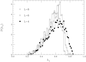
Figure 9: Probability distribution of the largest eigenvalue as calculated in the four dimensional Edwards-Anderson spin glass at $T=1.0$, for lattices of linear size $L=4$, $6$ and $8$. The binning in the $L=8$ lattice was reduced by a factor of two, due to the smaller number of samples.

To compare our results with the ones of SINOVA3, we will specialize here to $T=1.0$. We start by checking on small lattice sizes (see in figure 7 the $L=4$ data) the cost function procedure. In this case the estimate of $\lambda_{1}$ that one can obtain by using the cost function can be compared directly with the result obtained by diagonalization of $c$: we find a fair agreement. For larger lattices we can only check the convergence of $\overline{\Delta_{r}}$ as a function of the number of moments (see figure 8). Again, the convergence looks fast enough for our purposes. We show in figure 9 the probability distribution of $\lambda_{1}$ . The low eigenvalues tail is basically lattice size independent.

Figure 10: Disorder averaged subtracted trace $\overline{\Delta_{2}}$ for the four dimensional Edwards-Anderson spin glass at temperature $T=1.0$ as a function of the lattice size.

Figure 11: As in figure 10 but for $\overline{\Delta_{3}}$.

We show our results for $\overline{\Delta_{2}}$ and $\overline{\Delta_{3}}$ in figure 10 and figure 11, respectively. $\overline{\Delta_{2}}$ is a factor of 10 larger than $\overline{\Delta_{3}}$: our data are not bias dominated (see subsections II.1 and II.2). The fact that the data point for $\overline{\Delta_{3}}$ in the $L=8$ lattice is above the $L=6$ one and at two standard fluctuations from compatibility may be due either to a strong fluctuation, or to a first glimpse of bias effects. If one sticks to the bias hypothesis, the effect on $\overline{\Delta_{2}}$ can be (very conservatively) estimated as the difference of the $L=6$ and $L=8$ data points corresponding to $\overline{\Delta_{3}}$. This difference is well covered by the error in the $L=8$ data point for $\overline{\Delta_{2}}$.

Figure 12: Disorder averaged $\overline{\Delta_{2}}$ as a function of $L^{-D}$ for the four dimensional Edwards-Anderson spin glass at $T=1.0$. The dashed line is for a linear best fit, excluding the $L=3$ data.

Figure 13: Disorder averaged $\overline{\Delta_{2}}$, as a function of $L^{-2\theta}$ for the four dimensional Edwards-Anderson spin glass at $T=1.0$. The droplet $\theta$ exponent is chosen at its lower bound, $\theta=0.6$. The dashed (dotted) line is for a linear best fit, excluding (including) the $L=3$ data point.

After the above considerations we can now proceed to the infinite volume extrapolation. In figure 12 we plot the data for $\overline{\Delta_{2}}$ as a function of $L^{-D}$. It is evident that, letting aside the $L=3$ data, a linear fit is appropriate. The extrapolation to infinite $L$ is definitely different from zero:

$$L\geq 3,\ \overline{\Delta_{2}}=0.0119\pm 0.0003 \chi^{2}/{\mathrm{dof}}=17.8\,,$$ , (20)

$$L\geq 4,\ \overline{\Delta_{2}}=0.0102\pm 0.0004 \chi^{2}/{\mathrm{dof}}=1.73\,.$$ , (21)

In figure 13 we plot the data as they should scale according to the droplet model. A fit to behavior implied by equation (16) yields a very high value of $\chi^{2}/\mathrm{dof}$ either when we include the $L=3$ data or when we exclude them (we use $\theta=0.6$, the lowest possible value THETAEXPONENT ):

$$L\geq 3 \chi^{2}/{\mathrm{dof}}=17\,,$$ , (22)

$$L\geq 4 \chi^{2}/{\mathrm{dof}}=14\,.$$ , (23)

V Conclusions

We have proposed and used a new numerical approach to the study of the density matrix in spin glasses. The original idea of SINOVA3, , namely to introduce the density matrix in the spin glasses context, allows to make interesting calculations CORREALE , and might even prove useful to the definition of pure states in finite volume JSTATPHYS ; CONTRO-MATH .

Our method is a further step beyond the useful approach of of SINOVA3, . The technology we have developed can be safely applied to the study of different spin models. The main limitation of our approach is not related with the use of the density matrix, but with the extreme difficulty in thermalizing large lattices deep in the spin glass phase. Should an efficient Monte Carlo algorithm be discovered, our method would be immediately available, because the computational burden grows only as $L^{D}$. Very recently, another optimized method has been proposed by Hukushima and Iba HUKUSHIMA . Using their method they were able to study $10^{4}$ lattices, using binary rather than Gaussian couplings (which strongly speeds up the simulation).

Using our approach we have been able to show that the density matrix approach for the four dimensional Edwards Anderson model with Gaussian couplings in lattices up to $L=8$, and temperatures down to $T=1.0$ ($\sim 0.56T_{\mathrm{c}}$), is fully consistent with an RSB picture, and that there are serious difficulties with the scaling laws predicted by the alternative droplet model. In this respect, the results are in full agreement with the availables studies JSTATPHYS of the Parisi order parameter, and with the recent results of HUKUSHIMA, . A word of caution is in order: the (postulated) impossibility of getting thermodynamic data in the reachable lattices sizes PROBLEMSIMULATIONS , affects equally to the $P(q)$ approach and to the density matrix approach. However our data for adimensional quantities, such as the Binder or $B_{3}$ cumulant, seem very hard to reconcile with the possibility of a purely finite volume effect.

References

- (1) M. Mézard, G. Parisi and M. A. Virasoro, Spin Glass Theory and Beyond (World Scientific, Singapore 1987).
- (2) G. Parisi, Phys. Lett. A 73, 203 (1979); J. Phys. A 13, L115 (1980); J. Phys. A 13, 1101 (1980); J. Phys. A 13, 1887 (1980).
- (3) J. A. Mydosh, Spin Glasses: an Experimental Introduction (Taylor and Francis, London 1993); K. Binder and A. P. Young, Rev. Mod. Phys. 58, 801 (1986); K. H. Fisher and J. A. Hertz, Spin Glasses (Cambridge University Press, Cambridge U.K. 1991).
- (4) See for example C. A. Angell, Science 267, 1924 (1995) and P. De Benedetti, Metastable liquids (Princeton University Press 1997).
- (5) See for example M. Talegrand, Spin Glasses: a Challenge for Mathematicians. Mean Field Models and Cavity Methods (Springer-Verlag, to appear); F. Guerra, preprint cond-mat/0205123, and references therein.
- (6) W. L. McMillan, J. Phys A 17, 3179 (1984); A. J. Bray and M. A. Moore, in Heidelberg Colloquium on Glassy Dynamics and Optimization, edited by L. Van Hemmem and I. Morgenstern (Springer, 1986); D. S. Fisher and D. Huse, Phys. Rev. B38, 386 (1988);
- (7) C. Newman and D. Stein, Phys. Rev. E 57, 1356 (1998).
- (8) E. Marinari, G. Parisi, F. Ricci-Tersenghi, J. J. Ruiz-Lorenzo and F. Zuliani, J. Stat. Phys. 98, 973 (2000);
- (9) E. Marinari and G. Parisi, Phys. Rev. Lett. 86, 3887 (2001); Phys. Rev. B 62, 11677 (2000).
- (10) D. Hérisson and M. Ocio, Phys. Rev. Lett. 88, 257202 (2002).
- (11) E. Marinari and F. Zuliani, J. Phys. A 32, 7447 (1999).
- (12) M. A. Moore, H. Bokil and B. Drossel, Phys. Rev. Lett. 81, 4252 (1998).
- (13) J. Sinova, G. Canright and A. H. MacDonald, Phys. Rev. Lett. 85, 2609 (2000); J. Sinova, G. Canright, H. E. Castillo and A. H. MacDonald, Phys. Rev. B 63, 104427 (2001).
- (14) C. N. Yang, Rev. Mod. Phys. 34, 694 (1962).
- (15) J. Sinova and G. Canright, Phys. Rev. B 64, 94402 (2001).
- (16) L. Correale, Università di Roma La Sapienza PhD Thesis, in preparation.
- (17) K. Hukushima and Y. Iba, preprint cond-mat/0207123.
- (18) G. Parisi, F. Ricci-Tersenghi and J.J. Ruiz-Lorenzo, J. Phys. A 29, 7943 (1996).
- (19) G. Toulouse, Communications on Physics 2, 115 (1977), reprinted in MPV, .
- (20) A. K. Hartman, Phys. Rev. E 60, 5135 (1999); K. Hukushima, Phys. Rev. E 60, 3606 (1999).
- (21) M. Tesi, E. Janse van Resburg, E. Orlandini and S. G. Whillington, J. Stat. Phys. 82, 155 (1996); K. Hukushima and K. Nemoto, J. Phys. Soc. Jpn. 65, 1604 (1996); for a review see E. Marinari, Optimized Monte Carlo Methods, in Advances in Computer Simulation, edited by J. Kertész and Imre Kondor (Springer-Verlag, Berlin 1998), p. 50, cond-mat/9612010.
- (22) See for example T. S. Chiahara, An Introduction to Orthogonal Polynomials (Gordon & Breach, New-York 1978).
- (23) H. G. Ballesteros, L. A. Fernández, V. Martín-Mayor, A. Munoz-Sudupe, G. Parisi and J. J. Ruiz-Lorenzo, Nucl.Phys. B 512 (1998) 681.
- (24) See for example M. N. Barber, Finite-size Scaling in Phase Transitions and Critical Phenomena, edited by C. Domb and J.L. Lebowitz (Academic Press, New York, 1983) volume 8.