Exotic trees

Abstract

We discuss the scaling properties of free branched polymers. The scaling behaviour of the model is classified by the Hausdorff dimensions for the internal geometry : $d_{L}$ and $d_{H}$, and for the external one : $D_{L}$ and $D_{H}$. The dimensions $d_{H}$ and $D_{H}$ characterize the behaviour for long distances while $d_{L}$ and $D_{L}$ for short distances. We show that the internal Hausdorff dimension is $d_{L}=2$ for generic and scale-free trees, contrary to $d_{H}$ which is known be equal two for generic trees and to vary between two and infinity for scale-free trees. We show that the external Hausdorff dimension $D_{H}$ is directly related to the internal one as $D_{H}=\alpha d_{H}$, where $\alpha$ is the stability index of the embedding weights for the nearest-vertex interactions. The index is $\alpha=2$ for weights from the gaussian domain of attraction and $0<\alpha<2$ for those from the Lévy domain of attraction. If the dimension $D$ of the target space is larger than $D_{H}$ one finds $D_{L}=D_{H}$, or otherwise $D_{L}=D$. The latter result means that the fractal structure cannot develop in a target space which has too low dimension.

Introduction

In recent years the theory of random geometry quageo has become a powerful method of investigating problems in many areas of research ranging from the statistical theory of membranes memb1 ; memb2 , branched polymers poly1 ; poly2 and complex networks net1 ; net2 to fundamental questions in string theory str1 ; str2 ; str3 and quantum gravity grav1 ; grav2 ; grav3 .

Those problems have in common that they can be described by a dynamically alternating geometry which undergoes fluctuations of a statistical or quantum nature. The dynamics of such fluctuations can be modelled using the concepts of the statistical ensemble and the partition function in a similar way as it is done in particle physics by the methods of lattice field theory.

Contrary to lattice field theory where the partition functions run over field configurations on a rigid geometry, the geometry itself is variable here. Since the geometry is dynamical many new features occur like for instance geometrical correlations or the influence of the random geometry on the fields living on it.

Similarly as in field theory where the concepts of universality, critical exponents, correlations, etc are independent of whether one discusses a field theoretical model of magnetism or a quantum theoretical model of particles, also in the theory of random geometry many questions are independent on details and may be addressed using general methods. General concepts can be best developed on an analytically treatable model. In field theory the role of a test bed is played by the Ising model while in random geometry by the branched polymer model bp1 ; bp2 ; bp3 ; bp4 .

Despite its simplicity the branched-polymer model has a rich phase structure exhibiting different scaling properties of the fractal geometry and the correlation functions.

The model has internal and external geometry sectors similarly as the Polyakov string str1 . As the Polyakov string, it can also be interpreted as a model for quantum objects embedded into a $D$-dimensional target space or a model of quantum gravity interacting with $D$-scalar fields. The term quantum gravity refers to an Euclidean Feynman integral expressed by a sum over diagrams representing the nearest-neighbour relations between points of a discrete set. In more realistic models the sum runs over higher dimensional simplicial manifolds and can be interpreted as a regularized Feynman integral over Riemannian structures on the manifold str2 ; str3 ; grav1 . The intuition which one can gain from the analytic solution of the branched-polymer model is very helpful for considerations of more complicated models. In fact, the model has proven already many times to be extremly useful to test and develop various ideas concerning random geometry bp1 -ft1 .

In addition to this general interest in this model there is a specific motivation which is related to the reduced super-symmetric Yang-Mills matrix model sym . This model was introduced as a non-perturbative definition for superstrings ikkt1 and referred to afterwards as the IKKT model. The one-loop approximation of this model leads to a model of graphs which have as a back-bone a branched-polymer with power-law weights for the link lengths . The IKKT model is believed to provide a dynamical mechanism for the spontaneous breaking of the Lorentz symmetry from ten to four dimensions ikkt2 . If one tries to understand the breaking in terms of the one-loop level approximation one finds it to be related to the fractal properties of the branched-polymers, which have the Hausdorff dimension equal to four ikkt2 ; bpj . The question of the spontanous symmetry breaking was investigated also by many other methods with help of which one was able to gain an insight into underlying physical mechanisms ssb1 -ssb8 .

In the simplest case one considers generic trees with the nearest-vertex interactions given by gaussian weights or weights which belong to the gaussian universality class poly1 ; poly2 . In this paper we also discuss the nearest-vertex interactions, but we extend the discussion to non-gaussian weights in particular to power-law weights levy1 . The energetical costs to generate long links on the polymer is then much smaller than for gaussian ones. In the extremal situation, when the power-law exponent $\alpha$ of the link length distribution $\sim x^{-1-\alpha}$ lies in the interval $\alpha\in(0,2)$, very long links are spontanously generated on the tree and their presence shifts the model to a new universality class which can be called the class of Lévy branched polymers that similarly as Lévy paths exhibit a new scaling behaviour.

The scaling properties and the universality class of the model depends also on the internal branching weights of the trees ft1 . Under a change of the weights the model may undergo a transition from the phase of elongated trees with the internal Hausdorff dimension $d_{H}=2$, known as generic trees, to the phase of collapsed trees with $d_{H}=\infty$ which are localized around a singular vertex of high-connectivity ft2 ; ft3 . In between there is a phase of scale-free trees which may have any Hausdorff dimension between $d_{H}=2$ and $d_{H}=\infty$ net2 ; ft1 . We show that the internal properties decouple from the embedding in the target space but on the other hand that they strongly affect the embedding : the external Hausdorff dimension is proportional to the internal one $D_{H}=\alpha d_{H}$.

In this paper we cover the entire classification of the universality classes of branched polymers with the nearest-vertex interactions. We hope it can be treated as a starting point in the discussion of models with more complicated interactions like for example those with correlations between neighbouring links, or self-avoidance in the embedding space.

Many pieces of this classification have been discussed for the gaussian branched-polymers already poly1 ; poly2 ; net2 ; bp2 ; ft1 ; bpj . Several well-known results have been summarized within the appendix in which we present a systematical treatment of the internal geometry in terms of generating functions.

The extension of this classification to weights with power-law tails and to the case when the internal geometry is non-generic, is presented in the main-stream of the text. Emphasis is put on calcuations of the two-point functions. Throughout the paper we also stress the factorization property of the internal and external geometry, which allows us to clearly separate the discussion of the internal geometry before considering the entire model. It also permits us to reveal many interesting relations between the correlation functions of the external space to those for the internal geometry.

The model

We consider a canonical ensemble of trees embedded in a $D$-dimensional target space. The partition function of the ensemble is defined as a weighted sum over all labeled trees with $N$ vertices. The set of such labeled trees, containing $N^{N-2}$ elements, will be denoted by ${\cal T}_{N}$. The statistical weight of a tree is given by a product of an internal weight $W_{T}$ which depends only on the internal geometry of the tree, and an external one which depends on the positions of the (tree) vertices in the target space. We shall consider trees with nearest-neighbour interactions for which the partition function reads :

$$Z_{N}=\frac{1}{N!}\sum_{T\in{\cal T}_{N}}W_{T}\int\prod_{i=1}^{N}{\rm d}^{D}x_{i}\ \prod_{\langle jk\rangle}f\left(\vec{r}_{jk}\right)\>.$$ (1)

The external weight of a tree is a product of link weights $f(\vec{r}_{jk})$ which depend exclusively on the link vector $\vec{r}_{jk}\!=\!\vec{x}_{j}-\vec{x}_{k}$. Saying alternatively, the energy cost of the embedding of the tree in the target space is a sum of energy costs of the independent embedding of links. The second product in (1) runs over the set of (unoriented) linked vertex pairs denoted by $\langle jk\rangle$.

The most natural choice of the internal weights is $W_{T}=1$. We could entirely stick to this choice of weights, but since we want to discuss the problem of universality we also want to check whether a modification of the weights will change the scaling properties and hence the universality ft1 .

Here we will restrict our considerations to internal weights which can be written as a product of weights $w_{q}$ for the individual vertices :

$$W_{T}=w_{q_{1}}w_{q_{2}}\cdots w_{q_{N}}\>.$$ (2)

Each vertex weight only depends on the degree of the vertex that means the number of links emerging from it. The internal properties of the model are determined when the whole set of branching weights $\{w_{q}\}$ for $w=1,2,\dots,\infty$ is specified. We demand that :

$$w_{1}>0\ ,\quad w_{q}\geq 0\ ,\quad w_{s}>0$$ (3)

for all $q=2,\dots,\infty$ and at least one $s>2$. If $w_{1}$ were zero $W_{T}$ would vanish for all tree graphs while if all $w_{q}$ for $q>2$ were zero then the weights $W_{T}$ would vanish for all trees except chain-structures.

Note that the model is invariant with respect to translations in the external space : $\vec{x}_{i}\rightarrow\vec{x}_{i}+\vec{\delta}$. Because of the translational zero-mode the partition function (1) is infinite. One can make it finite by dividing out the volume $V=\int{\rm d}^{D}x$ of the translational zero-mode :

$$z_{N}=\frac{Z_{N}}{V}\>.$$ (4)

This can for example be realized by fixing the position of the center of mass of the trees.

Trees which can be obtained from each other by a permutation of the vertex labels contribute with the same statistical weight. For a tree with $N$ vertices there are $N!$ such vertex permutations. In order to avoid overcountings one introduces the standard factor $1/{N!}$ to the definition of the partition function (1). This factor divides out the volume of the permutation group of the vertex labels. The number of all labeled trees counted with this factor $N^{N-2}/N!\sim N^{-5/2}e^{N}$ is exponentially bounded in the $N\rightarrow\infty$ limit. If one defines the grand-canonical partition function

$${\cal Z}=\sum_{N=2}^{\infty}z_{N}g^{N}=\sum_{N=2}^{\infty}z_{N}e^{-\mu N}\>,$$ (5)

one can see that it is well defined as long as the fugacity $g$ is smaller than the radius of convergence of the series, which in the particular case $W_{T}=1$ is equal $g_{0}=e^{-\mu_{0}}=e^{-1}$. More generally, as long as $z_{N}$ grows only exponentially for large $N$ the grand-canonical partition function has a non-vanishing radius of convergence and hence one can savely define ${\cal Z}$.

The statistical average of a quantity $Q$ defined on the ensemble (1) is given by :

$$\langle Q\rangle_{N}\equiv\frac{1}{z_{N}}\frac{1}{N!}\sum_{T\in{\cal T}_{N}}W_{T}\int\prod_{i=1}^{N}{\rm d}^{D}x_{i}\ \prod_{\langle jk\rangle}f\left(\vec{r}_{jk}\right)\>Q\>.$$ (6)

For translationally invariant quantities the averages are proportional to the volume $V$ of the translational zero-mode. For such quantities one should rather speak of an average density per volume element of the target space : $\langle Q\rangle_{N}/V$ which is a finite number. In particular $\langle 1\rangle_{N}/V=1$.

We will frequently distinguish between the internal and external geometry of the trees. By the former we mean the connectivity of the corresponding tree graph, by the latter its embedding in the external space. For example, the internal (geodesic) distance between two vertices $i$ and $j$ of a graph is defined as the number of links of the shortest path connecting them, while the external distance is given by the length of the vector $\vec{x}_{i}-\vec{x}_{j}$. Note that the path between $i$ and $j$ is unique for tree graphs. Thus the length of this path, i.e. the number of its links, determines the internal geodesic distance.

The properties of the embedding in the external space depend on the link weight function $f(\vec{r})$ (see (1)). We consider isotropic weights depending only on the link length. That means $f(\vec{r})=f(r)$, where $r=|\vec{r}|$. We further assume that $f(\vec{r})$ is a positive integrable function. Without loss of generality, we can then choose the normalization to be : $\int{\rm d}^{D}r\ f(\vec{r})=1$. This allows us to interprete $f(\vec{r})$ as a probability density.

Correlation functions

The fundamental quantities which encode the information about the statistical properties of the system are the correlation functions. For the canonical ensemble with the partition function (1), the $m$-point correlation functions are defined as :

$$G^{(m)}_{N}(\vec{X}_{A_{1}},\dots,\vec{X}_{A_{m}})\equiv\left\langle{\prod_{k=1}^{m}}{}^{{}^{\prime}}\frac{1}{N}\sum_{a_{k}=1}^{N}\delta(\vec{x}_{a_{k}}-\vec{X}_{A_{k}})\right\rangle_{N}\>,$$ (7)

where the brackets $\left\langle\>.\>\right\rangle_{N}$ on the right hand side denote the average over the ensemble (6). If one multiplies all sums in the product in (7) one obtains a sum of terms being products of delta functions. The prime in equation (7) means that all terms which contain two or more identical delta functions are skipped from this sum. This exclusion principle applies only to the situation when any two arguments of $G^{(m)}_{N}(\vec{X}_{A_{1}},\dots,\vec{X}_{A_{m}})$ are identical.

What we will show now is that the problem of determining the $m$-point correlation function can be devided into two sub-problems. The first step is to determine the internal two-point function. This can in general be done independently of a particular choice of the embedding weights $f(\vec{r})$. The second is to use the information encoded in the internal two-point function to determine the external properties of the trees.

In order to see that the internal geometry of the trees does not depend on the choice of the link weight function, consider a tree graph and calculate the following two integrals for this tree :

$$\int\prod_{i=1}^{N}{\rm d}^{D}x_{i}\ \prod_{\langle jk\rangle}f\left(\vec{r}_{jk}\right)\cdot\delta(\vec{x}_{a}-\vec{X}_{A}) = 1\>,$$ (8)

$$\int\prod_{i=1}^{N}{\rm d}^{D}x_{i}\ \prod_{\langle jk\rangle}f\left(\vec{r}_{jk}\right)\ \cdot\ \delta(\vec{x}_{a}-\vec{X}_{A})\ \delta(\vec{x}_{b}-\vec{X}_{B}) = f_{n}(\vec{X}_{B}-\vec{X}_{A}).$$ (9)

The first integral corresponds to the embedding weight factor for a tree whose $a$-th vertex is fixed at the position $\vec{X}_{A}$ in the target space. Since the model is translationally invariant the result of the integration does not depend on the position. This result can be obtained by changing the integration variables from position vectors of all vertices $i\neq a$ to link vectors $\vec{r}_{jk}=\vec{x}_{j}-\vec{x}_{k}$ for which the integration completely factorizes. The Jacobian for such a change of the integration variables is equal one.

The second integral (9) gives the weight factor for a tree whose vertices $a$ and $b$ are fixed at the positions $\vec{X}_{A}$ and $\vec{X}_{B}$ in the external space. The result depends only on the difference $\vec{X}\equiv\vec{X}_{B}-\vec{X}_{A}$ and the number of links, $n$, of the path connecting the vertices $a$ and $b$. If one now changes the integration variables from vertex positions to link vectors, as before, one can see that all integrations, except those for links on the path between $a$ and $b$, factorize. The sum of the link vectors on the path is restricted to $\vec{X}=\vec{X}_{B}-\vec{X}_{A}$. If we label the links of the path by consecutive numbers from $1$ to $n$, we can write :

$$f_{n}(\vec{X}) = \int\prod_{i=1}^{n}\left({\rm d}^{D}r_{i}f(\vec{r}_{i})\right)\,\delta\left(\sum_{a=1}^{n}\vec{r}_{a}-\vec{X}\right)$$ (10)

$$= \int\frac{{\rm d}^{D}p}{(2\pi)^{D}}\left[\widehat{f}(\vec{p})\right]^{n}\ e^{-i\vec{p}\vec{X}}\>,$$

where $\widehat{f}(\vec{p})$ is the characteristic function of the probability distribution $f(\vec{r})$ :

$$\widehat{f}(\vec{p})\equiv\int{\rm d}^{D}r\ f(\vec{r})\ e^{i\vec{p}\vec{r}}=\langle e^{i\vec{p}\vec{r}}\rangle_{f}\>.$$ (11)

It is important that the results of the integrations (8) and (9) do not depend on the internal geometry of the underlying tree graph. In particular, using (8) and (9) we find the partition function (4), the one-point and two-point correlation functions to reduce to the following form :

$$z_{N} = \frac{1}{N!}\sum_{T\in{\cal T}_{N}}W_{T}\>,$$ (12)

$$G^{(1)}_{N}(\vec{X}_{A}) = 1\>,$$ (13)

$$G^{(2)}_{N}(\vec{X}_{A},\vec{X}_{B}) = G^{(2)}_{N}(\vec{X})=\sum_{n=1}^{N-1}f_{n}(\vec{X})\ g^{(2)}_{N}(n)\>.$$ (14)

We have denoted the (canonical) two-point function of the internal geometry by $g^{(2)}_{N}(n)$ :

$$g^{(2)}_{N}(n)=\frac{1}{z_{N}}\frac{1}{N!}\sum_{T\in{\cal T}_{N}}W_{T}\left(\frac{1}{N^{2}}\sum_{a,b\in T}\delta_{|a-b|,n}\right)\>.$$ (15)

It is normalized to unity : $\sum_{n=0}^{N-1}g^{(2)}_{N}(n)=1$. The normalized internal two-point function gives us the probability that two randomly chosen vertices on a random tree of size $N$ are separated by $n$ links. In the last formula the geodesic internal distance between the vertices $a$ and $b$ is denoted by $|a-b|$.

The expressions (12) for $z_{N}$, (13) for $G^{(1)}_{N}(\vec{X})$ and (15) for $g^{(2)}_{N}(n)\>$ are independent of the link weight factor $f(\vec{r})$. Thus the properties of the internal geometry, as mentioned, can be considered independently of and prior to the embedding.

The external two-point function $G^{(2)}_{N}(\vec{X})$ can be interpreted as the probability density for two random vertices on a tree of size $N$ to be embedded in the external space with the relative position $\vec{X}=\vec{X}_{B}-\vec{X}_{A}$. The probability normalization condition reads :

$$\int{\rm d}^{D}X_{B}\>G^{(2)}_{N}(\vec{X}_{A},\vec{X}_{B})=G^{(1)}_{N}(\vec{X}_{A})=1\,.$$ (16)

The right hand side of (14) can be understood as a conditional probability. First, we choose two random vertices on a tree of size $N$ and calculate the probability $g^{(2)}_{N}(n)$ that there are $n$ links on the path connecting them. For this path, which is a random path in the embedding space consisting of $n$ links, we can calculate the probability (density) $f_{n}(\vec{X})$ that its endpoints are located with the relative position $\vec{X}=\vec{X}_{B}-\vec{X}_{A}$. Since the internal geometry decouples from the external one, the probability densities $f_{n}(\vec{X})$ and $g^{(2)}_{N}(n)$ are independent of each other and can hence be calculated separately.

Similarly, higher correlation functions can be obtained from the corresponding internal correlation functions. For example, the three-point correlation function is :

$$G^{(3)}_{N}(\vec{X}_{A},\vec{X}_{B},\vec{X}_{C}) = \sum_{n_{a},n_{b},n_{c}}g^{(3)}_{N}(n_{a},n_{b},n_{c})\times$$

$$\times \int{\rm d}^{D}X\,f_{n_{a}}(\vec{X}_{A}-\vec{X})f_{n_{b}}(\vec{X}_{B}-\vec{X})f_{n_{c}}(\vec{X}_{C}-\vec{X})\>.$$

The three paths $ab$, $bc$ and $ac$ between the vertices $a$, $b$ and $c$ of the tree can be decomposed into three pieces, namely $am$, $bm$, $cm$ between them and the common middle point $m$. The summation indices $n_{a}$, $n_{b}$, $n_{c}$ denote the internal lengths of these pieces, and $\vec{X}$ denotes the position of the common vertex in the external space. The internal three-point function then reads :

$$g^{(3)}_{N}(n_{a},n_{b},n_{c}) = \frac{1}{z_{N}}\frac{1}{N!}\sum_{T\in{\cal T}_{N}}W_{T}\times$$

$$\times \left(\frac{1}{N^{3}}\sum_{a,b,c\in T}\delta_{|a-b|,n_{a}+n_{b}}\delta_{|b-c|,n_{b}+n_{c}}\delta_{|a-c|,n_{a}+n_{c}}\right)\>.$$

One could extend this construction further.

Note that the most important piece of information is already encoded in the two-point function and is inherited by the higher correlation functions. In fact, one can directly derive the higher correlation functions from the two-point function, using a simple composition rule for the tree graphs which enormously simplifies in the grand canonical ensemble. In the next section we shall thus concentrate on the two-point function.

Fractal geometry

The canonical two-point correlation functions $g^{(2)}_{N}(n)$ and $G^{(2)}_{N}(\vec{X})$ contain the information about the fractal structure of the internal and external geometry, respectively. The average distance for the internal geometry, given by the average number of links between two vertices on the tree, is the first moment of the probability distribution (15) :

$$\langle n\rangle_{N}=\sum_{n}n\>g^{(2)}_{N}(n)\,.$$ (19)

One expects the following scaling behaviour for large $N$ :

$$\langle n\rangle_{N}\sim N^{1/d_{H}}\,.$$ (20)

The exponent $d_{H}$ relates the systems average (internal) extent $\langle n\rangle_{N}$ to its size $N$ and is thus called the internal Hausdorff dimension. This exponent controls the behaviour for large distances growing with the system size $N$. One can also introduce a local definition of the fractal dimension for distances in the scaling window $1\ll n\ll N^{1/d_{H}}$. The scaling window contains distances between the scale of the ultraviolet cut-off and below the infrared scale set by the system size. This is a sort of thermodynamic definition which becomes valid locally for sufficently large $N$. In a large system one can be interested in how the volume of a local ball (or sphere) depends on its radius $n$. The volume of the sphere can be calculated as the number of vertices lying $n$ links apart from a given vertex :

$$g^{(2)}_{N\rightarrow\infty}(n)\sim n^{d_{L}-1}\quad{\rm for}\quad 1\ll n\ll N^{1/d_{H}}\>.$$ (21)

The definition $d_{L}$ is more practical for a local observer, for example, someone who lives in a fractal geometry and wants to determine its fractal dimension. The global definition $d_{H}$ is accessible only for an observer who can survey the whole system from outside foot1 .

In a similar way we can define the external Hausdorff dimension. In order to do this we first have to introduce a measure of the systems extent in the external space. Such a measure is provided by the gyration radius :

$$R^{2}=\frac{1}{N^{2}}\sum_{i,j}(\vec{X}_{i}-\vec{X}_{j})^{2}=\frac{2}{N}\sum_{i}(\vec{X}_{i}-\vec{X}_{CM})^{2}\,,$$ (22)

where $\vec{X}_{CM}=\sum_{i}\vec{X}_{i}/N$ is the target space position of the systems center of mass. The statistical average of the gyration radius is directly related to the two-point function, namely :

$$\frac{1}{V}\langle R^{2}\rangle_{N}=\int{\rm d}^{D}X\ \vec{X}^{2}\ G^{(2)}_{N}(\vec{X})\>.$$ (23)

Since the gyration radius is a translationally invariant quantity we have to normalize it with the total volume of the target space and rather refer to its average density. The external Hausdorff dimension $D_{H}$ can then be read off from the large $N$ behaviour :

$$\sqrt{\langle R^{2}\rangle_{N}}\sim N^{1/D_{H}}\>.$$ (24)

The dependence on the volume $V$ is hidden in an $N$-independent constant which is not displayed in the last formula. The symbol $\sim$ referes to the leading behaviour.

For trees of sufficently large size $N$ one can also define a local fractal dimension $D_{L}$ bpj of the external geometry by measuring the average number of vertices within a spherical shell of radius $X=|\vec{X}|$ from the scaling window $X_{UV}\ll X\ll aN^{1/D_{H}}$ , which is defined above the ultraviolet cut-off scale and below the infrared scale. As follows from the definition (7) for the case of two-point function, the number of vertices within a spherical shell of width ${\rm d}X$ is given by the two-point function bpj  :

$$n(X)\>{\rm d}X\sim X^{D-1}\>G^{(2)}_{N}(X)\>{\rm d}X\sim X^{D_{L}-1}\>{\rm d}X\>.$$ (25)

Here we have used the fact that the the two-point function is spherically symmetric, i.e. $G^{(2)}_{N}(\vec{X})=G^{(2)}_{N}(X)$. The integral over the $D$-dimensional angular part is included in the proportionality constant. In the large $N$ limit one expects the existence of a window $X_{UV}\ll X\ll aN^{1/D_{H}}$ where the two-point function exhibits the scaling behaviour bpj  :

$$G^{(2)}_{N}(X)\sim X^{-\delta}\>.$$ (26)

If $\delta$ is negative then $G^{(2)}_{N}(X)$ behaves as a slow varying function of $X$, which can in a narrow range and with some corrections be viewed as a constant $G^{(2)}_{N}(X)\sim 1$. Thus depending on the value of $\delta$  we have :

$$n(X)\,{\rm d}X\sim X^{D_{L}-1}\,{\rm d}X\sim\left\{\begin{array}[]{lll}X^{D-1}\,{\rm d}X&{\rm for}&\delta\leq 0\\ X^{D-1-\delta}\,{\rm d}X&{\rm for}&\delta>0\>.\end{array}\right.$$ (27)

In the first case $(\delta\leq 0)$ the number of points in a spherical shell $n(X)$ grows with the power of the canonical dimension $D$. Only in the second one $(\delta>0)$ the fractal nature leaves traces in the calculation of $D_{L}$.

Universality classes and singularity types

In this section we will shortly summarize results concerning the classification of the scaling behaviour according to the internal geometry of the trees net2 ; ft1 . One defines the critical exponent $\gamma$ of the grand-canonical susceptibility via :

$$\chi_{\mu}=\frac{{\partial}^{2}{\cal Z}}{{\partial}\mu^{2}}\sim\Delta\mu^{-\gamma}\>,$$ (28)

where $\Delta\mu\equiv\mu-\mu_{0}$ controls the behaviour of the partition function at the radius of convergence $g_{0}=e^{-\mu_{0}}$ of the series (5). Here $\mu_{0}$ is the critical value of the chemical potential. If $\gamma$ is positive the susceptibility $\chi_{\mu}$ itself is divergent at $\mu_{0}$. If it is negative, the right-hand-side of the last equation should be understood as the most singular part of the susceptibility, which after taking higher derivatives, will give the leading divergence. The primary classification of the universality classes for models of branched geometry is based on the value of the susceptibility exponent $\gamma$.

The susceptibility exponent gives the subexponential behaviour of the canonical coefficents $z_{N}$ for large $N$ : $z_{N}\sim N^{\gamma-3}\exp(\mu_{0}N)$. Indeed, if one inserts this form to the definition of the partition function (5), one obtains :

$$\chi_{\mu}=\frac{{\partial}^{2}{\cal Z}}{{\partial}\mu^{2}}=\sum_{N}N^{2}z_{N}e^{-\mu N}\sim\sum_{N}N^{\gamma-1}e^{-\Delta\mu N}\sim\Delta\mu^{-\gamma}\>.$$ (29)

The susceptibility $\chi_{\mu}$ is proportional to the first derivative of the grand-canonical partition function $\Phi$ for planted rooted trees, defined by equation (77) in the appendix : $\chi_{\mu}\sim\partial\Phi/\partial\mu$. The reason, why this relation is useful is, that there exists a closed relation – a so-called self-consistency relation (80) – for $\Phi$ :

$$g=g(\Phi)=\frac{\Phi}{\sum_{q=0}^{\infty}\frac{w_{q+1}}{q!}\Phi^{q}}\>,$$ (30)

which can be inverted for $\Phi=\Phi(g)$ and from which one can extract the singular part of $\Phi$ : $\Phi\sim\Delta g^{1-\gamma}$ and hence also of $\chi_{\mu}$. Note that the denominator of (30) is nothing but the first derivative of the potential $V(\Phi)$ defined (73) within the appendix.

One can invert the function $g(\Phi)$ in the region where it is strictly monotonous. Generically $g(\Phi)$ grows monotonically from zero for $\Phi=0$ to some critical value $g_{0}$ at $\Phi_{0}$ where $g^{\prime}(\Phi_{0})=0$. Clearly the inverse function $\Phi$ has a square root singularity at $g_{0}$ : $\Phi\sim\sqrt{\Delta g}$ then. It follows that $\gamma=1/2$ for the class of generic trees.

The region of the monotonous growths of the function on the right hand side of (30) may be limited by $\Phi_{0}$ being the radius of convergence of the series in the denominator of $g(\Phi)$.

The inverse function $\Phi(g)$ is then singular at $g_{0}=g(\Phi_{0})$ with a singularity inherited from the singular behaviour of $g(\Phi)$ at $\Phi_{0}$. It can be shown that in this case the susceptibility exponent is negative and the corresponding trees are collapsed.

In the marginal situation the two conditions which limit the region of the monotonous growth of $g(\Phi)$ work collectively at a point $\Phi_{0}$ being at the same time the radius of convergence of the series in the denominator of $g(\Phi)$ and the zero of the derivative $g^{\prime}(\Phi_{0})=0$. In this case the exponent $\gamma$ can assume any value within the interval $[0,1/2)$. Trees which belong to this class are called scale-free net2 .

The three classes correspond to different scaling behaviours of the two-point function as will be discussed in the following section.

Internal two-point function

In this section we shall calculate the two-point function for the internal geometry. This function will enable us to determine the scaling and the fractal properties of the internal geometry of tree graphs. As we will show they are different for generic, collapsed and scale-free trees.

In the appendix we deduce an explicit formula (87) for the grand-canonical two-point function ${\cal G}^{(2)}(\mu,n)$. This function is singular for $\Delta\mu=\mu\!-\!\mu_{0}\rightarrow 0^{+}$, and singularity is related to the large $N$-behaviour of the canonical two-point function ${\cal G}^{(2)}_{N}\left(n\right)$. The singularity of ${\cal G}^{(2)}(\mu,n)$ can be determined directly from the identity (87) by inserting the most singular part of $\Delta\Phi$ to $V^{\prime}(\Phi)$ and $V^{\prime\prime}(\Phi)$. Here we will show an alternative way using a standard scaling argument from statistical mechanics scaling . Denote the singularity exponent of the two-point funtion by $\nu$ :

$${\cal G}^{(2)}\left(\mu,n\right)\sim\exp\left(-c(n+1)\Delta\mu^{\nu}\right)\>,$$ (31)

where $c$ is a constant which only depends on the particular choice of the weights $w_{q}$. The exponent $\nu$ is usually called mass exponent. Summing over distances $n$ we obtain the susceptibility (29) :

$$\chi_{\mu}=\sum_{n}{\cal G}^{(2)}\left(\mu,n\right)\sim\int{\rm d}n\ \exp\left(-cn\Delta\mu^{\nu}\right)\sim\Delta\mu^{-\nu}\>.$$ (32)

According to the definition (29), the susceptibility exponent is $\gamma$. Thus we have

$$\nu=\gamma\>.$$ (33)

This relation is the Fisher scaling relation for this case. Since we have already determined $\gamma$ we do not have to calculate $\nu$ additionally. The scaling argument given above holds only for positive $\gamma$, since in this case the susceptibility is divergent and the divergent part dominates the small $\Delta\mu$ behaviour. For negative $\gamma$ the left hand side of (29) is not divergent which means that it behaves as a constant as $\Delta\mu$ goes to zero. In this case, if one compares the result of the integration (32) to the leading behaviour of (29), one shall effective see that $\nu=0$. This is what happens in the collapsed phase.

Now, inserting the most singular part of the grand-canonical two-point function (31) to the inverse Laplace transform (92) we can deduce the large $N$ behaviour of the canonical two-point function :

$${\cal G}^{(2)}_{N}\left(n\right)\sim e^{+\mu_{0}N}L_{\nu}(cn,N)\>,$$ (34)

where

$$L_{\nu}(cn,N)=\frac{1}{2\pi i}\int^{\xi_{r}+i\infty}_{\xi_{r}-i\infty}{\rm d}\xi\ e^{-cn\xi^{\nu}+\xi N}$$ (35)

is the Lévy distribution with the index $\nu$, the maximal asymmetry and the range $C=cn\cos\left(\pi\nu/2\right)$ levy1 ; levy2 .

The large $N$ asymptotic behaviour of $L_{\nu}(cn,N)$ with $\nu<1$ is given by the following series levy2  :

$$L_{\nu}(cn,N)=\frac{1}{\pi N}\sum_{k=1}^{\infty}(-)^{k+1}\left(\frac{cn}{N^{\nu}}\right)^{k}\frac{\Gamma(1+k\nu)}{\Gamma(1+k)}\sin(\pi\nu k)\>.$$ (36)

For large $N$ and fixed $n$, the first term dominates the behaviour of the series :

$$L_{\nu}(cn,N)\stackrel{{\scriptstyle N\rightarrow\infty}}{{\sim}}\frac{\nu\Gamma(\nu)\sin(\pi\nu)}{\pi}\frac{cn}{N^{1+\nu}}\,.$$ (37)

We see from the formulae (34) and (35) that the two-point correlation function in the large $N$ limit is effectively a function of the argument $cn/N^{\nu}$. Indeed, if one changes the integration variable $\xi$ in (35) to $\xi^{\prime}=\xi N$ one obtains : $L_{\nu}(cn,N)=N^{-1}L_{\nu}(cn/N^{\nu},1)=N^{-1}l_{\nu}(u)$, where $l_{\nu}(u)$ is a function of a single argument $u=\nu cn/N^{\nu}$. For later convenience we also included $\nu$ into the definition of the universal argument. Using the saddle point approximation to the integral (35) one can find that for large $u=\nu cn/N^{\nu}$ the function $l_{\nu}(u)$ leads to:

$${\cal G}^{(2)}_{N}\left(n\right)\sim\frac{1}{N}e^{+\mu_{0}N}l_{\nu}(u)=\frac{\sqrt{a}}{\sqrt{2\pi}N}e^{+\mu_{0}N}\ u^{a/2}\exp\left(-bu^{a}\right)\,,$$ (38)

where $a=1/(1-\nu)$ and $b=(1-\nu)/\nu$. The average internal distance between two vertices can then be calculated :

$$\langle n\rangle_{N}=\sum_{n}ng^{(2)}_{N}(n)=\frac{N^{\nu}}{\nu c}\frac{\int_{0}^{\infty}{\rm d}u\ l_{\nu}(u)\ u}{\int_{0}^{\infty}{\rm d}u\ l_{\nu}(u)}\,.$$ (39)

Comparing the $N$-dependence on the right hand side of this equation to the $N$-dependence on the right hand side of equation (20), which defines the internal Hausdorff dimension $d_{H}$, we see that $d_{H}$ is the inverse of $\nu$ :

$$d_{H}=\frac{1}{\nu}=\frac{1}{\gamma}\,.$$ (40)

Thus, the Hausdorff dimension is $d_{H}=2$ for generic trees. For scale-free trees $d_{H}$ changes continuously from $2$ to $\infty$ since $\gamma$ belongs to the interval $\left[0,1/2\right)$ then net2 ; bp2 ; ft1 .

On the other hand we see from (37) that for large $N$ and small $n$ the normalized two-point function grows linearly with $n$, i.e. :

$$g^{(2)}_{N\rightarrow\infty}(n)\sim n\>.$$ (41)

The normalization coefficent behaves as $c/N$ in the large $N$ limit. Since the sum over this function is proportional to the number of vertices in the distance $n$ from a given vertex, the last formula tells us that the local Hausdorff dimension is $d_{L}=2$. We see that locally for sufficently large $N$, it is difficult to distinguish the scale-free trees from the generic ones by measuring short internal distances, since both classes have the same internal Hausdorff dimension $d_{L}=2$. One has to go to large distances to see different scaling properties depending on the type of the ensemble (38). For collapsed trees the Hausdorff dimension is infinite. In this case, the universal scaling argument $u$ of the two-point function is proportional to $n$ but it does not depend on $N$. This is related to the fact discussed before that the effective value of the exponent $\nu$ is equal zero.

The saddle point approximation (38) actually gives the exact result for $\nu=1/2$ for the whole range of $u$. The reason for this is that in this case the integrand of the approximated expression (35) is gaussian. For some specific values of $\nu$ one can express the Laplace transform (35) in terms of special functions. For example for $\nu=1/3$ :

$$L_{1/3}(cn,N)=\frac{1}{N}\frac{\sqrt{3}}{\pi}u^{3/2}K_{1/3}\left(2u^{3/2}\right)\,,$$ (42)

where $u=\nu cn/N^{\nu}$. For large $u$ the saddle point formula (38) coincides with this one, while for small $u$ the two functions deviate a little from each other.

Gaussian trees

Now we can determine the properties of the external geometry of gaussian trees. In this case, the weight $f(\vec{x})$ in the partition function (1) for embedding a link $\vec{x}$ is given by a gaussian function. The function has a vanishing mean :

$$f(\vec{x})=(2\pi\sigma^{2})^{-D/2}\exp\left(-\frac{\vec{x}^{2}}{2\sigma^{2}}\right)\>.$$ (43)

In other words, for gaussian trees the link vectors are independent identically distributed gaussian random variables.

As a consequence, the probability density $f_{n}(\vec{X})$ (10) for the endpoints of the path of length $n$ on a tree to have the relative coordinate $\vec{X}$ is given by :

$$f_{n}(\vec{X})=(2\pi n\sigma^{2})^{-D/2}\exp\left(-\frac{\vec{X}^{2}}{2n\sigma^{2}}\right)=\left(\frac{1}{\sqrt{n}}\right)^{D}\,f\left(\frac{\vec{X}}{\sqrt{n}}\right)\>.$$ (44)

This follows from the stability of the gaussian distribution with respect to the convolution. Inserting the function $f_{n}(\vec{X})$ to the formulae (14), (Correlation functions), etc. we can determine the multi-point correlation functions for gaussian trees. In particular, if we insert (44) to (14), we obtain in the large $N$ limit :

$$G^{(2)}_{N}(\vec{X})=\frac{c}{N(2\pi\sigma^{2})^{D/2}}\sum_{n=1}^{\infty}\>n^{1-D/2}\exp\left(-\frac{\vec{X}^{2}}{2n\sigma^{2}}-\frac{cn^{2}}{2N}\right)\>.$$ (45)

Here we used the same approximation for the internal two-point function as in the discussion of equation (94) in the appendix. This is a good approximation for large $N$. Additionally, we substituted the upper limit $N-1$ of the summation over $n$ by infinity. This introduces small corrections which disappear exponentially in the large $N$ limit.

In order to measure the external Hausdorff dimension $D_{H}$ we have to determine the dependence of the expectation value $\langle R^{2}\rangle_{N}$ of the gyration radius on the system size $N$. The expectation value can be calculated by integrating the two-point function over $\vec{X}$ as in equation (23). If one first integrates over $\vec{X}$ before summing over $n$ one obtains :

$$\frac{1}{V}\langle R^{2}\rangle_{N}=\frac{cD\sigma^{2}}{N}\sum_{n=1}^{\infty}n^{2}\exp\left(-\frac{cn^{2}}{2N}\right)\>.$$ (46)

One can approximate the right-hand side by replacing the summation from $1$ to $\infty$ through an integration over the whole positive real axis :

$$\frac{1}{V}\langle R^{2}\rangle_{N}=\frac{cD\sigma^{2}}{N}\int_{0}^{\infty}{\rm d}y\ y^{2}\exp\left(-\frac{cy^{2}}{2N}\right)\sim D\sigma^{2}\sqrt{\frac{N}{c}}\>.$$ (47)

We see that the typical extent of the system $\sqrt{\langle R^{2}\rangle_{N}}$ grows as $N^{1/4}$ and hence the Hausdorff dimension for generic gaussian trees is $D_{H}=4$.

More generally, in order to determine the dependence of the expectation value of the gyration radius on the system size for any type of trees one can first calculate the second moment of the function $f_{n}(\vec{X})$ :

$$\langle X^{2}\rangle_{n}\equiv\int{\rm d}^{D}X\ \vec{X}^{2}f_{n}(\vec{X})\>,$$ (48)

which corresponds to the average extent of the path built out of $n$ links of the tree. The insertion of this result to (23) yields :

$$\frac{1}{V}\langle R^{2}\rangle_{N}=\sum_{n}\langle X^{2}\rangle_{n}\ g_{N}^{(2)}(n)\>.$$ (49)

Since for gaussian weights the second moment $\langle X^{2}\rangle_{n}$ is proportional to $n$, i.e. $\langle X^{2}\rangle_{n}\sim n$, the following relation holds foot2  :

$$\langle R^{2}\rangle_{N}\sim\sum_{n}ng_{N}^{(2)}(n)=\langle n\rangle_{N}\sim N^{1/d_{H}}\>,$$ (50)

from which we conclude that the external and internal Hausdorff dimensions are related by :

$$D_{H}=2d_{H}$$ (51)

for gaussian trees. This relation holds for generic, scale-free and collapsed trees. This for example means that the Hausdorff dimension $D_{H}$ of collapsed trees is infinite, or in other words, that the target space extent of the system does not change with the number of vertices on the tree.

Let us come back to generic gaussian trees. We will calculate the local Hausdorff dimension $D_{L}$ and compare it with $D_{H}=4$. The starting point of this calculation is equation (27) which relates the number of points within the shell of radius between $X$ and $X+{\rm d}X$ to the behaviour of the two-point function in the scaling window $X_{UV}\ll X\ll X_{IR}$, where $X_{UV}\sim\sigma$, $X_{IR}\sim aN^{1/4}$.

The two-point function (45) is a decreasing function. It has a cut-off at $X\sim aN^{1/4}$ as follows from the scaling arguments. The large $n$-part of the sum (45) over $n$ : $n\gg 1$ can be approximated by an integral over $n$. This part of the sum has a significant contribution if $\zeta=X^{2}/\sigma^{2}\gg 1$. Thus for $X\gg\sigma$ the dominant dependence of the sum on $X$ can be approximated by :

$$G^{(2)}_{N}(X)\sim\int_{c_{1}}^{c_{2}\sqrt{N}}{\rm d}n\ n^{1-D/2}e^{-\zeta/n}\sim\zeta^{2-D/2}\>.$$ (52)

with some constants $c_{1},c_{2}$. The upper limit of the integral comes from the term $\exp(-cn^{2}/2N)$. The exact shape of the integrand at large $n\sim\sqrt{N}$ is unimportant for $D>4$, because the dominating behaviour $G^{(2)}_{N}(X)\sim\zeta^{2-D/2}\sim X^{4-D}$ is due to the lower limit of the integration. This scaling form of $G^{(2)}_{N}(X)$ breaks down for short distances $X$ of order $\sigma$ and for large $X$ of the order of the infrared cut-off $aN^{1/4}$. When $X$ is of the order $\sigma$ the integrand is a sum of gaussians of widths larger than $X$ and hence $G^{(2)}_{N}(X)$ is a slow varying function.

For $D\leq 4$ the regime changes. The divergence at small $n$ disappears and the terms for large $n$, $n\sim\sqrt{N}$, dominate in the sum. The sum (45), viewed as a function of $X$, looks as a sum of gaussians whose arguments $X$ are maximally of the order of the widths. This is a slow varying function of $X$ for $X^{2}/\sigma^{2}\sqrt{N}$. Hence we expect that as long as $X\ll N^{1/4}$ it is almost constant $G^{(2)}_{N}(X)\sim 1$. As an example we performed the sum (45) numerically for $N$ up to $10^{6}$. The results presented in the figures 1 and 2 corroborate the anticipated behaviour of $G^{(2)}_{N}(X)$ by the arguments given above foot3 .

Figure 1: The normalized two-point function for $D=2$ and for $N=10^{3},10^{4},10^{5}$ and $10^{6}$, from left to right, respectively. The functions are constant in the region of small $X$. This region extends to some cut-off whose position grows with the power $N^{1/4}$.

Figure 2: The normalized two-point function for $D=10$ and for $N=10^{3},10^{4},10^{5}$ and $10^{6}$, from left to right, respectively. The functions are constant in the region of small $X$. Then they develop a scaling part (linear in the figure) in which they behave as $\propto X^{-6}$. For a comparison of the slopes we also displayed (solid line) a pure power-law $\propto X^{-6}$.

As a consequence we see that the number of points within the spherical shell (27) depends on the radius $X$ as :

$$n(X)\sim\left\{\begin{array}[]{lll}X^{D-1}&{\rm for}&D\leq 4\\ X^{3}&{\rm for}&D>4\>.\end{array}\right.$$ (53)

This leads to the following result for the Hausdorff dimension :

$$D_{L}=\left\{\begin{array}[]{lll}D&{\rm for}&D\leq 4\>,\\ 4&{\rm for}&D>4\>.\end{array}\right.$$ (54)

In other words, the fractal dimension $D_{L}$ measured by the local observer, is equal to the global one, i.e. $D_{H}=D_{L}$, if the dimension of the target space is large enough. If the target space dimensionality is too small, the fractal structure cannot develop. One can understand this in the following way. For trees embedded in a $D<4$ dimensional target space, vertices of the tree lie in a ball with a radius proportional to $N^{1/4}$. There are $N$ vertices within the ball while the volume of the ball is proportional to $N^{D/4}$. This means that for large $N$, the vertices deep inside the ball are densily and uniformly packed. A local observer who surveys only a small region far from the ball boundary will see uniformly distributed vertices in a $D$ dimensional space. As a consequence he or she will measure $D_{L}=D$. The situation changes for $D>4$, because then the volume of the ball is proportional to $N^{D/4}$ and hence grows much faster than the the number of the vertices. In the large $N$ limit the volume of the ball will therefore be large enough to let the system develop a loose fractal structure.

Similarly, we expect that for the scale-free trees, the local Hausdorff dimension is

$$D_{L}=\left\{\begin{array}[]{lll}D&{\rm for}&D\leq D_{H}\>,\\ D_{H}&{\rm for}&D>D_{H}\>.\end{array}\right.$$ (55)

Since the Hausdorff dimension $D_{H}$ is infinite for collapsed trees, one cannot define a local Hausdorff dimension $D_{L}$ in the same manner as above, because the infrared cut-off is a constant in this case.

Lévy trees

So far we have only considered gaussian embedding weights $f(\vec{x})$ (43). In this case links typically have the length $\sigma$ and one can hardly find a link on a tree longer than $3\sigma$. In other words the energy costs for the embedding of long links are so high that those links do not appear. One can, however, consider models with weights which allow long links. In the next section we will discuss this issue in a more general context, while in this section, as toy models, we will consider models of trees embedded in $D=1$ dimensional target space with the weigths given by a symmetric Lévy distribution levy1 ; levy2 . Despite their simplicity, the models with those weights already basically capture all interesting features of more complicated models. The weights read :

$$f(x)=L_{\alpha}(A,x)=(2\pi)^{-1}\int^{+\infty}_{-\infty}{\rm d}p\ \exp\left(-A^{\alpha}|p|^{\alpha}-ipx\right)\>,$$ (56)

with $\alpha$ from the interval $(0,2]$. In the limiting case $\alpha=2$ is a gaussian distribution with the width $\sigma=\sqrt{2}A$, and for $\alpha=1$ is a Cauchy distribution.

The weights are symmetric stable distributions with the stability index $\alpha$. Here we are interested only in symmetric functions $f(x)=f(-x)$ because the links are unoriented. This implies that any function defined on them has the property : $f(r_{ij})=f(-r_{ij})=f(-r_{ji})=f(r_{ji})$.

The distribution (56) is stable with respect to the convolution :

$$L_{\alpha}(A,x)=\int^{+\infty}_{-\infty}{\rm d}x_{1}\ L_{\alpha}(A_{1},x_{1})L_{\alpha}(A_{2},x-x_{1})\>,$$ (57)

where $A^{\alpha}=A_{1}^{\alpha}+A_{2}^{\alpha}$. If one repeats this for the convolution of $n$ identical terms to calculate $f_{n}(X)$ (11) one can see that the function $f_{n}(X)$ is given by a rescaled version of the function for a single link $f(X)$ :

$$f_{n}(X)=\frac{1}{n^{1/\alpha}}f\left(\frac{X}{n^{1/\alpha}}\right)\>.$$ (58)

Now we can combine this scaling with the scaling of the internal two-point function which, as we know, is a function $N^{-1}l_{\nu}(v)$ of a scaling variable $v=n/N^{\nu}$, to deduce the scaling of the external two-point function (14) :

$$G^{(2)}_{N}(X)=\sum_{n}f_{n}(X)g^{(2)}_{N}(n)\sim\frac{1}{N}\int\frac{{\rm d}n}{n^{1/\alpha}}f\left(\frac{X}{n^{1/\alpha}}\right)l_{\nu}\left(\frac{n}{N^{\nu}}\right)\>.$$ (59)

The result of the integration can be written as a function of an argument $X/N^{\nu/\alpha}$ with some prefactor depending on $N$. As a consequence one expects the external Hausdorff dimension to be :

$$D_{H}=\alpha/\nu=\alpha d_{H}\,.$$ (60)

The case $\alpha=2$ was discussed before. Despite similarities, the case $\alpha<2$ is different from the gaussian one, since in this case the distribution $f(x)$ has a fat tail for large $x$ :

$${\rm d}x\ f(x)\sim\frac{{\rm d}x}{x}\frac{A^{\alpha}}{x^{\alpha}}\>,$$ (61)

which according to the scaling (58) is equally important in $f_{n}(X)$ for any $n$ . The second moment $\langle X^{2}\rangle_{n}$ of the distribution $f_{n}(X)$ is infinite. As a consequence, also the gyration radius is infinite. One has to find an alternative measure of the linear system extent in order to define the Hausdorff dimension $D_{H}$. A natural candidate for such a quantity is :

$$R^{q}=\frac{1}{N^{2}}\sum_{i,j}|X_{i}-X_{j}|^{q},$$ (62)

for $q<\alpha$. The Hausdorff dimension can now be calculated from the large $N$ behaviour of this quantity :

$$\langle R^{q}\rangle_{N}\sim N^{q/D_{H}}\>.$$ (63)

Using the same arguments as for the gaussian case, one can check that the following relations hold

$$\frac{1}{V}\langle R^{q}\rangle_{N}=\int{\rm d}X\ |X|^{q}\ G^{(2)}_{N}(X)=\sum_{n}\langle|X|^{q}\rangle_{n}\ g^{(2)}_{N}(n)\>,$$ (64)

where

$$\langle|X|^{q}\rangle_{n}=\int{\rm d}X\ |X|^{q}f_{n}(X)\sim n^{\frac{q}{\alpha}}\,.$$ (65)

It follows, that $\langle R^{q}\rangle_{N}\sim N^{q/{\alpha d_{H}}}$ and hence $D_{H}=\alpha d_{H}$, as already mentioned.

Other trees

We will continue the discussion of the one-dimensional case, i.e. $D=1$. The extension to higher dimensions $D$ shall afterwards be straightforward. The embedding weights for links may in general be given by any normalizable non-negative symmetric function : $f(x)=f(-x)\geq 0$ such that : $\int{\rm d}x\ f(x)=1$.

We are interested in the emergence of the scaling properties for large $N$. From the considerations of the internal geometry we know that the internal distance between two random vertices on the tree, $n\sim N^{1/d_{H}}$, grows with $N$ unless the trees are collapsed.

We also know that between those two random vertices we can draw a unique path on the tree. This path can be treated as a random path of $n$ links. So, in a sense, we are interested in the probability distribution that the remote ends of the random path with $n$ links have the the relative position $X$ in the embedding space. In particular we are interested in the limit $n\rightarrow\infty$. This probability distribution is given by $f_{n}(X)$. For large $n$ the function $f_{n}(X)$ can be determined from the central limit theorem. Roughly speaking, if the second moment of $f(x)$ exists, $f_{n}(X)$ approaches a gaussian distribution with the variance $\sigma_{n}=\sqrt{n}\sigma$, otherwise $f_{n}(X)$ approaches the Lévy distribution (56) with the scale parameter $A_{n}=n^{1/\alpha}A$. Thus, if a distribution has a power-tail $f(x)\sim x^{-1-\alpha}$ for large $x$, the limiting distribution $f_{n}(X)$ for large $n$ will approach the gaussian distribution if $\alpha>2$, or the Lévy distribution (56) if $\alpha<2$ levy1 ; levy2 . The limiting case $f(x)\sim x^{-3}$ belongs to the gaussian domain of attraction but it has a logarithmic anomaly of the variance which in this case does not grow as $\sqrt{n}$ but faster, i.e. with some additional logarithmical factor of $n$.

For $\alpha>2$ the approach of $f_{n}(X)$ to the gaussian distribution for large $n$ is non-uniform and takes place in the central region of the distribution $f_{n}(X)$ for $|X|<X_{*}$, where $X_{*}$ scales with $n$ as

$$X_{*}\sim b\sqrt{n\log{n}}\>.$$ (66)

Here $b$ is some constant foot4 representing a scale of the distribution. Outside this region $f_{n}(X)$ deviates severe from the normal law, and in particular it preserves the power-law tail for $X\gg X_{*}$ :

$${\rm d}X\ f_{n}(X)\sim\frac{{\rm d}X}{X}\frac{nA^{\alpha}}{X^{\alpha}}\>,$$ (67)

with a tail amplitude proportional to $n$. In other words, for any finite $n$ the power-law tail is present in the distribution $f_{n}(X)$. Therefore all absolute moments of order $Q>\alpha$ of this distribution are infinite :

$$\langle|X|^{Q}\rangle_{n}=\infty\,$$ (68)

for finite $n$, and as a consequence also

$$\langle R^{Q}\rangle_{N}=\int{\rm d}X\ X^{Q}G^{(2)}_{N}(X)=\sum_{n}\langle|X|^{Q}\rangle_{n}g^{(2)}_{N}(n)=\infty\,.$$ (69)

For $N\rightarrow\infty$ the sum is dominated by terms of large $n\sim N^{1/D_{H}}$. For $n\rightarrow\infty$ the distribution $f_{n}(X)$ becomes normal in the whole region from $-\infty$ to $+\infty$. Indeed, the ends of the central region $X_{*}$ move to infinity faster than the variance $\sigma_{n}\sim\sqrt{n}$ and the contribution coming from the outside of the central region $|X|>|X_{*}|$ disappears as :

$$\int_{|X|>X_{*}}{\rm d}X\ f_{n}(X)\sim\frac{1}{n^{\alpha/2-1}\log^{\alpha/2}n}\,.$$ (70)

Thus the non-gaussian part including the tails becomes marginal and can be neglected. What is left over for $n=\infty$ is a gaussian distribution with all moments defined. For example, even integer moments $Q=2K$ are : $\langle X^{2K}\rangle_{n}=(2K-1)!!\ (n\sigma^{2})^{K}$. Thus, after taking this limit the trees behave like gaussian ones. This limit is subtle, because as long as $N$ (and $n$) is large but finite higher moments, $Q>\alpha$, of the distribution are infinite.

Now we shall shortly discuss the model in $D>1$ dimensions. As before we consider spherically symmetric distributions $f(\vec{x})=f(x)$, $x=|\vec{x}|$ which have a power-law dependence for large lengths of the link vectors $f(x)\sim x^{-D-\alpha}$ :

$${\rm d}^{D}x\ f(\vec{x})={\rm d}\Omega_{D}\ {\rm d}x\ x^{D-1}f(x)\sim{\rm d}\Omega_{D}{\rm d}x\ x^{-1-\alpha}\,,$$ (71)

where ${\rm d}\Omega_{D}$ is the angular part of the measure. The main difference to the one dimensional case is that the effective power of the link length distribution changes by $D-1$ due to the angular measure $x^{D-1}$. Otherwise, the dependence of the scaling on $\alpha$ goes in parallel to the one dimensional case that is the distribution belongs to the gaussian domain of attraction if $\alpha\geq 2$ and to the Lévy one if $\alpha<2$. The characteristic function (11) of the corresponding limiting distribution is spherically symmetric : $\exp(-A^{\widehat{\alpha}}p^{\widehat{\alpha}})$, where $p=|\vec{p}|$ and $\widehat{\alpha}={\rm min}\{2,\alpha\}$. For example, a distribution which has a power-law tail $f(x)\sim x^{-1-D}$ belongs to the domain of attraction of the Cauchy distribution :

$$f(\vec{x})=\frac{1}{(2\pi)^{D}}\int{\rm d}^{D}q\ e^{-A\sqrt{{\vec{q}}^{2}}-i\vec{q}\vec{x}}=\frac{\Gamma\left(\frac{D+1}{2}\right)}{\pi^{\left(D+1\right)/2}}\frac{A}{\left(A^{2}+\vec{x}^{2}\right)^{\frac{D+1}{2}}}\>.$$ (72)

A new effect which arises in higher dimensions is a possibility of a spontaneous breaking of the rotational symmetry. The limiting distributions for $N\rightarrow\infty$ and the two-point function $G^{(2)}_{N}(\vec{X})$ are spherically symmetric but the configurations which contribute to them are not. The effect is strong when $\alpha\leq 1$ and is known from the considerations of Lévy paths levy1 . If we have such an ensemble of $N$ links, one can find a link whose length is $N^{1/\alpha}$ larger than the sum of the lengths of the remaining links. This link makes the system look like a one dimensional system, since the extent of the system in the direction of this link is significantly larger than in the other directions. The effect becomes weaker when $\alpha$ is larger than one. Actually it is then seen for configurations which come from the large $X$-tail of the two-point function $G^{(2)}_{N}(X)$. This configurations become marginal for $\alpha>2$ in the large $N$ limit. However, as long as $N$ is finite, the probability of large $X$ in $G^{(2)}_{N}(X)$ is finite and it strongly influences the measurements of higher moments $\langle R^{Q}\rangle_{N}$ of the system extent. In other words the higher $Q$ is, the stronger is the contribution from the large $X$ part of the two-point function and the more contribute systems, which are elongated, to this quantity. In the limiting case : $Q\rightarrow\alpha$ the main contribution to the moments $\langle R^{Q}\rangle_{N}$ comes from one-dimensional configurations.

As mentioned, the branched polymer model with power-law weight arises as the one-loop approximation of the reduced super-symmetric Yang-Mills model ikkt2 . In particular for $D=4$ dimensions, the embedding weights $f(x)$ behave as $f(x)\sim x^{-D-\alpha}\sim x^{-6}$ for large link lengths $x$. This is the marginal case $\alpha=2$ which belongs to the gaussian domain of attraction. This means in particular that if one first takes the limit $N\rightarrow\infty$ then the gaussian branched polymers emerge for which all correlation functions are well defined. On the other hand if one determines higher correlation functions before one takes $N\rightarrow\infty$ one shall see they are divergent.

In numerical simulations of the full matrix model one also observes power-law tails in the distribution of the system extent and one dimensional configurations ssb1 -ssbx . It is possible ssb3 , but not yet answered, that there also exists a Gaussian limit at large $N$ in this model.

Discussion

We investigated the model of trees embedded freely in a $D$ dimensional target space. We classified the scaling properties of the model by determining the fractal dimensions for internal and external geometry for the ensembles of generic and exotic trees including those which have fat tails in the distributions of branching orders and of link lenghts in the embedding space. We showed that, for freely embedded trees, internal geometry is indepedent of the embedding as a result of the factorization (14). On the other hand external geometry strongly depends on internal one : in particular the Hausdorff dimension for external geometry is proportional to that for internal one $D_{H}=\alpha d_{H}$. The proportionality coefficent is given by the stability index of the embedding weights. For gaussian trees, in particular, it is equal two. We pointed out that the finite effects related to the presence of fat-tails lead to singularities of higher order correlation functions before the inifinite large $N$-limit is taken. This is a similar effect to the one observed in the IKKT matrix model.

The branched polymer model captures many features of the more complicated models of random geometry. Despite its simplicity the model has a rich phase structure : a generic phase of gaussian trees which have the Hausdorff dimensions $D_{H}=4$, the phase of short trees with $D_{H}>4$ coming from the embedding of scale-free and crumpled tree graphs, and the the phase with elongated Lévy branches, which has the Hausdorff dimension $D_{H}<4$.

Due to the simplicity, and the full control of the free case, the model of branched polymers which we discussed here, provides a good starting point for modelling effects of non-trivial embedding like those related to excluded volume effects or external curvature. Such effects violate the factorization introducing correlations between the internal and external geometry. A sort of back-coupling occurs. The external geometry affects the internal one, which modifies and influences back the external one. For example, self-avoidance disfavours crumpled trees and hence changes the internal Hausdorff dimension which in turn will change the external one.

Acknowledgements: We thank P. Bialas for discussions. This work was partially supported by the EC IHP grant HPRN-CT-1999-000161 and by the project 2 P03B 096 22 of the Polish Research Foundation (KBN) for 2002-2004. M.W. thanks the University of Bielefeld for a graduate scholarship. Z.B. thanks the Alexander von Humboldt Foundation for a follow-up fellowship.

Appendix

This appendix summarizes important relations of the internal geometry of branched polymer models poly1 ; poly2 ; ft1 ; cenum . It is intended to make this article more self-contained. As we already mentioned, the part of the model related to the internal geometry decouples from the problem of the embedding and can hence be solved independently. It is convenient to introduce several generating functions to ease the calculations. Although many of the considerations made here are well-known, we deduce several relations for the generating functions which play important roles in the description of branched polymer models. Graphical representations of the generating functions turn out to be effective tools for the just mentioned deductions. Finally we will be able to calculate the partition function $z_{N}$ (12) and the two-point function $g^{(2)}_{N}(n)$ (15) of the internal geometry. Note that we already discussed the scaling properties and the universality resulting from those calculations in the previous sections.

Recall that the internal properties of a branched polymer model (1) only depend on the internal weight function $W_{T}$. For internal weights of the form (2) these properties are entirely determined when the whole set of branching weights $\left\{w_{q}\right\}$, obeying the conditions (3), is given. The information about the entire set $\{w_{q}\}$ of branching weights can alternatively be encoded in a single function of one real variable, namely (73).

$$V(\Phi)=\sum_{q=1}^{\infty}\frac{w_{q}}{q!}\Phi^{q}\>.$$ (73)

As we shall show below, the scaling properties of the internal geometry are directly related to the analytic properties of this function. We will often refer to $V$ as a potential, since the most important generating functions can be written as derivates of $V$.

In the first section we defined the generating function for the canonical partition functions $z_{N}$ to be :

$${\cal Z}=\sum_{N=2}^{\infty}z_{N}g^{N}=\sum_{N=2}^{\infty}z_{N}e^{-\mu N}\>,$$ (74)

which is nothing else but the grand-canonical partition function for the ensemble of trees with unrestricted size. One reason why it is convenient to introduce the generating function ${\cal Z}$ is that one can write a closed self-consistency equation for a first derivative of it, as we shall discuss below. The grand canonical partition function can be written as :

$${\cal Z}=\sum_{N=2}^{\infty}\frac{1}{N!}\sum_{T\in{\cal T}_{N}}\left(gw_{1}\right)^{N_{1}}\left(gw_{2}\right)^{N_{2}}\cdots\left(gw_{N-1}\right)^{N_{N-1}}\>,$$ (75)

where $N_{q}$ denotes the number of vertices of order $q$ and the sum begins with $N=2$ being the number of vertices on the smallest tree. Note that each vertex introduces a factor $\left(gw_{q}\right)$ to the (internal) weight of the tree in the grand-canonical ensemble. There are two derivatives of the generating function ${\cal Z}$ which will be useful :

$${\cal Z}^{(1)} \equiv g\frac{\partial{\cal Z}}{\partial g}=\sum_{N=2}^{\infty}Nz_{N}g^{N}\>,$$ (76)

$$\Phi \equiv\frac{1}{g}\frac{\partial{\cal Z}}{\partial w_{1}}=\sum_{N=1}^{\infty}\varphi_{N}g^{N}\>,$$ (77)

where

$$\varphi_{N}=\frac{\partial z_{N\!+\!1}}{\partial w_{1}}=\frac{1}{\left(N\!+\!1\right)!}\sum_{T\in{\cal T}_{N\!+\!1}}\frac{N_{1}W_{T}}{w_{1}}\>.$$ (78)

Clearly, ${\cal Z}^{(1)}$ is a generating function for the canonical partition functions $z^{(1)}_{N}\equiv Nz_{N}$ of trees with $N$ vertices that have one marked vertex. Intuitively the factor $N$ in the sum can be viewed as a factor which counts the possible choices of marking one vertex on a tree with $N$ vertices. The derivative $\Phi$ is a generating function for the partition functions $\varphi_{N}$ of branched polymers of size $N$ having one (not counted) additional marked vertex of order one. We will refer to those uncounted vertices as external lines. Because we do not count the empty lines in (77) the sum starts with $N=1$.

We now introduce a graphical notation for the generating functions with the following conventions : Whenever a vertex is represented by an empty circle, this means that this vertex neither introduces a weight $w_{q}$ corresponding to its order nor a fugacity $g$. Consequently those vertices are not counted. Solid circles correspond to counted vertices and therefore introduce factors $w_{q}$ and $g$. Combinatorial factors which are due to certain symmetries of the represented object will always be displayed explicitly. Links between vertices will be represented by solid lines. As can be seen in figure 3 the generating function ${\cal Z}$ will be represented by a bubble, its derivative ${\cal Z}^{(1)}$ by a bubble with a filled circle inside and its derivative $\Phi$ by a bubble with a tail having an empty circle at the end. The tail corresponds to the external line of the tree.

The marked vertex of the ensemble is often called root. Trees generated by ${\cal Z}^{(1)}$ are called rooted, those generated by $\Phi$ planted rooted or simply planted.

Figure 3: Graphical representations of the generating functions (a) ${\cal Z}$, (b) ${\cal Z}^{(1)}$ and (c) $\Phi$.

In a similar way one can also define higher derivatives of ${\cal Z}$. Each derivative $g{\partial}/{\partial g}$ introduces a new marked vertex and hence another filled circle in the bubble of the graphical representation. Each derivative $\left(1/g\right){\partial}/{\partial w_{1}}$ introduces a new external line with an empty circle at the end. One could also define derivatives $\left(1/g\right){\partial}/{\partial}w_{k}$ which introduce an external uncounted vertex connected to the bubble via $k$ links.

The most fundamental object among all these generating functions is the generating function $\Phi$ for planted trees. With its help one can construct all the others. For example, the combination $gw_{q}\Phi^{q}/q!$ is a generating function for trees with one marked vertex of the order $q$. If one sums over $q$ one obtains a generating function for trees which have just one marked vertex of any order. This is nothing else but ${\cal Z}^{(1)}$ itself. Thus we have :

$${\cal Z}^{(1)}=g\sum_{q=1}^{\infty}\frac{w_{q}}{q!}\Phi^{q}=g\>V\left(\Phi\right)\>.$$ (79)

If one adds a line with an empty end to this marked vertex one obtains the generating function for planted trees. The order of the marked vertex to which the line is added consequently increases by one, i.e. $q\rightarrow q+1$. Thus the corresponding contribution to the sum over $q$ is $gw_{q+1}\Phi^{q}/q!$ :

$$\Phi=g\>\sum_{q=0}^{\infty}\frac{w_{q+1}}{q!}\Phi^{q}=g\>V^{\prime}\left(\Phi\right)\>,$$ (80)

which is a self-consistency equation for $\Phi$ from which $\Phi$ can be calculated. Having calculated $\Phi$ one can insert it to (79) and determine ${\cal Z}^{(1)}$ and so on.

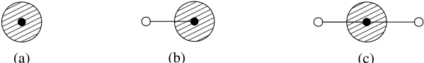
Figure 4: Graphical representation of $gV(\Phi)$, $gV^{\prime}(\Phi)$ and $gV^{\prime\prime}(\Phi)$.

As we have seen above $gV(\Phi)$ generates trees with one marked vertex, $gV^{\prime}(\Phi)$ trees with one marked vertex which is connected to an external line. One can easily check that the $k$-th derivate of $V(\Phi)$ :

$$gV^{(k)}(\Phi)=\sum_{q=0}^{\infty}\frac{w_{q+k}}{q!}\Phi^{q}$$ (81)

generates an ensemble of trees with one marked vertex connected to $k$ external lines. The graphical representations of $gV^{(k)}(\Phi)$ for $k=0,1,2$ is depicted in figure 4.

The self-consistency equation (80) is illustrated in figure 5. The content of equation (79) emerges automatically from the comparison of figure 3 (b) and figure 4 (a).

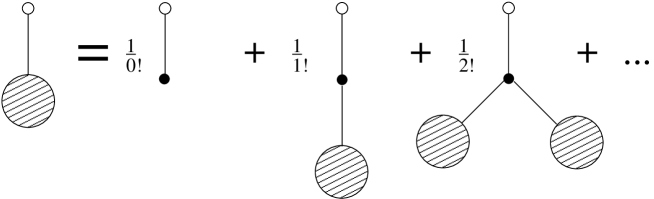
Figure 5: Graphical representation of the self-consistency equation (80).

Let us now illustrate how the generating function machinery works solving the classical problem of the tree diagram enumeration cenum . We shall calculate $z_{N}$ for the case $W_{T}=1$. This is called the Cayley problem. The number of all labeled trees with $N$ vertices is given by $z_{N}N!$. The self-consistency equation reduces to :

$$\Phi=g\>e^{\Phi}\,.$$ (82)

This equation can be solved for $\Phi$ :

$$\Phi=\sum_{N=1}^{\infty}\frac{N^{N-1}}{N!}g^{N}\>.$$ (83)

For the weights $w_{q}=1$ equation (79) leads to a simple relation between ${\cal Z}^{(1)}$ and $\Phi$ :

$${\cal Z}^{(1)}=\Phi-g=\sum_{N=2}^{\infty}\frac{N^{N-1}}{N!}g^{N}=\sum_{N=2}^{\infty}Nz_{N}g^{N}\>.$$ (84)

From this relation one can calculate the canonical partition function :

$$z_{N}=\frac{N^{N-2}}{N!}\quad\mbox{for}\quad N\geq 2$$ (85)

and the number of labeled tree diagrams to be $N^{N-2}$. For large $N$ one can approximate $z_{N}$ by :

$$z_{N}=\frac{N^{N-2}}{N!}\sim(2\pi)^{-1/2}e^{N}N^{-5/2}\sim e^{\mu_{0}N}N^{\gamma-3}\>,$$ (86)

where the last step is due to the comparison with (29). The critical value of the chemical potential and the susceptibility exponent take the values $\mu_{0}=1$ and $\gamma=1/2$, respectively. It turns out that the value $\gamma=1/2$ is a generic one. It does not change for a wide class of the weights. In the section about the universality classes and singularity types two other universality classes of branched polymer models with $\gamma\neq 1/2$ will be discussed.

We will close this appendix with the calculation of the internal two-point function. Similarly as for the partition function, it is easier to work with the generating function. Consider tree graphs which are weighted with the fugacity $g=e^{-\mu}$, and which have two marked vertices separated by $n\geq 1$ links. The generating function ${\cal G}^{(2)}\left(\mu,n\right)$ defined as a sum over all such trees corresponds to the two-point function for the grand-canonical ensemble. Figure (6) illustrates the decomposition of ${\cal G}^{(2)}\left(\mu,n\right)$ into the generating functions $gV^{\prime}(\Phi)$ and $gV^{\prime\prime}(\Phi)$ depicted in figure (4). The decomposition is unique, since the path connecting the marked vertices is unique. The two bubbles at the ends of the chain correspond to diagrams of the generating function $gV^{\prime}(\Phi)$, while the $n-1$ ones in between to $gV^{\prime\prime}(\Phi)$. The decomposition leads to the following relation :

$${\cal G}^{(2)}\left(\mu,n\right)=e^{-\left(n+1\right)\mu}\left[V^{\prime}\left(\Phi\right)\right]^{2}\cdot\left[V^{\prime\prime}\left(\Phi\right)\right]^{\left(n-1\right)}\>.$$ (87)

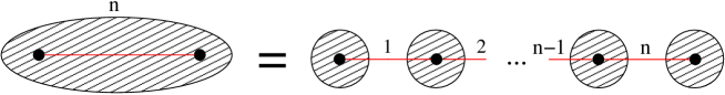
Figure 6: Decomposition of the internal two-point function ${\cal G}^{(2)}\left(\mu,n\right)$.

We can also define the internal grand-canonical two-point function for $n=0$. In this case the two marked vertices lie on top of each other. Thus the two-point function reduces to the one-point function : ${\cal G}^{(2)}\left(\mu,n=0\right)={\cal Z}^{(1)}=e^{-\mu}V(\Phi)$.

Relation (87) allows us to find an explicit dependence of the grand-canonical two-point function on $n$ and $\mu$, if we first solve the self-consistency equation (30) for $\Phi(\mu)$. We will be rather interested in the scaling behaviour of the two-point function near the critical point.

Let us first illustrate the calculation of the two-point function for the ensemble of trees having the natural weight $W_{T}=1$. In this case $V^{\prime}(\Phi)=V^{\prime\prime}(\Phi)=e^{\Phi}$, where $\Phi(\mu)$ is a solution of equation (30) :

$$\mu=\Phi-\log(\Phi)\,.$$ (88)

In this case the two-point function simplifies to :

$${\cal G}^{(2)}\left(\mu,n\right)=\exp\left(-(n+1)\left(\mu-\Phi(\mu)\right)\right)=\Phi^{n+1}\>.$$ (89)

The inversion of equation (88) for $\Phi$ gives $\Phi=1-\sqrt{2}\sqrt{\Delta\mu}$, when $\Delta\mu=\mu\!-\!\mu_{0}=\mu\!-\!1\rightarrow 0^{+}$. Thus the two-point function can be approximated in this limit by :

$${\cal G}^{(2)}\left(\mu,n\right)\sim\exp\left(-\sqrt{2}(n+1)\sqrt{\Delta\mu}\right)\>.$$ (90)

We have neglected a term linear in $\Delta\mu$ in the exponent, because we are interested in the limit $\Delta\mu\rightarrow 0^{+}$ for which $\Delta\mu\ll\sqrt{\Delta\mu}$. What matters in this limit is the leading term in $\Delta\mu$ which is related to the large $N$-behaviour of the underlying canonical-ensemble :

$${\cal G}^{(2)}\left(\mu,n\right)=\sum_{N}{\cal G}^{(2)}_{N}\left(n\right)e^{-\mu N}=\sum_{N}e^{-\mu_{0}N}{\cal G}^{(2)}_{N}\left(n\right)e^{-\Delta\mu N}\>,$$ (91)

where ${\cal G}^{(2)}_{N}(n)$ is the two-point function for the canonical ensemble for trees of size $N$. In the last formula we split into $\mu=\mu_{0}+\Delta\mu$, where $\mu_{0}$ is the critical value of $\mu$ at which the partition function is singular. The leading terms in $\Delta\mu$ of ${\cal G}^{(2)}\left(\mu,n\right)$ are responsible for the scaling behaviour while the next-to-leading ones for finite-size corrections.

Formula (91) is a discrete Laplace transform. Since we are interested in the large $N$ behaviour of ${\cal G}^{(2)}_{N}(n)$, we can substitute the discrete by a continuous Laplace transform. The inverse transform then yields :

$${\cal G}^{(2)}_{N}\left(n\right)=e^{+\mu_{0}N}\frac{1}{2\pi i}\int^{\Delta\mu_{r}+i\infty}_{\Delta\mu_{r}-i\infty}{\rm d}\Delta\mu\ {\cal G}^{(2)}\left(\mu,n\right)e^{\Delta\mu N}\>.$$ (92)

In particular, for the case discussed here (see(90)) the exact result reads :

$${\cal G}^{(2)}_{N}\left(n\right)=(2\pi)^{-1/2}e^{N}N^{-3/2}(n\!+\!1)\exp\left(-\frac{(n\!+\!1)^{2}}{2N}\right)\>.$$ (93)

We inserted $\mu_{0}=1$ in the last formula. The normalized two-point function can be approximated by :

$$g^{(2)}_{N}(n)=\frac{{\cal G}^{(2)}_{N}\left(n\right)}{\sum_{n^{\prime}}{\cal G}^{(2)}_{N}\left(n^{\prime}\right)}\simeq\frac{cn}{N}e^{-cn^{2}/2N}\>.$$ (94)

The constant $c$ in the last formula is equal $1$. We displayed this constant, because the same formula holds for generic trees in general, but with a constant which depends on the choice of the weights.

We used two approximations in the last formula. We substituted $n+1$ by $n$. The difference between the function with $n$ and $n+1$ disappears in the large $N$-limit. Secondly, the numerator and the denominator in the normalized two-point function (94) have a common part $(2\pi)^{-1/2}e^{N}N^{-3/2}$ which does not depend on $n$. It cancels out. The remaining part : $c/N$ is a normalization constant ensuring $\sum_{n}g^{(2)}_{N}(n)=1$. For finite $N$ there will be some corrections to the normalization constant $c/N$, but these disappear exponentially in the large $N$ limit.

References

- (1) Jan Ambjørn, B. Durhuus and T. Jonsson, Quantum Geometry, Cambrige, 1997.
- (2) M.J. Bowick and A. Travesset, Phys. Rep. 344 (2001) 255.
- (3) K.J. Wiese, in Phase Transition and Critical Phenomena 19, ed. Domb and Lebowitz, Academic Press, New York, (2000), 253.
- (4) J. Ambjørn, B. Durhuus, J. Fröhlich and P. Orland, Nucl. Phys. B270 [FS16] (1986) 457.
- (5) Jan Ambjørn, B. Durhuus and T. Jonsson, Phys.Lett. B244 (1990) 403.
- (6) R. Albert and A.L. Barabasi, Rev.Mod.Phys. 74 (2002) 47.
- (7) Z. Burda, J.D. Correia and A. Krzywicki, Phys.Rev. E64 (2001) 046118.
- (8) M. Polyakov, Phys.Lett. B103 (1981) 207.
- (9) F. David, Nucl.Phys. B257 (1985) 45.
- (10) V.A. Kazakov, A.A. Migdal and I.K. Kostov, Phys.Lett. B157 (1985) 295.
- (11) J. Ambjørn and J. Jurkiewicz, Phys.Lett. B278 (1992) 42.
- (12) P. Bialas, Z. Burda, A. Krzywicki and B. Petersson, Nucl.Phys. B472 (1996) 293.
- (13) J. Ambjørn, J. Jurkiewicz and R. Loll, Phys.Rev. D64 (2001) 044011.
- (14) P. Bialas, Phys.Lett. B373 (1996) 289.
- (15) J. Jurkiewicz and A. Krzywicki, Phys.Lett. B392 (1997) 291.
- (16) P. Bialas, Nucl.Phys. B575 (2000) 645.
- (17) T. Jonsson and J. Wheater, Nucl.Phys. B515 (1998) 549-574.
- (18) P. Bialas and Z. Burda, Phys.Lett. B384 (1996) 75.
- (19) W. Krauth, H. Nicolai, and M. Staudacher, Phys.Lett. B431 (1998) 31.
- (20) N. Ishibashi, H. Kawai, Y. Kitazawa and A. Tsuchiya, Nucl. Phys. B498 (1997) 467.
- (21) H. Aoki, S. Iso, H. Kawai, Y. Kitazawa and T. Tada, Prog. Theor. Phys. 99 (1998) 713.
- (22) H. Aoki, S. Iso, H. Kawai and Y. Kitazawa, Phys. Rev. E62 (2000) 6260
- (23) J.P. Bouchaud and A. Georges, Phys. Rep. 195 (1990) 127.
- (24) W. Feller, An Introduction to Probability Theory and Its Applications, Wiley and Sons, New York, 1957.
- (25) J. Ambjørn, K.N. Anagnostopoulos, W. Bietenholz, T. Hotta and J. Nishimura, JHEP 0007 (2000) 011.
- (26) J. Ambjørn, K.N. Anagnostopoulos, W. Bietenholz, T. Hotta and J. Nishimura, JHEP 0007 (2000) 013.
- (27) J. Ambjørn, K.N. Anagnostopoulos, W. Bietenholz, F. Hofheinz, and J. Nishimura, Phys.Rev. D65 (2002) 086001.
- (28) Z. Burda, B. Petersson and J. Tabaczek, Nucl.Phys. B602 (2001) 399.
- (29) P. Bialas, Z. Burda, B. Petersson and J. Tabaczek, Nucl.Phys. B592 (2001) 391.
- (30) P. Austing and J.F. Wheater, JHEP 0102 (2001) 028.
- (31) P. Austing and J.F. Wheater, JHEP 0104 (2001) 019.
- (32) G. Vernizzi and J.F. Wheater, het-th 0206226
- (33) J. Nishimura, Phys.Rev. D65 (2002) 105012.
- (34) P. Bialas, Z. Burda and D. Johnston Nucl.Phys. B493 (1997) 505.
- (35) P. Bialas, Z. Burda, B. Petersson and J. Tabaczek, Nucl.Phys. B495 (1997) 463.
- (36) J. Ambjørn and Y. Watabiki, Nucl. Phys. B445 (1995) 129.
- (37) I.P. Goulden and D.M. Jackson, Combinatorial enumeration, Wiley and Sons, New York, 1983.
- (38) Like, for instance, a theoretical physicist performing analytical calculations.
-
(39)
In the same way one can
show that all moments of the two-point function
scale uniformly for large :
which means that the two-point function is indeed a function of the scaling argument for large . -
(40)
For the simulation
we used the exact form of with the
constants and set equal to one :
- (41) If all moments of exist, the size of the central region grows faster with . For example as for an even distribution. Therefore the gaussian regime sets in faster.