A microscopic description of the aging dynamics: fluctuation-dissipation relations, effective temperature and heterogeneities

Abstract

We consider the dynamics of a diluted mean-field spin glass model in the aging regime. The model presents a particularly rich heterogeneous behavior. In order to catch this behavior, we perform a spin-by-spin analysis for a given disorder realization. The results compare well with the outcome of a static calculation which uses the “survey propagation” algorithm of Mézard, Parisi, and Zecchina [Sciencexpress 10.1126/science.1073287 (2002)]. We thus confirm the connection between statics and dynamics at the level of single degrees of freedom. Moreover, working with single-site quantities, we can introduce a new response-vs-correlation plot, which clearly shows how heterogeneous degrees of freedom undergo coherent structural rearrangements. Finally we discuss the general scenario which emerges from our work and (possibly) applies to more realistic glassy models. Interestingly enough, some features of this scenario can be understood recurring to thermometric considerations.

The description of the off-equilibrium dynamics in aging systems is one of the major challenges in contemporary statistical mechanics. Aging systems, like spin, structural and polymeric glasses SITGES_ANGELL_STRUICK are slowly evolving, heterogeneous systems which do not reach thermal equilibrium, at low enough temperatures, on any experimental time-scale. In the last 20 years a great effort has been devoted to study the dynamics of some prototypical models, namely mean-field spin glasses DynamicsReview . These models exhibit an extremely rich behavior: slow relaxation, memory effects, aging. Important tools which have been introduced in this context are the off-equilibrium fluctuation-dissipation relation (OFDR) OFDR , and the effective temperature CUKUPE one can derive from that relation. Such an effective temperature is, roughly speaking, what would be measured by a thermometer responding on the time scale on which the system ages.

One of the weak points of the results obtained so far is that they focus on global quantities, e.g. correlation and response functions averaged over the spins. On the other hand, we expect one of the peculiar features of glassy dynamics to be its heterogeneity HETERO_EXP . For instance, correlation and response functions of a particular spin depend upon its local environment HETERO_SG . Two simple remarks are in order here: $(i)$ These spin-to-spin fluctuations are non-zero even in the thermodynamic limit; $(ii)$ They disappear when the average over quenched disorder is taken.

Moreover the present definition CUKUPE of effective temperature has some problems. Indeed it corresponds to what would be measured by a specific, properly tuned, slow thermometer, while generalizations to more generic thermometers give disagreeing results EXARTIER , still to be clarified.

In this Letter, inspired by the new approach of MEPAZE , we study the aging dynamics focusing on single-site correlation and response functions. In this way we are able to consider the heterogeneities in the system and to define a microscopic, but site-independent, effective temperature.

An interesting context for addressing these issues is provided by diluted mean-field models. In these models each spin interacts with a finite number of other spins, just as in finite-dimensional models. On the other hand, the absence of a finite-dimensional geometrical structure makes them tractable from an analytic point of view.

We consider a ferromagnetic Ising model with 3-spin interactions, defined by the Hamiltonian

$$\mathcal{H}=-\sum_{m=1}^{M}\sigma_{i_{m}}\sigma_{j_{m}}\sigma_{k_{m}}\ ,$$ (1)

where the $M$ triples $(i_{m},j_{m},k_{m})$ are chosen randomly among the $\binom{N}{3}$ possible ones. Although ferromagnetic, this model is thought to have a glassy behavior for $M>0.818\,N$, due to self-induced frustration RIWEZE .

We work on a single sample with $M=N=100$, whose largest connected component contains 96 sites. We limited ourselves to such a small sample because single-spin measures require huge statistics.

We use the “survey propagation” (SP) algorithm of Refs. MEPAZE , or better its generalization at finite temperatures FDTSS2 , to compute the free energy density $F(m,\beta)$ for our specific sample at one-step replica symmetry breaking (1RSB) level. In Fig. 1 we report the complexity $\Sigma(T)=\beta\partial_{m}F(m,\beta)|_{m=1}$. The dynamic and static temperatures are defined, respectively, as the points where a non-trivial (1RSB) solution to the cavity equations first appears, and where its complexity vanishes. From the results of Fig. 1 we get the estimates $T_{d}=0.557(2)$ and $T_{c}=0.467(2)$. In the standard picture, the aging dynamics for discontinuous spin glasses is dominated by “threshold” metastable states DynamicsReview . The corresponding 1RSB parameter $m_{\rm th}(T)$ can be computed by imposing the condition $\partial_{m}^{2}[mF(m,\beta)]=0$. We computed $m_{\rm th}(T)$ on our sample for some temperatures below $T_{d}$, and in the zero temperature limit, $m_{\rm th}(T)=\mu_{\rm th}T$, with $\mu_{\rm th}=1.08(1)$. These results are summarized in the inset of Fig. 1.

Figure 1: The complexity $\Sigma$ and the 1RSB parameter for threshold states $m_{\rm th}$ (Inset) versus the temperature for the sample studied in this paper. The continuous line in the inset is the polynomial fit $m_{\rm th}(T)=1.08\,T+0.038\,T^{2}+2.17\,T^{3}$.

Another important outcome from the SP algorithm is the value of the local Edwards-Anderson order parameter $q_{\rm EA}^{(i)}(m)$, which depends on the 1RSB parameter $m$. On threshold states, the local order parameter is connected to the single-site correlation function (defined below):

$$q_{\rm th}^{(i)}\equiv q_{\text{EA}}^{(i)}(m_{\rm th})=\lim_{t\to\infty}\lim_{t_{w}\to\infty}C_{i}(t_{w}+t,t_{w})\ .$$ (2)

We consider Metropolis dynamics starting from random initial conditions, $\sigma_{i}(t\!=\!0)\!=\!\pm 1$. After a time $t_{w}$ we turn on a small random magnetic field, $h_{i}=\pm h_{0}$, and we measure single-spin correlation and integrated response functions

$$C_{i}(t_{w}+t,t_{w}) \equiv \frac{1}{t}\sum_{t^{\prime}=t}^{2t-1}\langle\sigma_{i}(t_{w}+t^{\prime})\sigma_{i}(t_{w})\rangle\ ,$$ (3)

$$\chi_{i}(t_{w}+t,t_{w}) \equiv \frac{1}{th_{0}}\sum_{t^{\prime}=t}^{2t-1}\langle\sigma_{i}(t_{w}+t^{\prime})\text{sign}(h_{i})\rangle\,,$$ (4)

where $\langle\cdot\rangle$ denotes the average over the Metropolis trajectories and the random perturbing field. The sums over $t^{\prime}$ are introduced in order to reduce the statistical error. This “experiment” is repeat $N_{\text{runs}}$ times, each time with a different thermal noise and perturbing field. Typical values for $N_{\text{runs}}$ range between $10^{6}$ and $5\cdot 10^{6}$.

The first remark on the numerical data, is that the spins can be clearly classified in two groups. Type-I spins behave as if the system were in equilibrium: the corresponding correlation and response functions satisfy time-translation invariance and the fluctuation dissipation theorem (FDT). Type-II spins are out of equilibrium spins: their correlation and response functions are non-homogeneous on long time scales and violate FDT.

Type-I includes isolated sites, but also 12 non-isolated sites. Remarkably these sites are the ones for which the SP algorithm returns $q^{(i)}_{\rm th}=0$, i.e. they are paramagnetic from the static point of view. These sites can also be identified via a simple algorithm LEAF_REM .

Figure 2: The correlation function and the $\chi$-vs-$C$ plot for the spin $i=0$ at $T=0.5$, which has $q_{\rm th}^{(0)}=0.716(7)$ (dashed line, top). Bold line (bottom) is the static $\chi_{0}[C]$ curve.

Let us hereafter focus on type-II spins, that is on glassy degrees of freedom. In Fig. 2 we show the correlation function for a generic type-II spin ($i=0$ here) and the corresponding $\chi$-vs-$C$ plot. For this spin we have $q_{\rm th}=0.716(7)$, shown with a dashed line in Fig. 2 (top). In the limit of very large times we expect (in analogy with OFDR ) the OFDR $\chi_{i}(t,t^{\prime})=\chi_{i}[C(t,t^{\prime})]$ to hold. Moreover the function $\chi_{i}[C]$ should be related to static quantities FMPP . Numerical data, for this and for all the other spins, seem to converge to the static curve $\chi_{i}[C]$. This is an evidence for a strong link between static and dynamic observables even at the level of single degrees of freedom.

The 1RSB static calculation yields

$$T\;\chi_{i}[C]=[1-C]\;\theta\left(C-q_{\rm th}^{(i)}\right)+\\ +\left[1-q_{\rm th}^{(i)}-m_{\rm th}\left(C-q_{\rm th}^{(i)}\right)\right]\;\theta\left(q_{\rm th}^{(i)}-C\right)\,.$$ (5)

The OFDR changes from site to site because the $q_{\rm th}^{(i)}$ changes. Note, however, that the $\chi_{i}[C]$ curves are parallel in the aging regime, since $m_{\rm th}$ only depends on the temperature (cf. Fig. 3).

Figure 3: In the $\chi$-vs-$C$ plot for seven generic sites at $T=0.3$ system heterogeneities become apparent. The seven data sets can be nicely collapsed with no fitting parameters (bottom).

System heterogeneities manifest themselves in the large variability of the $q_{\rm th}^{(i)}$ local order parameters. The $\chi$-vs-$C$ plot for seven generic sites, see Fig. 3 (top), clearly shows this variability. In order to check that single-site data can be well described by Eq. (5) we rescale data of Fig. 3 using the scaling variables $C_{i}^{\rm res}=1-A_{i}(1-C_{i})$ and $\chi_{i}^{\rm res}=A_{i}\chi_{i}$, where $A_{i}=(1-\overline{q})/(1-q_{\rm th}^{(i)})$, $\overline{q}$ being a reference overlap which can be chosen freely. Rescaled data are shown in Fig. 3 (bottom).

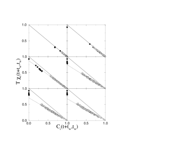
Figure 4: The “movie” plot: Evolution of the single-spin correlation and response functions in the $(C,\chi)$ plane. Here we use $h=0.1$, $T=0.4$, and $t_{w}=10^{5}$. Different frames correspond to (from left to right and up to bottom): $t=2^{4}$, $2^{9}$, $2^{12}$, $2^{15}$, $2^{16}$, and $2^{17}$. Black and white circles refer, respectively, to type-I and type-II sites. Black circles are not exactly on the FDT line because of finite-$h_{0}$ effects, to be discussed in Ref. FDTSS2 . Dotted lines are fits to the white data.

A last important question, in order to complete the description of the time evolution of single-site quantities, regards the time law with which spin $i$ runs along the curve $\chi_{i}[C]$. The answer to this question is very surprising and it is shown in Fig. 4, where we plot the time evolution of all the 100 $C_{i}$’s and $\chi_{i}$’s.

Amazingly, sites-II data leave the FDT line coherently (when the system undergoes a global structural rearrangement) and they remain very well aligned for later times. Fits to a function

$$\chi_{i}(t_{w}+t,t_{w})=\frac{1-C_{i}(t_{w}+t,t_{w})}{T_{\rm fit}(t_{w},t)}$$ (6)

give very accurate results with $T_{\rm fit}=0.459$ (for $t=2^{12}$), $0.536$ ($t=2^{15}$), $0.564$ ($t=2^{16}$), $0.590$ ($t=2^{17}$).

In the following discussion we shall try to outline a few general properties which can be extrapolated from our numerical results, and, possibly, applied to a wider variety of systems. Our basic objects are the local correlation and response functions $C_{i}(t,t^{\prime})$ and $R_{i}(t,t^{\prime})\equiv-\partial_{t^{\prime}}\chi_{i}(t,t^{\prime})$. Following Refs. OFDR , we guess that $\partial_{t}C_{i}(t,t^{\prime}),\,\partial_{t}R_{i}(t,t^{\prime})\leq 0$, and $\partial_{t^{\prime}}C_{i}(t,t^{\prime}),\,\partial_{t^{\prime}}R_{i}(t,t^{\prime})\geq 0$. Moreover $C_{i}(t,t^{\prime}),\,R_{i}(t,t^{\prime})\!\to\!0$ as $t\!\to\!\infty$ for any fixed $t^{\prime}$. All these properties are well realized within our model.

The first non-trivial property  is that, for any “non-exceptional” pair of spins $i$ and $j$ there exist two continuous functions $f_{ij}$ and $f_{ji}$ such that

$$C_{i}(t,t^{\prime})=f_{ij}[C_{j}(t,t^{\prime})]\ ,\quad C_{j}(t,t^{\prime})=f_{ji}[C_{i}(t,t^{\prime})]\ ,$$ (7)

asymptotically for $t,t^{\prime}\gg 1$. We shall not specify what does “non-exceptional” mean , but the reader is urged to bear in mind the example of type-I (paramagnetic) spins in our model: if $i$ is type-I, and $j$ is type-II, then relation (7) clearly does not hold.

It is easy to show that transition functions $\{f_{ij}\}$ can be written in the form $f_{ij}=f_{i}^{-1}\circ f_{j}$. Of course the functions $f_{i}$ are not unique: in particular they can be modified by a global reparametrization $f_{i}\to g\circ f_{i}$.

Moreover Eq. (7) implies a one-to-one correspondence between the correlation scales (in the sense of OFDR ) of sites $i$ and $j$. Notice that, for our model, this is unavoidable if we want the connection between statics and dynamics to be satisfied both at the level of global and local (single-spin) observables. Physically this first property means that structural rearrangements occurs coherently in the whole system. Notice that this is not unphysical, because far apart degrees of freedom are coherent only on a coarse time resolution (diverging with $t_{w}$).

The second property has been illustrated at length above: For large times $t,t^{\prime}$, a local OFDR of the form $\chi_{i}(t,t^{\prime})=\chi_{i}[C_{i}(t,t^{\prime})]$ exists (the connection with the static result is not a crucial point here).

Our third property determines the form of the transition functions $f_{ij}=f_{i}^{-1}\circ f_{j}$ in the aging regime. In fact the results in Fig. 4 suggest that

$$\frac{\chi_{i}(t,t^{\prime})}{1-C_{i}(t,t^{\prime})}=\frac{\chi_{j}(t,t^{\prime})}{1-C_{j}(t,t^{\prime})}\quad\forall\ i,j\ .$$ (8)

Combined with the OFDR, this means that we can take $f_{i}[C]=\chi_{i}[C]/(1-C)$ for $C<q_{\rm th}^{(i)}$. This relation cannot be extended to the quasi-equilibrium regime $C_{i}>q_{\rm th}^{(i)}$, because we would obtain $f_{i}[C]=\beta$ identically, which is not invertible.

Finally the fourth property is:

$$\chi_{i}^{\prime}[C_{i}(t,t^{\prime})]=\chi_{j}^{\prime}[C_{j}(t,t^{\prime})]\ ,$$ (9)

or, in other words $\chi_{i}^{\prime}[C_{i}]=\chi_{j}^{\prime}[C_{j}]$ when $C_{i}=f_{ij}[C_{j}]$. Notice that, for our model, this property is satisfied by the prediction we draw from the statics. However, a direct numerical verification is quite hard.

Suppose now to measure the temperature of the spin $i$, by weakly coupling it to a thermometer . If the thermometer respond quickly, it measures the bath temperature $T$ for any site $i$, independently of the details of the thermometer itself. However, if the thermometer is “slow”, it measures an effective temperature $T_{\rm meas}>T$, which depends upon the specific thermometer used EXARTIER . Nevertheless, the above scenario imply FDTSS2 that $T_{\rm meas}$ is site-independent. The converse is also true: if one of the above four properties ceases to hold, one can construct a thermometer which distinguishes colder sites from hotter ones, and use it to transfer heat.

Our conclusions are summarized in Fig. 5. Dynamical heterogeneities turn out to be strongly constrained in the aging regime. These constraints can be derived from the hypothesis of thermometric indistinguishability of different sites FDTSS2 .

We are deeply indebted with Riccardo Zecchina and Marc Mézard, who discussed with us their results MEPAZE before publication. A. M. thanks Leticia Cugliandolo and Jorge Kurchan for their interest in this work, and the ESF for financial support.

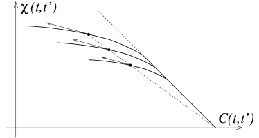
Figure 5: A pictorial view of heterogeneous aging dynamics. It is sufficient to know the dynamics of a single spin in the system, in order to reconstruct the behavior of any other one (once the static parameters $q_{\rm th}^{(i)}$ are known).

References

- (1) E. Vincent et al., in Proceedings of the Sitges conference (M. Rubi ed., Springer-Verlag, 1997). C.A. Angell, Science 167, 1924 (1995). L.C.E. Struick, Physical aging in amorphous polymers and other materials (Elsevier,1978).
- (2) J.-P. Bouchaud et al., in Spin Glasses and Random Fields, A.P. Young ed. (World Scientific, 1997).
- (3) L.F. Cugliandolo and J. Kurchan, Phys. Rev. Lett. 71, 173 (1993); J. Phys. A 27, 5749 (1994).
- (4) L.F. Cugliandolo, J. Kurchan and L. Peliti, Phys. Rev. E 55, 3898 (1997).
- (5) M.D. Ediger, Annu. Rev. Phys. Chem. 51, 99 (2000). W.K. Kegel and A. van Blaaderen, Science 287, 290 (2000). E.R. Weeks et al., Science 287, 627 (2000).
- (6) P.H. Poole et al., Phys. Rev. Lett. 78, 3394 (1997). A. Barrat and R. Zecchina, Phys. Rev. E 59, R1299 (1999). F. Ricci-Tersenghi and R. Zecchina, Phys. Rev. E 62, R7567 (2000). H.E. Castillo et al., Phys. Rev. Lett. 88, 237201 (2002).
- (7) R. Exartier and L. Peliti, Eur. Phys. J. B 16, 119 (2000).
- (8) M. Mézard, G. Parisi and R. Zecchina, Sciencexpress 10.1126/science.1073287 (2002). M. Mézard and R. Zecchina, cond-mat/0207194.
- (9) A. Montanari and F. Ricci-Tersenghi, to appear.
- (10) F. Ricci-Tersenghi, M. Weigt, and R. Zecchina, Phys. Rev. E 63, 026702 (2001)
- (11) S. Cocco et al., cond-mat/0206239. M. Mézard, F. Ricci-Tersenghi, and R. Zecchina, cond-mat/0207140.
- (12) S. Franz, M. Mézard, G. Parisi, and L. Peliti, Phys. Rev. Lett. 81, 1758 (1998); J. Stat. Phys. 97, 459 (1999).