Doping dependence of the spin gap in a 2-leg ladder

Abstract

A spin-fermion model relevant for the description of cuprates ladders is studied in a path integral formalism, where, after integrating out the fermions, an effective action for the spins in term of a Fermi-determinant results. The determinant can be evaluated in the long-wavelength, low-frequency limit to all orders in the coupling constant, leading to a non-linear $\sigma$ model with doping dependent coupling constants. An explicit evaluation shows, that the spin-gap diminishes upon doping as opposed to previous mean-field treatments.

I Introduction

Doped quantum antiferromagnets (QAFM) constitute a major unresolved problem in condensed matter physics, which is at the center of current research since the discovery of high $T_{c}$ superconductivity Bednorz and Müller (1986). In particular, the case of a doped spin liquid –where no symmetry is spontaneously broken– is very challenging, since the starting point, the spin liquid state, cannot be described by a classical Néel state.

This problem is not only of theoretical relevance. $\textrm{Cu}_{2}\textrm{O}_{3}$ ladders are present in $\textrm{Sr}_{14-x}\textrm{Ca}_{x}\textrm{Cu}_{24}\textrm{O}_{41}$ and many experiments support the presence of a spin gap and a finite correlation length Kumagai et al. (1997); Magishi et al. (1988); Carretta et al. (1998); Eccleston et al. (1998); Katano et al. (1999); Gozar et al. (2001), two crucial ingredients signaling a spin liquid state. With isovalent $\textrm{Ca}^{2+}$ substitution of $\textrm{Sr}^{2+}$ holes are transferred from the $\textrm{CuO}_{3}$ chains to the ladders Osafune et al. (1997), increasing the conductivity of the latter. The spin gap, as measured by Knight shift or NMR experiments Kumagai et al. (1997); Magishi et al. (1988); Carretta et al. (1998) is seen to diminish. With increasing doping, superconductivity is ultimately stabilized under pressure Mayaffre et al. (1998); Piskunov et al. (2000), a phenomenon that suffices to justify the interest for the subject.

The simplest model which is believed to grasp the physics of the problem is the $t-J$ model on a two leg ladder. It is believed in general that this system evolves continuously from the isotropic case to the limit of strong rung interaction. In this limit some simplifying pictures are at hand: without doping the gap is the energy of promoting a singlet rung to a triplet ($\sim J_{\perp}$). Interaction among the rungs leads eventually to the usual magnon band. Upon doping the systems shows two different kinds of spin excitations Tsunetsugu et al. (1994); Troyer et al. (1996). One is still the singlet-triplet transition as before, the other kind corresponds to the splitting of a hole pair into a couple of quasiparticles (formed by a spinon and an holon), each carrying charge $+\left|e\right|$ and spin 1/2. The number of possible excitations is proportional to $\left(1-\delta\right)$ (for the magnons) and $\delta$ (for the quasiparticles), respectively, where $\delta$ is the number of holes per copper sites. For this reason, at low doping concentration, the magnon gap will be the most important in influencing the form of the static susceptibility or dynamical structure factor.

First Sigrist et. al.  Sigrist et al. (1994) and more recently Lee et. al. Lee et al. (1999) attacked the problem ultimately with some sort of mean field decoupling. Their results agree in predicting an increase of the magnon gap ($\Delta_{M}$, originated from the singlet-triplet transition), while Lee et. al. were also able to calculate a decrease of the quasiparticle gap ($\Delta_{QP}$ originated from the splitting of a hole pair) for small doping concentrations.

In contrast to the mean-field results above, Ammon et. al.  Ammon et al. (1999) obtained a decrease of the magnon gap and an almost doping independent $\Delta_{QP}$ using temperature density matrix renormalization group (TDMRG). As already mentioned, a decrease of the spin gap is also observed in a number of experiments Kumagai et al. (1997); Magishi et al. (1988); Carretta et al. (1998).

In this paper we concentrate on the behavior of the magnon gap upon doping. Due to the contradiction above it is imperative to go beyond mean field and include the role of fluctuations in a controlled manner. A mapping from an AFM Heisenberg model to an effective field theory, the non linear $\sigma$ model (NL$\sigma$M), proved very efficient in describing the magnetic properties of two dimensional spin lattices Chakravarty et al. (1988), chains Haldane (1983), and ladders Dell’Aringa et al. (1997). This mapping was extended in Ref. Muramatsu and Zeyher (1990) to the case of a doped two dimensional QAFM using a procedure that we will closely follow.

II Mapping to an effective spin action

Since no satisfactory analytical treatment of the $t-J$ model away from half filling is possible at present, we focus on the so called spin-fermion model. This Hamiltonian can be derived in fourth order degenerate perturbation theory Zaanen and Oleś (1988); Muramatsu et al. (1988) from the $p-d$, three band, Emery model Emery (1987), that gives a detailed description of the cuprate materials. There the role of perturbation is played by the hybridization term between the $p$-orbital (oxygen) and the $d$-orbital (copper). A further simplification of the model was proposed by Zhang and Rice Zhang and Rice (1988), that leads to the $t-J$ model.

A typical copper-oxide two leg ladder, as those present in $\textrm{Sr}_{14-x}\textrm{Ca}_{x}\textrm{Cu}_{24}\textrm{O}_{41}$ is depicted in Fig. 1. It is generally accepted that the dopant holes reside on p-orbitals on the oxygens sites, whereas on the $\textrm{Cu}^{2+}$ ions a localized hole resides, represented by spin 1/2 operator which interact via a nearest neighbor exchange.

Figure 1: Schematic picture of a two leg ladder Copper-Oxide.

The spin-fermion Hamiltonian is defined as follows:

$$H_{SF} = t\sum_{\left\langle j,j^{\prime};i\right\rangle,i,\sigma}\left(-1\right)^{\alpha_{i,j}+\alpha_{i,j^{\prime}}}c^{{{\dagger}}}_{j,\sigma}c_{j^{\prime},\sigma}+J_{K}\sum_{i}\mathbf{R}_{i}\cdot\mathbf{S}_{i}$$ (1)

$$+J_{H}\sum_{\left\langle i,i^{\prime}\right\rangle}\mathbf{S}_{i}\cdot\mathbf{S}_{i^{\prime}}.$$

The index $i$ ($j$) runs over the Cu (O) sites, $c^{{{\dagger}}}_{j,\sigma}$ creates a hole in an oxygen $p$ band and $\mathbf{S}_{j}$ are spin operators for the copper ions. The coefficients $\alpha_{i,j}$ take care of the sign of the p-d overlap and $\alpha_{i,j}=1$ if $j=i+\frac{1}{2}\hat{x}$ or $i+\frac{1}{2}\hat{y}$ and $\alpha_{i,j}=2$ if $j=i-\frac{1}{2}\hat{x}$ or $i-\frac{1}{2}\hat{y}$. Finally the operator $\mathbf{R}_{i}$ is defined as

$$\mathbf{R}_{i}=\sum_{\left\langle j,k;i\right\rangle,i,\alpha,\beta}(-1)^{\alpha_{i,j}+\alpha_{i,k}}c^{{{\dagger}}}_{j,\alpha}\mbox{\large\boldmath$\sigma$}_{\alpha,\beta}c_{k,\beta}.$$ (2)

Following Zhang and Rice (1988) we can define the following operator centered on the copper site $P_{i,\sigma}=\left(1/2\right)\sum_{\left\langle j;i\right\rangle}\left(-1\right)^{\alpha_{i,j}}c_{j,\sigma}$ which represents non orthogonal orbitals with a high weight on the $i$ site. Their anti-commutation relations are

$$\left\{P_{i,\sigma},P^{{{\dagger}}}_{i^{\prime},\sigma^{\prime}}\right\}=\delta_{\sigma,\sigma^{\prime}}\left(\delta_{i,i^{\prime}}-\frac{1}{4}\delta_{\left\langle i,i^{\prime}\right\rangle}\right),$$ (3)

and we can rewrite the Hamiltonian in terms of these operators as follows

$$H_{SF} = 4t\sum_{\begin{subarray}{c}l=1\ldots L\\ \lambda=1,2,\sigma\end{subarray}}P_{l,\lambda,\sigma}^{{{\dagger}}}P_{l,\lambda,\sigma}+4J_{K}\sum_{\begin{subarray}{c}l=1\ldots L\\ \lambda=1,2,\alpha,\beta\end{subarray}}P_{l,\lambda,\alpha}^{{{\dagger}}}\mbox{\large\boldmath$\sigma$}_{\alpha,\beta}P_{l,\lambda,\beta}\cdot\mathbf{S}_{l,\lambda}$$ (4)

$$+J_{\perp}\sum_{l=1\ldots L}\mathbf{S}_{l,1}\cdot\mathbf{S}_{l,2}+J_{||}\sum_{\begin{subarray}{c}l=1\ldots L\\ \lambda=1,2\end{subarray}}\mathbf{S}_{l,\lambda}\cdot\mathbf{S}_{l+1,\lambda},$$

$L$ is the number of the rungs along the ladder and $\lambda=1,2$ distinguishes the two legs. For the sake of generality, an anisotropy in the Heisenberg term is allowed.

The different steps of our procedure are the following: first find orthogonal (Wannier states) for the holes, then go to a (coherent states) path integral formulation for spins and fermions and perform the Gaussian integration of the fermionic degrees of freedom. The remaining part of the calculation is devoted to the evaluation of the resulting Fermi determinant in the long-wavelength low-frequency limit. This expansion includes the coupling constant $J_{K}$ to all order.

Wannier states are easily find via $P_{\mathbf{k},\sigma}=\sqrt{\epsilon(\mathbf{k})}f_{\mathbf{k},\sigma}$where $\epsilon\left(\mathbf{k}\right)=\left(1-\frac{\cos\left(k_{x}a\right)+\cos\left(k_{y}a\right)/2}{2}\right)$. Here $a$ is the lattice constant and we used a two dimensional Fourier transform where $k_{y}$ takes only values $0$ and $\pi/a$ distinguishing between symmetric (bonding) and antisymmetric (antibonding) states. The partition function can be expressed as a path integral

$$Z=\int D\left[f^{\ast}\right]D\left[f\right]D[\hat{\Omega}]e^{-S_{SF}},$$ (5)

where $S_{SF}=S_{h}+S_{s}$. The action $S_{s}$ contains all terms with spins degree of freedoms only Dombre and Read (1988):

$$S_{s}=\int^{\beta}_{0}d\tau\left[-iS\sum_{l,\lambda}\mathbf{A}\left(\hat{\Omega}_{l,\lambda}\right)\cdot\frac{\partial\hat{\Omega}_{l,\lambda}}{\partial\tau}+H_{\textrm{Heis}}\left(S\hat{\Omega}\left(\tau\right)\right)\right],$$ (6)

where $\hat{\Omega}$ is a unimodular field, $S$ is the spin per site ($1/2$ in our case) and $\mathbf{A}$ is the vector potential for a (Dirac) monopole: $\epsilon^{abc}(\partial A_{a}/\partial\hat{\Omega}_{b})=\hat{\Omega}_{c}$.

It is by now well accepted that the effective low energy field theory of the $d$-dimensional Heisenberg antiferromagnetic model is given by the $(d+1)$ NL$\sigma$M Haldane (1983); Affleck (1989); Auerbach (1994). In the case of a ladder one obtains the $(1+1)$ NL$\sigma$M Dell’Aringa et al. (1997); Sierra (1996). For this reason, here we will deal mainly with the part of the action which contains fermionic degrees of freedom $S_{h}$:

$$S_{h}=\sum_{kq\alpha\beta}f_{k,\alpha}^{\ast}\left[\left(i\omega_{n}+4t\epsilon\left(\mathbf{k}\right)-\mu\right)\delta_{k,q}\delta_{\alpha,\beta}+g\sqrt{\epsilon\left(\mathbf{k}\right)\epsilon\left(\mathbf{q}\right)}\mbox{\large\boldmath$\sigma$}_{\alpha,\beta}\cdot\hat{\Omega}_{k-q}\right]f_{q,\beta},$$ (7)

here $k=\left(k_{x},k_{y},\omega_{n}\right)$ where $\omega_{n}=\pi\left(2n+1\right)/\beta$ are the fermionic Matsubara frequency and $g=4J_{K}S$. It is natural to decompose the inverse propagator into $G^{-1}=G_{0}^{-1}-\Sigma$ where the free part is

$$G_{0}^{-1}=\left(i\omega_{n}+4t\epsilon(\mathbf{k})-\mu\right)\delta_{k,q}\delta_{\alpha,\beta},$$ (8)

and the fluctuating external potential is

$$\Sigma=-g\sqrt{\epsilon(\mathbf{k})\epsilon(\mathbf{q})}\mbox{\large\boldmath$\sigma$}_{\alpha,\beta}\cdot\hat{\Omega}_{k-q}.$$ (9)

Since, according to Eq. (7) the action $S_{SF}$ is bilinear in the fermionic variables, we can integrate them out. This leads to $S_{SF}=S_{s}-\mathrm{tr}\ln G^{-1}$. Defining the matrix

$$A=\sqrt{\epsilon\left(\mathbf{k}\right)}\delta_{k,q}\delta_{\alpha,\beta}$$ (10)

and a rescaled propagator $\hat{G}^{-1}$ through

$$\hat{G}^{-1}={A^{{{\dagger}}}}^{-1}G^{-1}A^{-1}$$ (11)

we can write

$$\mathrm{tr}\ln\left(G^{-1}\right)=\mathrm{tr}\ln\left(AA^{{{\dagger}}}\right)+\mathrm{tr}\ln\left(\hat{G}^{-1}\right),$$ (12)

the first term gives just a constant and we can ignore it. Again we decompose the rescaled inverse propagator as $\hat{G}^{-1}=\hat{G}^{-1}_{0}-\hat{\Sigma}$ which brings us to

$$\hat{G}^{-1}_{0} = \left(\frac{i\omega_{n}+4t\epsilon\left(\mathbf{k}\right)-\mu}{\epsilon\left(\mathbf{k}\right)}\right)\delta_{kq}\delta_{\alpha\beta}\equiv g_{0}^{-1}\left(k_{x},k_{y},\omega_{n}\right)\delta_{k,q}\delta_{\alpha,\beta},$$ (13)

$$\hat{\Sigma} = -g\Omega_{\mathbf{k}-\mathbf{q},\omega-\nu}\cdot\mbox{\large\boldmath$\sigma$}_{\alpha\beta}.$$ (14)

The remaining part of the calculation is devoted to the evaluation of $S_{h\textrm{ eff}}=-\mathrm{tr}\ln\left(\hat{G}^{-1}\right)$ in the continuum limit.

II.1 Parameterizations

As we already mentioned, in the undoped regime where no holes are present, it has proven very effective a mapping from a antiferromagnetic Heisenberg spin ladder to a (1+1) NL$\sigma$M. This mapping rely on the idea that although long range order (here antiferromagnetic) is prohibited in one dimension, the most important contribution to the action are given by paths in which antiferromagnetic order survives at short distance. Accordingly the dynamical unimodular field is decomposed in a Néel modulated field $\mathbf{n}$ plus a ferromagnetic fluctuating contribution. A gradient expansion in the dynamical field brings then to the (1+1) NL$\sigma$M. The gradient expansion is justified when the correlation length of the spin is much larger than the lattice constant $a$. However the prediction of the NL$\sigma$M, i. e. a finite correlation length and a triplet of massive modes above the ground state Haldane (1983); Polyakov (1975); Polyakov and Weigman (1983); Shankar and Read (1990) remain valid until $\xi\approx 2.5a$ as numerical calculations on the isotropic Heisenberg ladder have shown White et al. (1994).

The basic assumption of this work is then that such a parameterization is still meaningful as long as the spin liquid state is not destroyed by doping, as seems to be the case in experiments, where a finite spin-gap is also seen in the doped case Kumagai et al. (1997); Magishi et al. (1988); Carretta et al. (1998); Eccleston et al. (1998); Katano et al. (1999); Gozar et al. (2001). Then, as e.g. in ref. Dombre and Read (1988), we parameterize the spin field in the following way

$$\Omega_{i,\lambda}\left(\tau\right)=\left(-1\right)^{i+\lambda}\mathbf{n}_{i,\lambda}\sqrt{1-\left|\frac{a\mathbf{l}_{i,\lambda}}{S}\right|^{2}}+\frac{a\mathbf{l}_{i,\lambda}}{S},$$ (15)

$\mathbf{n}_{i,\lambda}$ and $\mathbf{l}_{i,\lambda}$ are two slowly varying, orthogonal, vector fields describing locally antiferromagnetic and ferromagnetic configurations, respectively. $\mathbf{n}_{i,\lambda}$ is normalized such that $|\mathbf{n}_{i,\lambda}|^{2}=1$. The lattice constant $a$ in front of $\mathbf{l}_{i,\lambda}$ in eq. (15) makes explicit the fact that $\mathbf{l}_{i,\lambda}$ is proportional to a generator of rotations of $\mathbf{n}_{i,\lambda}$, namely to a first-order derivative of $\mathbf{n}_{i,\lambda}$.

In the particular geometry of a ladder, this decomposition give rise to two local order parameters, $\mathbf{n}_{i,1}$ and $\mathbf{n}_{i,2}$. However we assume that spins across the chain are rather strongly correlated such that they will sum up to give rise to an antiferromagnetic configuration, or subtract and give a ferromagnetic fluctuation. A further parameterization is then

$$\mathbf{n}_{i,\lambda}=\mathbf{N}_{i}\sqrt{1-a^{2}\left|\mathbf{M}_{i}\right|^{2}}+\left(-1\right)^{\lambda}a\mathbf{M}_{i},$$ (16)

with $\mathbf{N}_{i}\cdot\mathbf{M}_{i}=0$ and $|\mathbf{N}_{i}|^{2}=1$.

The next step is the gradient expansion, or equivalently, in Fourier space, an expansion in powers of $k$. In (1+1) dimensions the field $\mathbf{N}$ will get no scaling dimension, whereas the fields $\mathbf{l}$ and $\mathbf{M}$ get scaling dimension -1. Accordingly, in the subsequent expansion we will need to keep terms with up to two derivative and any power of the field $\mathbf{N}$. Terms containing $\mathbf{l},\mathbf{M}$ are marginal whenever two fields or one field and one derivative are present. Higher order terms are irrelevant and will be discarded. This correspond to expand all our quantities up to $O\left(a^{2}\right)$.

The self energy has then the following expansion

$$\hat{\Sigma}=\Sigma_{00}+\Sigma_{01}+\Sigma_{02}+\Sigma_{1}+\Sigma_{2}+O\left(a^{3}\right),$$ (17)

where the various quantity are

$$\Sigma_{00} = -g\delta_{k_{y}-q_{y},\pi}\,\mathbf{N}_{k_{x}-q_{x}+\pi,\omega-\nu}\cdot\mbox{\large\boldmath$\sigma$}_{\alpha\beta},$$ (18)

$$\Sigma_{01} = -ag\delta_{k_{y}-q_{y},0}\,\mathbf{M}_{k_{x}-q_{x}+\pi,\omega-\nu}\cdot\mbox{\large\boldmath$\sigma$}_{\alpha\beta},$$ (19)

$$\Sigma_{02} = \frac{a^{2}g}{2}\delta_{k_{y}-q_{y},\pi}\,\left(\mathbf{N}\left|\mathbf{M}\right|^{2}\right)_{k_{x}-q_{x}+\pi,\omega-\nu}\cdot\mbox{\large\boldmath$\sigma$}_{\alpha\beta},$$ (20)

$$\Sigma_{1} = -\frac{ag}{S}\mathbf{l}_{\mathbf{k}-\mathbf{q},\omega-\nu}\cdot\mbox{\large\boldmath$\sigma$}_{\alpha\beta},$$ (21)

$$\Sigma_{2} = \frac{a^{2}g}{2S^{2}}\left(\mathbf{N}\left|\mathbf{l}\right|^{2}\right)_{\mathbf{k}-\mathbf{q}+\mathbf{Q},\omega-\nu}\cdot\mbox{\large\boldmath$\sigma$}_{\alpha\beta},$$ (22)

where $\mathbf{Q}=\left(\pi/a,\pi/a\right)$ is the antiferromagnetic modulation vector suitable for a ladder geometry. We also regroup the zero-th order term in $F^{-1}\equiv\hat{G}_{0}^{-1}-\Sigma_{00}$.

The evaluation of the various contribution in the continuum limit, proceeds very similarly as in ref. Muramatsu and Zeyher (1990), and we refer to that paper for a more detailed explanation. The quantity to be evaluated is

$$S_{h\textrm{ eff}}=-\mathrm{tr}\ln\left(F^{-1}\right)-\mathrm{tr}\ln\left(1\negthickspace{\rm I}-F\left(\Sigma_{01}+\Sigma_{02}+\Sigma_{1}+\Sigma_{2}\right)\right).$$ (23)

We need then to find the inverse of $F^{-1}$ up to $O\left(a\right)$. It turns out that

$$F=\bar{F}D^{-1}-a\bar{F}D^{-1}RD^{-1}+O\left(a^{2}\right),$$ (24)

where the various matrices are

$$\bar{F} = \bar{g}^{-1}_{0}\left(\mathbf{k},\omega\right)\delta_{kq}\delta_{\alpha\beta}-g\delta_{k_{y}-q_{y},\pi}\mathbf{N}_{k_{x}-q_{x}+\pi}\cdot\mbox{\large\boldmath$\sigma$}_{\alpha\beta},$$ (25)

$$D = D(\mathbf{k},\omega)\delta_{kq}\delta_{\alpha\beta},$$ (26)

$$R = -g\,\delta_{k_{y}-q_{y},\pi}\sum_{r=x,\tau}\left(k_{r}-q_{r}+\delta_{r,x}\pi/a\right)\,\partial_{r}g^{-1}_{0}(\mathbf{k},\omega)\mathbf{N}_{k-q+Q}\cdot\mbox{\large\boldmath$\sigma$}_{\alpha\beta},$$ (27)

and we used the shorthand notation

$$\bar{g}_{0}^{-1}\left(\mathbf{k},\omega_{n}\right) = g^{-1}_{0}\left(\mathbf{k}+\mathbf{Q},\omega_{n}\right),$$ (28)

$$D(\mathbf{k},\omega_{n}) = g^{-1}_{0}\left(\mathbf{k},\omega_{n}\right)\bar{g}_{0}^{-1}\left(\mathbf{k},\omega_{n}\right)-g^{2}.$$ (29)

We first consider the term

$$\mathrm{tr}\ln\left(F^{-1}\right)=\mathrm{tr}\ln\left(\hat{G}^{-1}_{0}\right)+\mathrm{tr}\ln\left(1\negthickspace{\rm I}-\hat{G}_{0}\Sigma_{00}\right).$$ (30)

The second term of this equation is reduced to the calculation of

$$\sum_{m=1}^{\infty}\frac{1}{n}\mathrm{tr}\left(\hat{G}_{0}\Sigma_{00}\right)^{m},$$ (31)

where each term has the following expansion

$$\mathrm{tr}\left(\hat{G}_{0}\Sigma_{00}\right)^{m} = (g)^{m}\sum_{k,q_{2}\ldots q_{m}}g_{0}(k)\bar{g}_{0}(k+q_{2})g_{0}(k+q_{3})\bar{g}_{0}(k+q_{4})\cdots g_{0}(k+q_{m-1})\bar{g}_{0}(k+q_{m})$$ (32)

$$\times\mathbf{N}^{a_{1}}_{-q_{2}}\mathbf{N}^{a_{2}}_{q_{1}-q_{2}}\cdots\mathbf{N}^{a_{2}}_{q_{m}}\mathrm{tr}\left(\sigma^{a}_{1}\sigma^{a}_{2}\cdots\sigma^{a}_{m}\right),$$

with $m$ an even integer. The trace over the Pauli matrices can be carried out using a trace reduction formula Veltman (1989). The gradient expansion in Eq. (32) is then obtained by performing an expansion of the product of propagators $g_{0}(k)\cdots\bar{g}_{0}(k+q_{m})$ in powers of the variables $q_{2},q_{3},\ldots q_{m}$ that appear as argument of the vector field $\mathbf{N}$. The result obtained is Muramatsu and Zeyher (1990)

$$\mathrm{tr}\ln\left(1\negthickspace{\rm I}-\hat{G}_{0}\Sigma_{00}\right)=\int dxd\tau\left[\frac{\bar{\chi}_{xx}}{2}\left|\partial_{x}\mathbf{N}\right|^{2}+\frac{\bar{\chi}_{\tau\tau}}{2}\left|\partial_{\tau}\mathbf{N}\right|^{2}\right],$$ (33)

with the definition

$$\bar{\chi}_{\alpha\beta}=\left.\frac{\partial^{2}}{\partial q_{\alpha}\partial q_{\beta}}\sum_{k}\ln\left[1-g^{2}g(k)g(k+q+Q)\right]\delta_{q_{y}0}\right|_{q=0}.$$ (34)

We can now pass to the evaluation of the second term in Eq. (23). This does not present particular problems, since after expanding all the quantities, it reduces to the evaluation of a finite number of traces. The result is

$$\mathrm{tr}\ln\left(1\negthickspace{\rm I}-F\left(\Sigma_{01}+\Sigma_{02}+\Sigma_{1}+\Sigma_{2}\right)\right) = i\frac{g^{3}}{S}\int\!\!dx\,d\tau\hat{\chi}_{\tau}\left(\mathbf{N}\times\partial_{\tau}\mathbf{N}\right)\cdot\left(\mathbf{l}_{1}+\mathbf{l}_{2}\right)$$ (35)

$$-\frac{g^{2}}{8S^{2}}\int\!\!dx\,d\tau\tilde{\chi}\left(\mathbf{l}_{1}+\mathbf{l}_{2}\right)^{2}.$$

Here we omitted to write a Gaussian term $\propto\mathbf{M}^{2}$, completely decoupled, which can be integrated out without further consequences. The quantities $\hat{\chi}_{\tau}$ and $\tilde{\chi}$ are given by

$$\hat{\chi}_{\tau} = -i\sum_{k}D^{-1}(k)\partial_{\omega_{n}}g^{-1}_{0}(k)D^{-1}(k+Q),$$ (36)

$$\tilde{\chi} = \sum_{k}\left[D^{-1}(k)\left(g^{-1}_{0}(k+Q)-g^{-1}_{0}(k)\right)\right]^{2}.$$ (37)

They are generalized susceptibilities of the holes in presence of long-wavelength spin fields. In particular the zeros of $D(k)$ determine the dispersion of such holes. The bands originating in such a way correspond to free holes moving in a staggered magnetic field. Such a staggered field would break translation invariance by one site and we would obtain four bands in the reduced Brillouin zone. Instead in our procedure we never broke explicitly translation invariance, so that we obtain genuinely two bands in the Brillouin zone. The lowest of these two band is symmetric in character (bonding). In Fig. 2 we show it for values of the constants relevant for the Copper-Oxide ladder i. e. a band-width of $\approx 0.5$ eV Takahashi et al. (1997) and $J_{K}\approx 1$ Nücker et al. (1988); Singh et al. (1989); Hybersten et al. (1989). This band is in good agreement with accurate calculations on the one hole spectrum of the $t-J$ model. In particular, in the isotropic $t-J$ model, for $t/J\approx 2$ the same qualitative feature are observed: a global maximum at $(ka)=0$, global minima at $(ka)\approx\pm 2\pi/3$ and local maxima at $(ka)=\pm\pi$ Oitmaa et al. (1999); Brunner et al. (2001).

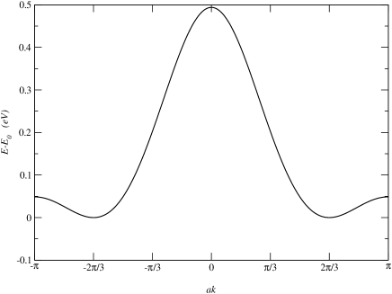
Figure 2: Effective holes lowest-band emerging from our theory. Parameters are $t=0.24,J_{K}=1$ eV.The minimum falls exactly at $(ak)=2\pi/3$

Now that we calculated the long wavelength contribution coming from the holes, we still have to consider the continuum limit (in the low energy sector) of the pure spin action $S_{s}$ given by eq. (6). The result is

$$S_{s\textrm{ eff}} = -i\int\!dx\,d\tau\left(\mathbf{N}\times\partial_{\tau}\mathbf{N}\right)\cdot\left(\mathbf{l}_{1}+\mathbf{l}_{2}\right)+a\left(J_{\|}+\frac{J_{\perp}}{2}\right)\int\!dx\,d\tau\left(\mathbf{l}_{1}+\mathbf{l}_{2}\right)^{2}$$ (38)

$$+aJ_{\|}\int\!dx\,d\tau\left(\mathbf{l}_{1}-\mathbf{l}_{2}\right)^{2}+aS^{2}J_{\|}\int dx\,d\tau\,\left|\partial_{x}\mathbf{N}\right|^{2}.$$

The very last step is the Gaussian integration of the $\mathbf{l}_{\perp}$ field, leaving us with the effective long-wavelength action for the antiferromagnetic order parameter, a (1+1) NL$\sigma$M:

$$S_{\textrm{eff}}=S_{h\textrm{ eff}}+S_{s\textrm{ eff}}=\frac{1}{2f}\int dxd\tau\left[v\left|\partial_{x}\mathbf{N}\right|^{2}+\frac{1}{v}\left|\partial_{\tau}\mathbf{N}\right|^{2}\right],$$ (39)

where the NL$\sigma$M parameters are given by

$$f = \frac{1}{2}\left[\left(S^{2}J_{\|}-\frac{\bar{\chi}_{xx}}{2}\right)\left(\frac{\left(1+\frac{g^{3}}{S}\hat{\chi}_{\tau}\right)^{2}}{\left[4J_{||}+2J_{\perp}+\frac{g^{2}}{S^{2}}\tilde{\chi}\right]}-\frac{\bar{\chi}_{\tau\tau}}{2}\right)\right]^{-\frac{1}{2}},$$ (40)

$$v = a\left[\frac{\left(S^{2}J_{\|}-\frac{\bar{\chi}_{xx}}{2}\right)}{\left(\frac{\left(1+\frac{g^{3}}{S}\hat{\chi}_{\tau}\right)^{2}}{\left[4J_{||}+2J_{\perp}+\frac{g^{2}}{S^{2}}\tilde{\chi}\right]}-\frac{\bar{\chi}_{\tau\tau}}{2}\right)}\right]^{\frac{1}{2}}.$$ (41)

Hence, the spin-fermion model with mobile holes interacting with an antiferromagnetic background is mapped into an effective NL$\sigma$M whose coupling constant depend on doping through the generalized susceptibilities in Eqs. (34), (36), and (37).

Now we can immediately transpose to our model of a doped spin liquid, some known result for the NL$\sigma$M, e. g. mainly the presence of a gap which separates the singlet ground state from a triplet of magnetic excitations. This gap should persist as long as the continuum approximation is valid.

The fact that the NL$\sigma$M in (1+1) dimension has a gap above the ground state can be established in a variety of ways. Using the two loop beta function Brezin and Zinn-Justin (1976) one obtains

$$\Delta=v\Lambda e^{-\frac{2\pi}{f}}\left(\frac{2\pi}{f}+1\right),$$ (42)

where $\Lambda$ is a cutoff of the order of the inverse lattice constant. Now we have an explicit analytic form for the doping dependence of the spin gap in the spin-liquid state of a two leg ladder.

To study the behavior of the gap with doping we have to distinguish two regimes where the lowest effective band has minimum either at zero or at $2/3\pi$. For $J_{K}>2t$ the minima fall in $\pm 2/3\pi$. Here all the generalized susceptibilities in Eqs. (34), (36), and (37) contribute to lower $f$ and, since from eq. (42) $\Delta$ is an increasing function of $f$, they make the gap smaller for any value of the constants (see Fig. 3). This is comforting, since, as we mentioned, for $J_{K}$ very large the physics of the Spin-Fermion model should be similar to that of the $t-J$ model Zhang and Rice (1988), and for that one, TDMRG simulations show that the gap decreases at least in a strong anisotropic case ($J_{\perp}=10J_{\|}$). When $J_{K}<2t$ the band minimum falls in zero and there is one susceptibility, $\tilde{\chi}$, which instead makes $f$ grow. $f$. In this regime there is then a (small) region of parameters where the gap grows with doping (see figure 4).

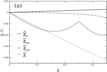
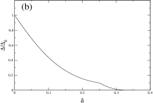
Figure 3: $J_{K}>2t$. (a) Generalized susceptibilities of Eqs. (34), (36), and (37) for $J_{K}=2,\,t=0.76$ eV. For $J_{K}>2t$ all the susceptibilities contribute to lower $f$ hence the gap decreases for small doping for any value of the constants. (b) Normalized gap of eq. (42). Here we fixed the exchange constants to $J_{\parallel}=J_{\perp}=0.108$ eV. $\Delta_{0}$ is the gap without doping.

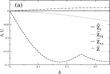
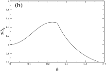
Figure 4: $J_{K}<2t$. (a) Generalized susceptibilities of Eqs. (34), (36), and (37) for $J_{K}=3\,t=1.8$ eV. For $J_{K}<2t$, one susceptibility, $\tilde{\chi}$, grows with doping and contributes to increase $f$ and hence the gap. For $(J_{K},t)\gg(J_{\parallel},J_{\perp})$ we can have an increasing gap for small doping. (b) Normalized gap of eq. (42). Fixing the exchange constants to $J_{\parallel}=J_{\perp}=0.108$ eV is enough to have an increasing gap for small doping.

Before passing to a comparison with experiments, we want to comment on a possible simplifying understanding.

A simple picture to explain the observed diminishing of the spin gap with doping in $\textrm{Sr}_{14-x}\textrm{Ca}_{x}\textrm{Cu}_{24}\textrm{O}_{41}$, is that (at least for low doping concentration where speaking of a spin liquid is still feasible) the effect of the holes is that of renormalizing the anisotropy parameter $\lambda=J_{\perp}/J_{\|}$ for the spin part towards larger values. In many studies on the 2 leg ladder Heisenberg antiferromagnet Gopalan et al. (1994); Reigrotzki et al. (1994); Greven et al. (1996), the spin gap is seen to increase with $\lambda$. In fact, the same occurs in the NL$\sigma$M without doping in the range $\lambda\approx 1\div 2$.

We can now pass to our mapping of a doping spin liquid to an effective NL$\sigma$M. According to equations (40,41) effective coupling constants $\tilde{J}_{\|},\tilde{J}_{\perp}$ can be defined for the doped system such that the form of the NL$\sigma$M parameters is that for a pure spin system Dell’Aringa et al. (1997) i. e.

$$f = \frac{1}{S}\sqrt{1+\frac{\tilde{J}_{\perp}}{2\tilde{J}_{\|}}},$$ (43)

$$v = 2aS\tilde{J}_{\|}\sqrt{1+\frac{\tilde{J}_{\perp}}{2\tilde{J}_{\|}}}.$$ (44)

A small doping expansion in the regime $J_{K}>2t$ leads to

$$\tilde{J}_{||} = J_{||}+\frac{3}{4}\frac{\left(J^{2}_{K}-4t^{2}\right)}{J_{K}}\delta+O\left(\delta^{2}\right),$$ (45)

$$\tilde{J}_{\perp} = J_{\perp}-\left(\frac{3}{2}\frac{\left(J^{2}_{K}-4t^{2}\right)}{J_{K}}+2\left(4J_{||}+2J_{\perp}\right)+\frac{\left(4J_{||}+2J_{\perp}\right)^{2}}{8J_{K}}\right)\delta+O\left(\delta^{2}\right),$$ (46)

so indeed $\tilde{J}_{\|}$, $\tilde{J}_{\perp}$ are seen respectively to increase, decrease, such that $\lambda$ decreases. However, such an interpretation breaks down beyond $\delta\approx 0.04$ whereas $f,v$ are still well defined positive constants. This means that beyond such doping, this simplified picture cannot be naïvely applied and holes have a more effective way of lowering the gap.

III Comparison with Experiments

We come now to the comparison with experiments. Our theory depends on four parameters $t,J_{K},J_{\parallel},J_{\perp}$ which we now want to fix to physical values. ARPES experiment on $\textrm{Sr}_{14}\textrm{Cu}_{24}\textrm{O}_{41}$ were performed by Takahashi et. al.  Takahashi et al. (1997) who found a band matching the periodicity of the ladder with a bandwidth of $\sim 0.5\div 0.4$ eV. Adjusting our lowest band to have such a bandwidth we obtain a relation between $t$ and $J_{K}$. On the other hand, experiments on the CuO₂ cell materials and band theory calculation Nücker et al. (1988); Singh et al. (1989); Hybersten et al. (1989) agreed in assuming a value of $J_{K}$ of the order of $J_{K}\approx 1\div 2$ eV. This in turn gives us a value of $t\approx 0.24\div 0.76$ eV, which is also consistent with the same calculation.

The debate around an anisotropy of the spin exchange constants Eccleston et al. (1998); Katano et al. (1999) in $\textrm{Sr}_{14-x}\textrm{Ca}_{x}\textrm{Cu}_{24}\textrm{O}_{41}$ seems now to be resolved in favor of isotropy or light anisotropy of the coupling constant: $J_{\perp}/J_{||}\approx 0.8$ Gozar et al. (2001). We adjusted the value of the momentum cutoff $\Lambda$ by fixing the theoretical gap with the experimental one for the undoped compound $\textrm{Sr}_{14}\textrm{Cu}_{24}\textrm{O}_{41}$. Finally, to compare with the measured values of the gap for different doping concentration $x$ in $\textrm{Sr}_{14-x}\textrm{A}_{x}\textrm{Cu}_{24}\textrm{O}_{41}$ (where $A$ can be either divalent $\textrm{Ca}^{2+},\textrm{Ba}^{2+}$ or trivalent $\textrm{Y}^{3+},\textrm{La}^{3+}$), we still need a relation between the A substitution $x$ and the number of holes per copper site present in the ladder $\delta$. This is another unsettled issue of the telephone number compound. In particular Osafune et. al.  Osafune et al. (1997) studying the optical conductivity spectrum, inferred that with increasing Ca substitution $x$, holes are transferred from the chain to the ladder. On the other hand Nücker et. al.  Nücker et al. (2000) argue that in the series compound $\textrm{Sr}_{14-x}\textrm{Ca}_{x}\textrm{Cu}_{24}\textrm{O}_{41}$ the number of holes in the ladder is almost insensitive to Ca substitution $x$ (although a small increase is observed). Here we will assume that $\textrm{Sr}_{14-x}\textrm{A}_{x}\textrm{Cu}_{24}\textrm{O}_{41}$ is an example of doped spin liquid and will use the data from Osafune et al. (1997). The result of our theory can be seen in figure 5. There we used isotropic exchange constant, but the theoretical curve did not change in a visible way if an anisotropy of $J_{\perp}/J_{||}\approx 0.8$ was inserted. We see from the figure that the spin gap becomes zero for $\delta\approx 0.37$, beyond this value the coupling constants $f$ and $v$ would become imaginary signaling that our effective model cease to make sense. This means that for such doping ratios our parameterization (15) is no longer valid, in the sense that it does not incorporate the most important spin configurations. However our theory could cease to make sense much before. If one takes the point of view of the $t-J$ model (as we said the Spin-Fermion model should map to it for large $J_{K}$) the holes introduced in the system couple rigidly to the spins forming singlet with the $P_{i}$ states. In the worst case this would limit the correlation length of the spin to the mean hole-hole distance $1/\delta$. In our case this happens at a doping ratio of $\delta\approx 0.15$.

A word of caution should be mentioned with respect to comparison with experimental results. A still unresolved controversy is present between NMR Kumagai et al. (1997); Magishi et al. (1988); Carretta et al. (1998) and neutron scattering Eccleston et al. (1998); Katano et al. (1999) experiments, where the latter see essentially no doping dependence of the spin gap. Without being able to resolve this issue, we would like, however, to stress, that beyond the uncertainties in experiments, the doping behavior obtained for the spin-gap agrees with the numerical results in TDMRG and is opposite to the one obtained in mean-field treatments, making clear the relevance of fluctuations.

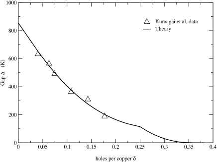
Figure 5: Result of our theory and comparison with experiments. The values of the constants used in equation (42) are $t=0.76,J_{K}=2$ eV, $J_{\parallel}/J_{\perp}=1$. The momentum cutoff $\Lambda$ was fixed by fixing the the value of the gap with the one measured in $\textrm{Sr}_{14}\textrm{Cu}_{24}\textrm{O}_{41}$. For anisotropic case $J_{\perp}/J_{\parallel}=0.8$ the curve does not change appreciably.

IV Conclusion

In this paper we studied the behavior of the spin gap of a two leg Heisenberg antiferromagnetic ladder as microscopically many holes are introduced in the system. Such a situation can be physically realized in the series compound $\textrm{Sr}_{14-x}\textrm{A}_{x}\textrm{Cu}_{24}\textrm{O}_{41}$ with A=Ca, Y, La, and numerous result are now available from experiments. On the theoretical side, however, there is a contradiction between previous analytical treatments on the one hand, and TDMRG simulations or NMR experiments on the other hand. Whereas in the first case, a magnon gap increasing with doping is predicted, a decrease is observed in accurate numerical simulation and experiments.

Starting from the spin-fermion model we were able to solve the contradiction using a controlled analytical treatment that properly takes into account fluctuations in the continuum limit. Integrating out the fermions we were left with a Fermi-determinant which we can evaluate exactly in that limit. The result is a non linear $\sigma$ model with doping dependent parameters. The spontaneously generated mass gap of this theory is seen to decrease as holes are introduced. Once physical value for the parameters are given, we obtained very good agreement with NMR experiments performed on Sr_14-xA_xCu₂₄O₄₁.