Scattering of atoms on a Bose–Einstein condensate

Abstract

We study the scattering properties of a Bose–Einstein condensate held in a finite depth well when the incoming particles are identical to the ones in the condensate. We calculate phase shifts and corresponding transmission and reflection coefficients, and we show that the transmission times can be negative, i.e., the atomic wavepacket seemingly leaves the condensate before it arrives.

I Introduction

In this paper we present an analysis of the scattering of atoms on a Bose-Einstein condensate. A repulsive interaction between atoms is both responsible for the shape of the condensate and for the interaction between the incident atom and the condensed atoms. Scattering effects can be significant when two condensates merge, and four-wave mixing has been observed in experiments Deng et al. (1999). We deal here with the limit of a single or just a few atoms, incident in a well defined momentum state on a condensate, a situation that has been realized experimentally to seed atom lasers Vogels et al. (2002) and ’atomic parametric amplifiers’ Inouye et al. (1999, 2000) with a weak atomic beam. Our interest, however, is in the interaction between the small atomic component and the condensate, and in particular in the transmission and reflection properties of the condensate as a beam splitter for atoms of the same kind as the mirror itself. Since the atoms of the scatterer are indistinguishable from the scattered particles, exchange effects play an important role, and similar scattering studies have indeed been proposed as a means for investigating superfluidity in strongly interacting He-4 system Halley et al. (1993); Setty et al. (1997), and also in weakly interacting systems Wynveen et al. (2000).

Dilute condensates can be trapped in a large number of trapping arrangements, and we shall assume a trapping potential of finite width allowing asymptotically free atoms to be directed towards the trapped condensate and interact with it in a well defined region of space. Such potentials can be created optically or possibly in the region above a current carrying chip, and our calculations, which will be carried out in a one dimensional geometry, may correspond to either a condensate slab hit by atoms with well defined transverse momenta or to a trapped condensate in a wave guide with a local longitudinal minimum.

In Sec. II we introduce the Bogoliubov treatment of excitations of a Bose-Einstein condensate. In Sec. III we explain how an analysis of the fundamental excitations of the condensate provides the scattering information. Numerical results are compared with an approximate analytical model. In Sec. IV, we show examples of time dependent wavepacket dynamics, and we identify a momentum regime in which transmission occurs with negative time delays, i.e., the wave packet emerges from the condensate before it arrives. Sec. V concludes the paper.

II The Bogoliubov Approach

In the Bogoliubov approach, the number of particles in the condensate mode is assumed to be high and rather well defined, and the problem of small thermal or externally induced excitations can be treated to lowest order to yield a picture of non-interacting quasi-particles. These are the normal modes of the system and they are mixtures of particle- and hole-like excitations. In the case of scattering, the incoming particle will behave as a quasiparticle while moving through the condensate, whereas asymptotically the excitation is particle-like as hole-excitations are limited to the region occupied by the condensate.

Let us briefly review the Bogoliubov approach. First, the field operator is written in a form explicitly emphasizing the condensate mode

$$\hat{\Psi}(x)=\sqrt{N}\phi_{0}(x)+\delta\hat{\Psi}(x).$$ (1)

Here $\phi_{0}(x)$ is to be regarded as a $c$-number field describing the condensate while $\delta\hat{\Psi}(x)$ describes the correction. We insert this form in the full Hamiltonian (in the contact–interaction approximation),

$$\hat{H}=\int\!dx\;\biggl{\{}\hat{\Psi}^{\dagger}(x)h(x)\hat{\Psi}(x)\\ +\frac{g_{\text{1D}}}{2}\hat{\Psi}^{\dagger}(x)\hat{\Psi}^{\dagger}(x)\hat{\Psi}(x)\hat{\Psi}(x)\biggr{\}},$$ (2)

where $h(x)=-(\hbar^{2}/2m)\partial_{x}^{2}+V(x)$ is the single-particle Hamiltonian and $g_{\text{1D}}$ quantifies the 1D interaction strength. Keeping only interaction terms of order $N$ or higher, we arrive at a quadratic form in $\delta\hat{\Psi}(x)$ and $\delta\hat{\Psi}^{\dagger}(x)$. The terms linear in $\hat{\Psi}(x)$ and $\hat{\Psi}^{\dagger}(x)$ are identically zero if $\phi_{0}(x)$ solves the Gross–Pitaevskii equation

$$\left[h(x)+gN|\phi_{0}(x)|^{2}\right]\phi_{0}(x)=\mu\phi_{0}(x).$$ (3)

To diagonalize the remaining part, one envokes a Bogoliubov transformation and writes

$$\delta\hat{\Psi}(x)=\sum_{k}\left[\hat{b}_{k}u_{k}(x)-\hat{b}^{\dagger}_{k}v_{k}^{*}(x)\right],$$ (4)

where $u_{k}(x)$ and $v_{k}(x)$ solve the Bogoliubov–de Gennes equations:

$$[L(x)-\hbar\omega_{k}]u_{k}(x) =gn_{0}(x)v_{k}(x)$$ (5)

$$[L(x)+\hbar\omega_{k}]v_{k}(x) =gn_{0}(x)u_{k}(x)$$ (6)

and are normalized to

$$\int\left[u_{k}^{*}(x)u_{k^{\prime}}(x)-v_{k}^{*}(x)v_{k^{\prime}}(x)\right]dx=\delta_{kk^{\prime}}.$$ (7)

The operator $L(x)$ is defined by $L(x)=h(x)+2gn_{0}(x)-\mu$. The Hamiltonian finally takes the simple form

$$\hat{H}_{\text{diag}}=E(N)+\sum_{k=1}^{\infty}\hbar\omega_{k}\hat{b}^{\dagger}_{k}\hat{b}_{k},$$ (8)

i.e, it describes non-interacting quasi–particles created by $\hat{b}^{\dagger}_{k}$ and destroyed by $\hat{b}_{k}$. Note how the Bogoliubov transform mixes creation and destruction operators. This means, that excitations have both a particle–like character (described by $u_{k}$) and a hole–like character (describe by $v_{k}$).

The Bogoliubov analysis is routinely applied to the case of a homogeneous situation (flat potential) and the case of an infinite trapping potential Dalfovo et al. (1999). In the first case, one obtains solutions with well–defined momenta: phonons in the long wave–length limit, free particles for high momenta. The spectrum is continuous and gap–less. In the second case, the excitations are again collective in the low energy regime, approaching single–particle trap states for high energies Öhberg et al. (1997). The spectrum is discrete. Here we will concentrate on a third situation where the trapping potential has finite width and depth. In this scenario, a finite number of trapped excitations exists and above these a continuum of scattering states. The corresponding spherically symmetric problem in 3D has been treated by Wynveen et al. in Wynveen et al. (2000).

Away from the trap and thus from the condensate, the scattering states are particle–like ($v_{k}(x)=0$) and the usual asymptotic analysis of scattering applies: We can define incoming, reflected, and transmitted fluxes and we can set up an initial wave–packet and make it progate towards the condensate region. The actual tranmission and reflection coefficients depend on what happens while the incoming particle passes through the condensate and this propagation is partly phonon–like, i.e., with the emergence of a hole–like component.

In 1D, the Bogoliubov–De Gennes equations are computationally quite manageable and the choice of method for their solution is not crucial. Nevertheless, for completeness we here briefly summarize our method. First we solve the Gross–Pitaevskii equation (3) with the chosen potential. We do this by a simple steepest descent method, i.e., by propagating the corresponding time–dependent equation in imaginary time. In particular, we use a split–step fast–Fourier–transform algoritm Fleck et al. (1976). In Fig. 1, we show the particular potential we will be using, and we show the corresponding condensate wavefunction.

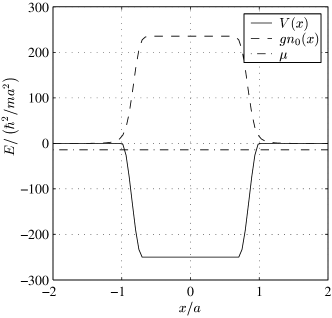
Figure 1: Figure showing the potential well and the shape of the condenste. The range of the potential is $[-a,a]$ outside which $V(x)$ is identically 0. $V(x)$ changes smoothly to $-V_{0}=-250\hbar^{2}/ma^{2}$ in edge–zones of width $0.3a$. The 1D interaction strength is taken to be $g_{\text{1D}}N=400\hbar^{2}/ma$. The solution of the GPE (3) then gives $\mu=-14.4\hbar^{2}/ma^{2}$ and a Bogoliubov speed of sound $c=\sqrt{gn_{0}(0)/m}=15.4\hbar/ma$ in the inner region of the well.

When $\phi_{0}(x)$ and $\mu$ have been found, Eqs. (5) and (6) are solved by first defining

$$\begin{split}f_{k}(x)&=\sqrt{\frac{1}{2}}\left[u_{k}(x)+v_{k}(x)\right]\\ h_{k}(x)&=\sqrt{\frac{1}{2}}\left[u_{k}(x)-v_{k}(x)\right]\end{split}$$ (9)

in terms of which Eqs. (5) and (6) become

$$[L(x)-gn_{0}(x)]f_{k}(x) ={\hbar\omega_{k}}h_{k}(x)$$ (10)

$$[L(x)+gn_{0}(x)]h_{k}(x) =\hbar\omega_{k}f_{k}(x)$$ (11)

We can then avoid diagonalizing a two–component problem by simply applying the operator $[L(x)+gn_{0}(x)]$ to both sides of Eq. (10) to find the necessary condition

$$[L(x)+gn_{0}(x)][L(x)-gn_{0}(x)]f_{k}(x)=[\hbar\omega_{k}]^{2}f_{k}(x).$$ (12)

When this one–component eigenvalue problem is solved, $u_{k}(x)$ and $v_{k}(x)$ can be found by applying first Eq. (10) and then Eq. (9).

III Results

III.1 Phaseshifts

We assume that $V(x)$ and thus $n_{0}(x)$ have even spatial symmetry. We can then demand that solutions of Eqs. (5) and (6) have definite parity. In the discrete part of the spectrum, even and odd solutions alternate, while in the continuum, each energy supports solutions of both parities. In the asymptotic region away from the potential and the condensate, even and odd scattering solutions can then be written

$$\begin{array}[c]{lcl}u^{(e)}_{k}(x)&\rightarrow&\cos(kx\mp\delta_{e}(k))\\ u^{(o)}_{k}(x)&\rightarrow&\sin(kx\mp\delta_{o}(k))\end{array}\quad\text{for\ }x\rightarrow\pm\infty.$$ (13)

Note that we identify the label $k$ with the asymptotic wavenumber for the scattering solutions. The phaseshifts, $\delta_{e}(k)$ and $\delta_{o}(k)$, contain all the information about the scattering relevant to the asymptotic region. They can be conveniently extracted from our numerical solutions for $u_{k}$. The calculations are actually done on a space–interval $[-L,L]$ with periodic boundary conditions (finite lower momentum cutoff). This means that for a given $L$ we only find the subset of the continuum solutions with wavenumbers fulfilling

$$-kL+\delta(k)\equiv kL-\delta(k)\mod 2\pi$$ (14)

or, equivalently,

$$\delta(k)\equiv kL\mod\pi.$$ (15)

After the diagonalization this discrete set of $k$ values can easily be determined from the eigenvalues as $\hbar\omega_{k}=\hbar^{2}k^{2}/2m-\mu$. Each $k$ value gives us one point on $\delta(k)$ via Eq. (15). This is enough to determine $\delta(k)$ if it is slowly varying on the $1/L$ scale. If not, we just need to change $L$ slightly and repeat the calculation to obtain an additional set of points.

In Fig. 2

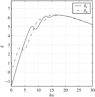
Figure 2: Phaseshifts of even and odd solutions as a function of incoming momentum. Parameters as in Fig. 1.

we show a typical example of $\delta_{e}(k)$ and $\delta_{o}(k)$ with parameters as in Fig. 1. There is clearly some resonant behavior with out–of–phase oscillations of $\delta_{e}(k)$ and $\delta_{o}(k)$ around a slowly varying average. This behaviour is well known from ordinary, single particle scattering on a well/barrier, and in the following subsection we shall present an analytical model which yields the same gross features.

III.2 Square well model, Thomas–Fermi approximation

Let us consider a condensate trapped in a square well potential

$$V(x)=\left\{\begin{array}[c]{lcl}-V_{0}&,&|x|<a_{\text{sw}}\\ 0&,&|x|>a_{\text{sw}}\\ \end{array}\right.$$ (16)

where $a_{\text{sw}}$ is an appropriately defined effective width. In the Thomas–Fermi approximation the condensate wave function is constant in the trap and zero outside

$$\phi_{0}(x)=\left\{\begin{array}[c]{lcl}\sqrt{\frac{N}{2a_{\text{sw}}}}&,&|x|<a_{\text{sw}}\\ 0&,&|x|>a_{\text{sw}}\\ \end{array}\right..$$ (17)

This $\phi_{0}(x)$ is naturally not a solution to the Gross–Pitaevskii equation as the kinetic energy term will smoothen the step in density even when the external potential is discontinuous. Formally, this introduces linear terms in Eq. (8), i.e., the Bogoliubov vacuum is not a steady–state for the system. We are, however, only interested in the scattering behaviour at positive energies and it is reasonable to assume that some insight can be gained by finding solutions to Eqs. (5) and (6) with the simplifying assumptions expressed by (16) and (17).

It is amusing to note, that we are now dealing with the Bogoliubov–de Gennes analog of the undergraduate textbook problem of 1D scattering on a square well. The full solution is found by matching the analytical wavefunctions in the regions, $x\in[-\infty,-a_{\text{SW}}]$, $[-a_{\text{SW}},a_{\text{SW}}]$, and $[a_{\text{SW}},\infty]$. To the left and to the right of the well, we demand $v(x)=0$ and let $u(x)=\cos(kx\pm\delta_{e}(k))$ ($u(x)=\sin(kx\pm\delta_{o}(k))$) to find even (odd) solutions. Inside the well, we are in a region of constant potential ($V(x)=-V_{0}$) and constant condensate density ($N|\phi_{0}(x)|^{2}=n_{0}$) so Eqs. (5) and (6) read

$$\left[-\frac{\hbar^{2}}{2m}\partial_{x}^{2}-V_{0}+2gn_{0}-\mu-\hbar\omega\right]u(x) =gn_{0}v(x)$$ (18)

$$\left[-\frac{\hbar^{2}}{2m}\partial_{x}^{2}-V_{0}+2gn_{0}-\mu+\hbar\omega\right]v(x) =gn_{0}u(x).$$ (19)

To be able to match the boundary conditions, we need four linearly independent solutions and the ansatz $u(x)=Ue^{i\lambda x}$, $v(x)=Ve^{i\lambda x}$ leads to $\lambda\in\{\pm\lambda,\pm\tilde{\lambda}\}$ where

$$\hbar\lambda(k)=\\ \sqrt{2m\left(\sqrt{\left[gn_{0}\right]^{2}+\left[E-\mu\right]^{2}}-2gn_{0}+V_{0}+\mu\right)}$$ (20)

and

$$\hbar\tilde{\lambda}(k)=\\ i\sqrt{2m\left(\sqrt{\left[gn_{0}\right]^{2}+\left[E-\mu\right]^{2}}+2gn_{0}-V_{0}-\mu\right)}$$ (21)

where $E=(\hbar k)^{2}/2m$ is the incoming kinetic energy. Note that $\tilde{\lambda}$ is imaginary and it is normally disregarded in homogeneous condensates. Here, it is needed as we must match the boundary conditions that also $v$ and $v^{\prime}$ are continuous.

The matching of $u$ and $v$ at $x=a_{\text{sw}}$ leads to equations for the phaseshifts. They read

$$\tan\left(ka_{\text{sw}}-\delta_{e}(k)\right) = \frac{\lambda(k)}{k}\tan\left(\lambda(k)a_{\text{sw}}\right)$$ (22)

$$\tan\left(ka_{\text{sw}}-\delta_{o}(k)\right) = \frac{k}{\lambda(k)}\tan\left(\lambda(k)a_{\text{sw}}\right).$$ (23)

These equations are the same as for single particle square well scattering except that the usual $\hbar\lambda=\sqrt{2m(E-V)}$ is replaced by $\hbar\lambda$ from Eq. (20).

In Fig. 3 we show results obtained for parameters like in Fig. 1: $gn_{0}$ is taken as the central density in the smooth trap and $a_{\text{sw}}$ is chosen to accomodate the same total number of particles. A comparison with Fig. 2 reveals both similarities and differences: The smooth behaviour of the average of the two curves is well reproduced as well as the (quasi–)period of the oscillatory behaviour. However, the positions of curve crossings and the maxima of the phaseshift differences, especially at low $k$’s, are not well reproduced. Also, at high momenta the sharp–edge approximation leads to stronger oscillations in $\delta_{e}(k)$ and $\delta_{o}(k)$ than for the smooth well.

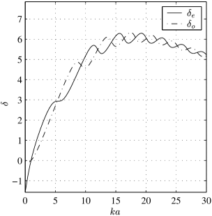
Figure 3: Even and odd phaseshifts for a simple square well/square condensate model. The parameters are like in Fig. 1 and the curves should be compared to the full numerical calculations presented in Fig. 2. There is clearly a qualitative agreement: The smooth behavior of the average of the two curves is well reproduced and the periode of the oscillations around this average is also of the correct order of magnitude. However, the oscillations extend to too high values of $k$.

III.3 Transmission coefficent

The typical scattering situation with an incoming, a reflected, and a transmitted wave specifies the asymptotic form of the wave function

$$u_{k}(x)\rightarrow\left\{\begin{array}[c]{lcl}e^{ikx}+R(k)e^{-ikx}&\text{for}&x\rightarrow-\infty\\ T(k)e^{ikx}&\text{for}&x\rightarrow\infty\end{array}\right..$$ (24)

This defines the reflection- and transmission-coefficients $R(k)$ and $T(k)$. Making the change of basis from the odd and even parity eigenstates (13), one finds

$$\begin{split}R(k)&=\frac{1}{2}\left(e^{-2i\delta_{e}(k)}-e^{-2i\delta_{o}(k)}\right)\\ &=ie^{-i(\delta_{o}(k)+\delta_{e}(k))}\sin(\delta_{o}(k)-\delta_{e}(k))\end{split}$$ (25)

$$\begin{split}T(k)&=\frac{1}{2}\left(e^{-2i\delta_{e}(k)}+e^{-2i\delta_{o}(k)}\right)\\ &=e^{-i(\delta_{o}(k)+\delta_{e}(k))}\cos(\delta_{o}(k)-\delta_{e}(k)).\end{split}$$ (26)

We see that 100% transmission takes place at $k$’s where $\delta_{e}(k)=\delta_{o}(k)$ while 100% reflection requires $\delta_{e}(k)=\delta_{o}(k)\pm\pi/2$. In Fig. 4 we plot $R$ and $T$ for the same situation as considered above. The curve crossings in Fig. 2 are now translated into transmission windows. At very low momenta, we get 100% reflection and at very high momenta we naturally get 100% transmission.

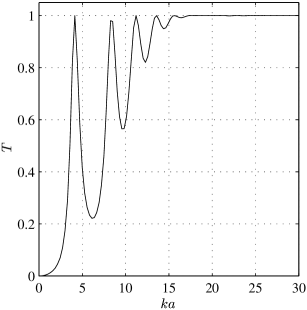
Figure 4: Transmission and reflection coefficients for the situation considered in Figs. 1 and 2. A series of perfect transmissions are seen, corresponding to the crossings of the $\delta_{e}(k)$ and $\delta_{o}(k)$ curves in Fig. 2.

IV Time dependent scattering

IV.1 Wavepacket dynamics

With the complete set of scattering states it is possible to follow scattering of wavepackets in time. To obtain the initial state we add a number of particles to the Bogoliubov vacuum:

$$|t=0\rangle=\frac{1}{\sqrt{n_{s}!}}\left[\int\phi_{\text{s}}(x)\delta\hat{\Psi}^{\dagger}(x)\right]^{n_{s}}|\text{vac}\rangle$$ (27)

where $\phi_{\text{s}}(x)$ is the desired wavepacket mode. The operator term in this equation creates an $n_{s}$–particle state, but to benefit from the simple form of Eq. (8) we should think of it as creating $n_{s}$ quasiparticles which at $t=0$ just happen to be localized well away from the condensate. The quasiparticles are created in a superposition of energy eigenstates and the coefficients in this superposition are found as

$$c_{k}=\int\left[u_{k}^{*}(x)\phi_{\text{s}}(x)+v_{k}^{*}(x)\phi_{\text{s}}^{*}(x)\right]dx.$$ (28)

As $\phi_{s}$ is located well away from the condensate region, there is in fact no contribution from the $v$ part of this integral.

The time evolution is entirely given by the relation $\hat{b}_{k}(t)=e^{-i\omega_{k}t}\hat{b}_{k}$ in the Heisenberg picture, and we find the non–condensate mode part of the total density to be

$$\langle\delta\hat{\Psi}^{\dagger}(x)\delta\hat{\Psi}(x)\rangle=n_{s}\left|U(x,t)\right|^{2}+n_{s}\left|V(x,t)\right|^{2}+\sum_{k}\left|v_{k}(x)\right|^{2}$$ (29)

where

$$U(x,t) =\sum_{k}c_{k}e^{-i\omega_{k}t}u_{k}(x)$$ (30)

$$V(x,t) =\sum_{k}c_{k}e^{-i\omega_{k}t}v_{k}(x).$$ (31)

The last term in Eq. (29) is the quantum depletion, which is always present due to the interactions in the condensate, while the first two terms are consequences of the scattering process.

Depending on the spread of $k$-values in the wavepacket, the asymptotic behaviour of the scattering will be more or less simply described by reading off the reflection and transmission coefficients $R$ and $T$ at the average momentum $k_{0}$. In fact, looking at the first form of these coefficients in Eqs. (25) and (26) we are reminded that the reflected and the transmitted wave can be seen as superpositions of an even part and an odd part. To each of these can be ascribed a time-delay, $\Delta t_{e/o}$ in the arrival of the original wave packet at certain point in space with respect to the free propagation. It is easy to show that these delays are given by

$$\Delta t_{e} = \left.-\frac{2}{v_{g}}\frac{\partial\delta_{e}(k)}{\partial k}\right|_{k=k_{0}}$$ (32)

$$\Delta t_{o} = \left.-\frac{2}{v_{g}}\frac{\partial\delta_{o}(k)}{\partial k}\right|_{k=k_{0}}$$ (33)

where $v_{g}=\hbar k_{0}/m$ is the (group) velocity of the incoming wavepacket. If these delays are sufficiently different the reflected and transmitted wavepackets are expected to be doublepeaked. In fact, a closer look at Eqs. (25) and (33) reveals a difference in sign: the reflected wavepacket can easily be double–peaked as it is the difference between the even and odd contribution, while the transmitted wavepacket is the sum and therefore require displacements as large as the wavepacket width for a visible effect.

In Fig. 5 we show time series of snapshots from wavepacket simulations. The double peak phenomenon mentioned above is visible in the $k_{0}a=11.20$ timeserie. This $k_{0}$ corresponds to a crossing of $\delta_{e}(k)$ and $\delta_{o}(k)$ and thus to both high tranmission and a marked difference in $\Delta t_{e}$ and $\Delta t_{o}$ (cf. Fig. 2).

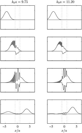
Figure 5: Wavepacket scattering on a BEC. Time series are shown for two different incoming momenta: At mean wavenumber $k_{0}a=9.75$, the initial packet propagates towards the potential well containing the BEC and reflected and transmitted wavepackets appear. In accordance with Fig. 4 transmission is approximately 62% at this $k_{0}$. At $k_{0}a=11.2$ we are in a transmission window and the reflected wavepacket has small amplitude and a double–peaked envelope.The figures show both $|U(x)|^{2}$ and $-|V(x)|^{2}$, the particle contribution and ($-$) the hole contribution to the total density of scattering atoms. Note that the ground state quantum depletion also contributes to the density of atoms out of the condensate mode. This contribution is located inside the well and is not plotted here.

IV.2 Transmission times

The time–delays of Eqs. (32) and (33) can also be translated into an effective transmission time, the time spent traversing the condensate region. The well has a width $2a$ so the time spent inside the well can heuristicly be defined as $\tau=\Delta t+2a/v_{g}$. In Fig. 6 we plot $\tau_{e}(k)$ and $\tau_{o}(k)$. The two curves agree for high $k$, while for $ka$ less than $\sim 15$, i.e., for $v_{g}$ less than the Bogoliubov speed of sound in the homogeneous part of the condensate, $c=\sqrt{gn_{0}/m}$, they show alternating peaks. Such peaks are signatures of resonances where an even or an odd number of oscillations fit inside the condensate.

At low $k$–values, we observe that $\tau_{e}$ becomes negative over a rather wide range. For wavepackets with momentum components mainly in this range, a peak in the transmitted wavepacket can appear before the peak of the incident wavepacket has reached the condensate. This is confirmed by wavepacket simulations.

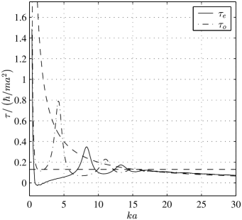
Figure 6: Time spent in the condensate region. Curves are shown for both even and odd solutions. Where these curves approximately coincide, the retardation can be seen directly in wavepacket scattering. When they are very different, the translation to a time–dependent wavepacket formulation is less direct. Note the negative values of $\tau_{e}$ in the region around $ka\lesssim 2$: Wavepacket simulations show that here the peak of the transmitted wavepacket appears before the peak of the incident wavepacket has reached the condensate. For comparison, the two dashed curves show respectively the free motion and the sound wave tranmission times, $2a/v_{g}$ and $2a/c$.

Negative transmission times is a wave phenomenon, which together with superluminal propagation has been observed for light propagation through wave guides and through dispersive atomic media. It is not suprising that the Bogoliubov-De Gennes equations show similar effects, and, indeed, Ray Chiao et al Chiao (to appear) have suggested a many-body interference mechanism that could lead to atomic transmission through condensates with negative transmission times. From our Bogoliubov analysis it is not clear if the result is due to this mechanism or if it is more closely related to the time delays, which may also be observed in normal wave packet tunneling through barriers Hartman (1962).

Note also that the analysis of both a real experiment and of wavepacket simulations is more complicated for massive particles than for light: As the transmission coefficient depends strongly on $k$, there is a velocity filter effect, i.e., the transmitted wavepacket may move at a different speed than the incoming one.

V Conclusion

It is well known that the Bogoliubov treatment leads to excited states ranging from phonon like disturbances of the mean field amplitude at low energies to particle like excitations at high enough energies. In the present case of a condensate trapped in a localized potential minimum of finite depth, the eigenspectrum of low energy excitations corresponds to states which are particle like in some regions of space and phonon like in others. Like in normal scattering theory, wave packets are formed as superpositions, and they propagate as a consenquence of the phase evolution of the energy eigenstates. In our study, this propagation implies that particles are incident on the condensate, they propagate as phonons through the condensate, where they may be reflected back and forth between the condensate edges, and eventually they reemerge as reflected or transmitted particles. We have determined the reflection and transmission probabilities and the phase shifts, which enable us to derive time dependent results from our stationary formulation. The main results of this analysis were double peaked distributions, reflected from the condensate and transmission with negative time delays. An experimental demonstration of the latter phenomenon would be an interesting supplement to similar studies for light transmission.

The particles are indistinguishable, and it is hence not meaningful to say that it is the same particle that emerges after the scattering process. The process, however, is coherent, and interferometric experiments should be able to show that coherence is maintained, just as experiments with quantum correlated atoms should reveal that also entanglement is faithfully preserved by the intermediate phonon excitation, in analogy with recent experiments where surface plasmons propagate quantum correlated photon pairs through sub wavelenght hole arrays Altewischer et al. (2002). We imagine that scattering experiments of the kind analyzed in this paper may be an ingredient in the study of controlled atomic dynamics, in particular for atoms and condensates trapped on chip architectures, Folman et al. (2000); Cassettari et al. (2000); Hänsel et al. (2001).