[

Quantum Dynamics in Non-equilibrium Strongly Correlated Environments

Abstract

We consider a quantum point contact between two Luttinger liquids coupled to a mechanical system (oscillator). For non-vanishing bias, we find an effective oscillator temperature that depends on the Luttinger parameter. A generalized fluctuation-dissipation relation connects the decoherence and dissipation of the oscillator to the current-voltage characteristics of the device. Via a spectral representation, this result is generalized to arbitrary leads in a weak tunneling regime.

] The quest to build a scalable quantum computer has recently lead to a series of spectacular experiments where macroscopic quantum states were coherently manipulated and measured[1, 2, 3]. These experiments for the first time give an opportunity to study the effects of indirect continuous measurement [4] on an individual quantum system. Understanding the measurement process is not only important for the development of a quantum computer, but also is a fundamental problem of quantum mechanics. In some cases, theoretical analysis of measurement process based on explicit models describing the coupling between the system and electrical measurement apparatus has been performed [5, 6, 7, 8, 9].

Correlations play a crucial role in protecting quantum coherence in macroscopic systems and enabling manipulation of the quantum states. In sub-micrometer electronic systems, the Coulomb interaction becomes important and can lead to Coulomb blockade, a subject of intensive research both in the contexts of “classical” and quantum-coherent electronic devices. The more subtle effects of itinerant electron-electron interactions, however, have not been studied in the context of quantum measurement. These effects are often important since in order to interface with a quantum device, at least a part of the apparatus has to be scaled down to the device size. The study of such correlation effects is therefore important in developing the understanding of a realistic quantum measurement.

To analyze the role of correlations in the measurement apparatus, we study here a specific example of two Luttinger liquid leads electrically coupled to a quantum system, with the tunneling current being influenced by a coordinate of the system. The Luttinger liquids are a generalization of the Fermi liquids to one dimension, where electron-electron interactions lead to dramatic renormalization effects near the Fermi surface[10]. The interactions in the Luttinger liquids can be parametrized by the dimensionless constant $g$, which describes repulsive interactions if $g<1$, attractive if $g>1$, and a non-interacting Fermi liquid for $g=1$. One experimental realization of Luttinger liquids is carbon nanotubes[11]. We develop the formalism for an arbitrary quantum system, which can be, for instance, a two-level system (qubit), or a quantum oscillator. For $g>1$, we find that the effect of the measurement is equivalent to coupling to a heat bath, with an effective temperature reduced relative to the Fermi liquid case[9]. The effective temperature depends on the density of states of the Luttinger liquids at the tunnel contact, $T_{\rm eff}=(\alpha+1)^{-1}qV/2$, where the current $I\propto V^{\alpha+1}$. The exponent $\alpha$ depends on the tunneling geometry and on the Luttinger parameter $g$. This provides an interesting example in which the Luttinger parameter determines, not an exponent, but a prefactor for a universal expression which is of first order in the bias voltage. It had been hoped that the two-terminal conductance of a one-dimensional wire would be proportional to $g$[12], providing another such example, but this turns out not to be the case[13]. Via a spectral representation, we find a relation valid for any leads in the weak tunneling regime with tunneling particles of charge $q$

$$T_{\rm eff}=(qI/2)({\rm d}V/{\rm d}I).$$ (1)

Examples of experimental realizations of our model as applied to the measurement of a quantum oscillator are shown in Fig. 1. In Fig. 1(a) and Fig. 1(b), the tunnel junction is formed by a nanotube (Luttinger liquid) and a metal (Fermi liquid), while in Fig. 1(c) and 1(d) both sides of the junction are Luttinger liquids. In the first example, Fig. 1(a), the tunnel current between the gate and the nanotube is used to monitor the transverse nanotube oscillations. The characteristic oscillation frequency is about 1 GHz for a 100 nm nanotube[14], which makes it possible to achieve the quantum regime at about 50 mK. In Fig. 1(b), a short stiff nanotube in the STM mode[15] is used to perform vibrational spectroscopy of an adsorbate loosely bound to a metal surface. The position of the atom/molecule modulates the tunnel current. In the last two examples a kink in the nanotube formed either mechanically or due to a 5-7 defect plays the role of the tunnel contact[11, 16]. The presence of the defect will lead to formation of a localized optical phonon mode above the nano-tube phonon band (above 200 meV[17]), that will couple to the tunnel current by modifying the tunneling matrix element. Alternatively, the chemical kink defect can be functionalized by adsorbing an atom or molecule[18], whose vibrations will also modify the tunneling between the two Luttinger legs.

Tunneling Between Two Luttinger Liquids— We consider the problem of tunneling between two Luttinger liquids, when the tunneling is coupled to an external system, such as a quantum oscillator, or a spin. The Hamiltonian is

$${\cal H}=\Omega T+{\cal H}^{L}_{1}+{\cal H}^{L}_{2}+{\cal H}_{0},$$ (2)

where ${\cal H}_{0}$ is the Hamiltonian for the measured system, referred to as an oscillator, ${\cal H}^{L}_{1,2}$ are the Luttinger liquid Hamiltonians for the two leads, with Luttinger parameter $g$ and with a potential difference $\mu=qV$. We define the electron tunneling operator $T(t)=\Psi^{\dagger}_{1}(x=0,t)\Psi_{2}(x=0,t)+h.c.$, where $\Psi_{1,2}(x,t)$ are fermion operators in the leads. The term $\Omega$ includes $c$-number terms as well as operators that do not commute with ${\cal H}_{0}$.

Following Kane and Fisher[16], we consider tunneling via a weak link, that is tunneling between two semi-infinite leads with $x=0$ located at the ends of the leads. We consider the case of repulsive interactions, $g<1$. For spinless fermions, the end density of states of a lead at energy $\epsilon$ is proportional to $\epsilon^{\alpha_{\rm end}}$, with $\alpha_{\rm end}(g)=1/g-1$. For carbon nanotubes, where the fermions have spin but the interactions are only in the charge sector, one finds $\alpha_{\rm end}(g)=(1/g-1)/4$[21]. Then, the exponent $\alpha$ for a tunnel junction between two leads with $g_{1},g_{2}$ is $\alpha=\alpha_{\rm end}(g_{1})+\alpha_{\rm end}(g_{2})$. For tunneling between two infinite leads, the end density of states is replaced with $\alpha_{\rm tun}=(g+g^{-1}-2)/2$ for spinless fermions and $\alpha_{\rm tun}=(g+g^{-1}-2)/8$ for nanotubes.

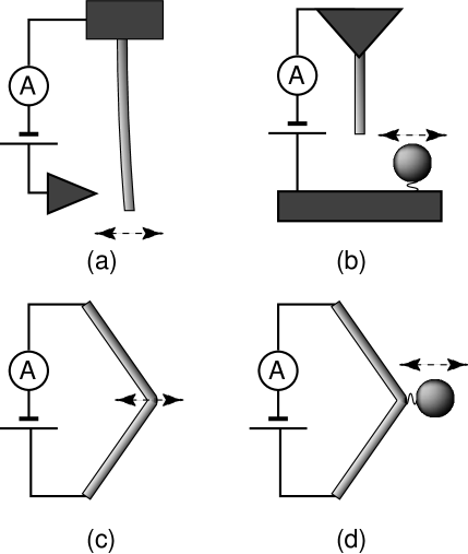
FIG. 1.: Experimental realizations of the model.

We use a Keldysh formalism[19]. Our procedure closely follows that used to study noise in Luttinger liquid tunneling[20]. Let us suppose that initially the oscillator and leads are decoupled, with density matrices $\rho_{0}$ for the oscillator and $\rho^{L}_{1,2}$ for the leads, so that the full density matrix $\rho=\rho_{0}\otimes\rho^{L}_{1}\otimes\rho^{L}_{2}$. For now, we assume that the leads are at zero temperature. After the interaction between systems is turned on at time $t=-\infty$, the systems become coupled. Define the scattering operator ${\cal S}$ by

$${\cal S}=T_{c}\,e^{-i\int\limits_{\infty}^{-\infty}{\cal H}{\rm d}t}e^{-i\int\limits_{-\infty}^{\infty}{\cal H}{\rm d}t}\equiv 1,$$ (3)

where the operator $T_{c}$ denotes time ordering along the Keldysh contours. Points along the forward branch ($-\infty\rightarrow\infty$) are ordered with increasing times, while those in the return ($\infty\rightarrow-\infty$) are ordered with decreasing times, with those in the return branch ordered after those in the forward branch. We will occasionally use a superscript $f,r$ on $t$ to indicate to which contour $t$ belongs. The expectation value of any product of operators $O(t_{1}),O(t_{2}),...$ can be obtained by

$$\langle O(t_{1})O(t_{2})...\rangle={\rm Tr}\Bigl{\{}\rho\Bigl{(}T_{c}\,O(t_{1}^{f})O(t_{2}^{f})...{\cal S}\Bigr{)}\Bigr{\}},$$ (4)

where we work in the Schroedinger representation throughout.

Tracing out the Luttinger liquids, we obtain the new scattering operator

$${\cal S}_{\rm eff}=T_{c}\,e^{-i\int\limits_{\infty}^{-\infty}{\cal H}_{0}{\rm d}t}e^{-i\int\limits_{-\infty}^{\infty}{\cal H}_{0}{\rm d}t}\times$$ (5)

$$e^{\pm\frac{1}{2}\int\limits_{-\infty}^{\infty}{\rm d}t_{1}{\rm d}t_{2}\,\Omega(t_{1})\Omega(t_{2})\frac{2\cos{(\mu(t_{1}-t_{2}))}}{(\epsilon\pm i(t_{2}-t_{1}))^{\alpha+2}}+...},$$ (6)

where the plus sign is chosen before the integral over $t_{1},t_{2}$ if $t_{1},t_{2}$ are in different branches and the minus sign is chosen if they are in the same branch. The $\pm$ sign in the denominator of the exponential is taken positive if $t_{2}$ is after $t_{1}$ and negative if $t_{2}$ is before $t_{1}$. We have used $\langle T(t_{1})T(t_{2})\rangle_{L}=2\cos{(\mu(t_{1}-t_{2}))}/(\epsilon\pm i(t_{2}-t_{1}))^{\alpha+2}$, where the expectation value $\langle\rangle_{L}$ for the leads is the expectation value for decoupled Luttinger liquids at zero temperature[20]. In this expectation value, there is an additional factor dependent on the density of states, which may be absorbed into the normalization of $\Omega$. The $...$ in Eq. (5) denote terms higher order in $\Omega$. Assuming $\Omega^{2}\mu^{\alpha}<<1$, these higher order terms may be neglected by a power counting, valid for $\alpha>0$; for $\alpha=0$, there may be logarithmic infrared divergences which upset this naive power counting, and in this case we must also assume a sufficiently large voltage to neglect these terms.

The expectation value of an operator $O(t)$ becomes

$$\langle O(t)\rangle={\rm Tr}\Bigl{\{}\rho_{0}\Bigl{(}T_{c}\,\tilde{O}(t){\cal S}_{\rm eff}\Bigr{)}\Bigr{\}}=\langle\tilde{O}(t)\rangle,$$ (7)

where we have defined $\tilde{O}=$

$$\langle O(t_{1}^{f})\rangle_{L}\mp\int{\rm d}ti\Omega(t)\langle O(t_{1}^{f})T\rangle_{L}+...\quad.$$ (8)

Here the $...$ denote connected expectation values which are higher order in $\Omega$, and where $\mp$ is chosen negative for $t$ on the forward contour and positive for $t$ on the return contour. The operator $\tilde{O}$ depends only on the oscillator coordinates and not on the leads.

The exponential in Eq. (5) involves a product $\Omega(t_{1})\Omega(t_{2})$, where $t_{1},t_{2}$ may be on either the forward or return contour. We introduce $\Omega^{s}(t_{1})=\Omega(t_{1}^{f})+\Omega(t_{1}^{r}),\Omega^{a}(t_{1})=\Omega(t_{1}^{f})-\Omega(t_{1}^{r})$. Then, $\pm\Omega(t_{1})\Omega(t_{2})\frac{2\cos{(\mu(t_{1}-t_{2}))}}{(\epsilon\pm i(t_{2}-t_{1}))^{\alpha+2}}=$

$$-\Omega^{a}(t_{1})\Omega^{a}(t_{2}){\rm Re}\Bigl{(}\frac{2\cos{(\mu(t_{1}-t_{2}))}}{(\epsilon+i|t_{2}-t_{1}|)^{\alpha+2}}\Bigr{)}$$ (9)

$$-2\Omega^{a}(t_{1})\Omega^{s}(t_{2})\theta(t_{1}-t_{2}){\rm Im}\Bigl{(}\frac{2\cos{(\mu(t_{1}-t_{2}))}}{(\epsilon+i|t_{2}-t_{1}|)^{\alpha+2}}\Bigr{)}.$$ (10)

Again assuming that $\Omega^{2}\mu^{\alpha}<<1$, we can make a further simplification in the exponential of Eq. (5), by using the Bloch-Redfield approximation[22], that $\Omega^{a,s}(t_{2})=e^{i{\cal H}_{0}(t_{2}-t_{1})}\Omega^{a,s}(t_{1})e^{-i{\cal H}_{0}(t_{2}-t_{1})}$. Corrections to the Bloch-Redfield approximation arise if operators $\Omega$ are inserted between $t_{1},t_{2}$; such corrections to ${\cal S}_{\rm eff}$ will be of order $|t_{2}-t_{1}|\Omega^{2}\mu^{\alpha+1}$. Let us write $\Omega=\Omega_{ij}$, where $i,j$ denote eigenstates of ${\cal H}_{0}$ with energies $E_{i,j}$. Then, integrating over $t_{2}$,

$${\cal S}_{\rm eff}=T_{c}\,e^{-i\int\limits_{\infty}^{-\infty}{\cal H}_{0}{\rm d}t}e^{-i\int\limits_{-\infty}^{\infty}{\cal H}_{0}{\rm d}t}\times$$ (11)

$$e^{\frac{1}{2}\int\limits_{-\infty}^{\infty}{\rm d}t\,\Bigl{(}\Omega^{a}(t)\Omega_{ij}^{s}(t)A(\mu,E_{i}-E_{j})-\Omega^{a}(t)\Omega_{ij}^{a}(t)S(\mu,E_{i}-E_{j})\Bigr{)}},$$ (12)

where we define $S(\mu,\Delta E)=\int_{-\infty}^{\infty}2\cos{(\mu t)}e^{i\Delta Et}{\rm Re}\bigl{[}(\epsilon+i|t|)^{-\alpha-2}\bigr{]}{\rm d}t$, $A(\mu,\Delta E)=-2\int_{-\infty}^{0}2\cos{(\mu t)}e^{i\Delta Et}{\rm Im}\bigl{[}(\epsilon+i|t|)^{-\alpha-2}\bigr{]}{\rm d}t$. The terms in $\Omega^{a}\Omega^{a}$ in Eq. (11) produce decoherence, and are equivalent to averaging over a randomly fluctuating field coupled to $\Omega$, while the terms $\Omega^{a}\Omega^{s}$ produce dissipation.

Taking $|E_{i}-E_{j}|<\mu$, so that the correct poles in the integrals for $A,S$ are determined by the sign of $\mu$, one finds that

$$S(\mu,\Delta E)=\frac{1}{2}\Bigl{(}I(\mu+\Delta E)+I(\mu-\Delta E)\Bigr{)}$$ (13)

$$A(\mu,\Delta E)=\frac{1}{2}\Bigl{(}I(\mu+\Delta E)-I(\mu-\Delta E)\Bigr{)}+...,$$ (14)

where $...$ denotes imaginary terms, possibly singular as $\epsilon\rightarrow 0$, which may be absorbed into a renormalization of ${\cal H}_{0}$, and hence dropped. We have defined $I(\mu)=2\pi\mu^{\alpha+1}/\Gamma(\alpha+2)$. Eqs. (11,13) are the main results.

Average Current and Noise— Here $qI(\mu)$ is equal to the current[23] flowing at $\Omega=1$. We now recompute the current within the present formalism, in order to obtain corrections to the current due to fluctuations in $\Omega$. The current operator at time $t^{f}=0$ is $J(0^{f})=qi\Omega(0^{f})(\Psi^{\dagger}_{1}(0,0^{f})\Psi_{2}(0,0^{f})-h.c.)$. From Eqs. (7,8), the leading contribution to $\langle J\rangle$ is of order $\Omega^{2}$, $\pm iq\int_{-\infty}^{\infty}{\rm d}t\,\langle\Omega(t)\Omega(0^{f})\rangle 2\sin{(\mu t)}/(\epsilon\pm it)^{\alpha+2}$. This vanishes when integrated over $t$ on the forward contour, so we can assume that $t$ is on the reverse contour. Applying the same Bloch-Redfield approximation, we get $q\int_{-\infty}^{\infty}{\rm d}te^{i(E_{i}-E_{j})t}\langle\Omega(t)\Omega(0^{f})\rangle 2\sin{(\mu t)}/(\epsilon+it)^{\alpha+2}$. Doing this integral yields

$$\langle J\rangle=q\langle\Omega_{ij}(0)\Omega(0)\rangle\frac{2\pi}{\Gamma(\alpha+2)}(\mu+E_{i}-E_{j})^{\alpha+1}.$$ (15)

We now consider fluctuations in the current, $\langle J(t_{1}^{f})J(t_{2}^{f})\rangle$. The order $\Omega^{2}$ contribution to the current-current correlation function, from Eq. (7), is given by

$$q^{2}\langle\Omega(t_{1}^{f})\Omega(t_{2}^{f})\rangle\frac{2\cos(\mu(t_{2}-t_{1}))}{(\epsilon+i|t_{2}-t_{1}|)^{2+\alpha}},$$ (16)

This represents the shot noise in the tunnel junction slightly modulated by oscillator. To next order in $\Omega^{2}$, from Eq. (7), we must compute

$$-\pm\pm\frac{q^{2}}{2}\int\limits_{-\infty}^{\infty}{\rm d}t_{3}\,{\rm d}t_{4}\,\Omega(t_{1}^{f})\Omega(t_{2}^{f})\Omega(t_{3})\Omega(t_{4})\rangle\times$$ (17)

$$\langle T(t_{1}^{f})T(t_{2}^{f})T(t_{3})T(t_{4})\rangle_{L}.$$ (18)

Even for $c$-number $\Omega$, the calculation of Eq. (17) is involved[20]; in this case, the calculation yields a result of order $\mu^{2\alpha}\Omega^{4}|t_{2}-t_{1}|^{-2}$, plus terms with lower powers of $\mu$. However, for operator $\Omega$, there is a contribution from Eq. (17) which is of order $\mu^{2\alpha+2}$, which will dominate over the previous contribution for $|t_{2}-t_{1}|>>\mu^{-1}$, the time regime we now consider.

The expectation value $\langle T(t_{1}^{f})T(t_{2}^{f})T(t_{3})T(t_{4})\rangle_{L}=\langle T(t_{1}^{f})T(t_{3})\rangle_{L}\langle T(t_{2}^{f})T(t_{4})\rangle_{L}+t_{3}\leftrightarrow t_{4}+connected$. The last term, a connected expectation value of $4$ $T$-operators, gives the contribution of order $\mu^{2\alpha}\Omega^{4}|t_{2}-t_{1}|^{-2}$ to Eq. (17). We ignore this, and consider only the other terms. Integrating over $t_{3},t_{4}$, and applying a similar procedure to that used to calculate the current above, we arrive at the following contribution to $\langle J(t_{1})J(t_{2})\rangle$:

$$q^{2}(\frac{2\pi}{\Gamma(\alpha+2)})^{2}(\mu+E_{i}-E_{j})^{\alpha+1}(\mu+E_{j}-E_{k})^{\alpha+1}$$ (19)

$$\langle\Omega_{ij}(t_{1}^{r})\Omega_{jk}(t_{2}^{r})\Omega(t_{2}^{f})\Omega(t_{1}^{f})\rangle.$$ (20)

For the expectation value $\langle T(t_{1}^{f})T(t_{3})\rangle_{L}\langle T(t_{2}^{f})T(t_{4})\rangle_{L}$ to be significant, $t_{1}-t_{3}\sim\mu^{-1}$, $t_{2}-t_{4}\sim\mu^{-1}$, justifying the application of the Bloch-Redfield approximation. For $|t_{2}-t_{1}|>>\mu^{-1}$, this approximation does not change the time ordering of $t_{3},t_{4}$. As claimed, Eq. (19) is of order $\mu^{2\alpha+2}$, reflecting a modulation of the current[7] by the oscillator. Eq. (19) decays on a time scale of order the inverse damping coefficient, $1/\gamma$, of the oscillator. In the case of $c$-number $\Omega$, this term is neglected: when computing $\langle JJ\rangle-\langle J\rangle\langle J\rangle$, it cancels.

Density Matrix— For $\Delta E<<\mu$, it is possible to write the results above in a compact form. Define $\rho(t)$ to be the density matrix for the oscillator at given time $t$. Then use Eqs. (7,11) to compute $\langle\dot{\tilde{O}}(t^{f})\rangle$ for any operator $\tilde{O}$; the result is be a linear differential equation for the expectation values. Then use $\langle\dot{\tilde{O}}(t^{f})\rangle\equiv{\rm Tr}(\dot{\rho}(t)\tilde{O})$ to derive the equation for the density matrix:

$$\dot{\rho}=-i\Bigl{[}{\cal H}_{0},\rho\Bigr{]}+\frac{1}{2}\frac{{\rm d}I}{{\rm d}\mu}\Bigl{[}\Omega,\Bigl{\{}\Lambda,\rho\Bigr{\}}\Bigr{]}-\frac{I}{2}\Bigl{[}\Omega,\Bigl{[}\Omega,\rho\Bigr{]}\Bigr{]},$$ (21)

with $\Lambda=[{\cal H}_{0},\Omega]$. Comparing to the results for Fermi liquid leads[9], the effective temperature of the oscillator, determined by the ratio of the third (decoherence) term to the second (dissipation) term in Eq. (21), is

$$T_{\rm eff}=(\alpha+1)^{-1}qV/2.$$ (22)

For the current, we find $\langle J\rangle=q\langle\Omega^{2}\rangle I(\mu)+q\langle\Lambda\Omega\rangle{\rm d}I/{\rm d}\mu$.

Spectral Representation— While these results were derived for Luttinger liquid leads, they are more general. Assuming sufficiently small $\Omega$, we find Eq. (5) with $2\cos{(\mu(t_{1}-t_{2}))}/(\epsilon\pm i(t_{2}-t_{1}))^{\alpha+2}$ replaced by the appropriate expectation value in the leads, $\langle T(t_{1})T(t_{2})\rangle_{L}$. Let the density of states (particle and hole, respectively) at energy $E$ be $\rho^{p,h}_{1,2}(E)$ in leads $1,2$ respectively. Then, defining $\rho^{p}(E)=\int{\rm d}E_{1}\,\rho^{p}_{1}(E_{1})\rho^{h}_{2}(E-E_{1}),$ $\rho^{h}(E)=\int{\rm d}E_{1}\,\rho^{h}_{1}(E_{1})\rho^{p}_{2}(E-E_{1})$, the expectation value is $\int{\rm d}E\,(\rho^{p}(E)e^{\mp i(E+\mu)(t_{1}-t_{2})}+\rho^{h}(E)e^{\mp i(E-\mu)(t_{1}-t_{2})}),$ with the minus sign chosen if $t_{1}$ is after $t_{2}$ and the plus sign otherwise. Then going through the same steps, we find Eq. (11,13) in general, with $I(\mu)$ replaced by the appropriate current-voltage characteristic of the device: $I(\mu)=2\pi(\rho^{p}(-\mu)+\rho^{h}(\mu))$. The relation between $S,A$ and $I$ generalizes the fluctuation-dissipation relation derived between noise and current[24]. For $\Delta<<\mu$, we arrive at Eq. (1).

Applications— We now consider the specific case of a harmonic oscillator with frequency $\omega_{0}$ and mass $m$, linearly coupled to the tunneling, $\Omega=\Omega_{0}+cx$. We consider a regime for which the $\Omega_{0}$ term dominates and the oscillator coordinate $x$ only weakly modulates the current. For $\mu>\omega_{0}$, the average current is

$$J(\mu)=q[I\Omega_{0}^{2}+\frac{c^{2}S^{2}}{2m\omega_{0}A}-\frac{c^{2}A}{2m\omega_{0}}],$$ (23)

where $I=I(\mu);S=S(\mu,\omega_{0});A=A(\mu,\omega_{0})$.

The noise spectrum can be evaluated from Eqs. (16,19). Fourier transforming Eq. (16) gives the shot noise contribution

$$q^{2}\int dte^{i\omega t}\langle\Omega(0)\Omega(t)\rangle_{L}\langle T(0)T(t)\rangle_{L}=2q^{2}\Omega_{0}^{2}I,$$ (24)

for $|\omega|\ll|\mu|$. The modulation, Eq. (17), to leading order in $c^{2}$ from Eq. (11), yields

$$\frac{q^{2}\Omega_{0}^{2}c^{4}}{m^{2}}\frac{(I+S)^{2}S-A^{2}(S+2I)}{(\omega^{2}-\omega_{0}^{2})^{2}+\gamma^{2}\omega^{2}},$$ (25)

where $\gamma=c^{2}A(\mu,\omega_{0})/(m\omega_{0})$. At the peak, the signal-to-noise ratio, Eq. (25) divided by Eq. (24), is approximately $2I^{2}/A^{2}$.

Acknowledgements— This work was supported by DOE W-7405-ENG-36, NSF DMR-0121146 (DM), and DARPA MOSAIC (IM). We thank M. Paalanen for encouragement, and K. Schwab and A. Shnirman for useful discussions.

REFERENCES

• [1] Y. Nakamura, Y.A. Pashkin, and J.S. Tsai, Nature (London) 398, 786 (1999).
• [2] D. Vion, et al., Science 296, 886 (2002).
• [3] Y. Yu, et al., Science, 296, 889 (2002).
• [4] V.B. Braginsky and F.Ya. Khalili, Quantum Measurement, (Universiy Press, Cambridge 1992).
• [5] S. A. Gurvitz, Phys. Rev. B 56, 15215 (1997); S. A. Gurvitz and Ya. S. Prager Phys. Rev. B 53, 15932 (1996).
• [6] Y. Makhlin, G. Schon, and A. Shnirman, Rev. Mod. Phys. 73, 357 (2001).
• [7] A. N. Korotkov, Phys. Rev. B 60, 5737 (1999); A. N. Korotkov and D. V. Averin, Phys. Rev. B 64, 165310 (2001).
• [8] G. Johansson, A. Käck, and G. Wendin, Phys. Rev. Lett. 88, 046802 (2002).
• [9] D. Mozyrsky and I. Martin, Phys. Rev. Lett. 89, 018301 (2002).
• [10] D. Mattis and E. Leib, J. Math. Phys 15, 609 (1965).
• [11] Z. Yao, H.W.Ch. Postma, L. Balents, and C. Dekker, Nature (London) 402, 273 (1999).
• [12] W. Apel and T. M. Rice, Phys. Rev. B 26, 7063 (1982).
• [13] D. L. Maslov and M. Stone, Phys. Rev. B 52, 5539 (1995).
• [14] M.M.J. Treacy, T.W. Ebbesen, and J.M. Gibson, Nature (London) 381, 678 (1996); R.S. Ruoff and D.C. Lorents, Carbon 33, 925 (1995).
• [15] J.H. Hafner, C.L. Cheung, and C.M. Leiber, Nature (London) 398, 761 (1999).
• [16] C. L. Kane and M. P. A. Fisher, Phys. Rev. Lett. 68, 1220 (1992).
• [17] D. Sánchez-Portal, et al., Phys. Rev. B 59, 12678 (1999).
• [18] S.S. Wong, et al., Nature (London) 394, 52 (1998).
• [19] L. V. Keldysh, Soviet Phys. JETP 20, 1018 (1965).
• [20] C. D. Chamon, D. E. Freed, and X. G. Wen, Phys. Rev. B 51, 2363 (1995).
• [21] C. Kane, L. Balents, and M. P. A. Fisher, Phys. Rev. Lett. 79, 5086 (1997).
• [22] F. Bloch, Phys. Rev. 70, 460 (1946); A.G. Redfield, IBM J. Res. Dev. 1, 19 (1957).
• [23] X. G. Wen, Phys. Rev. B 44, 5708 (1991).
• [24] D. Rogovin and D.J. Scalapino, Ann. Phys. (N.Y.) 86, 1 (1974).