A New Method to Estimate the Noise in Financial Correlation Matrices

Abstract

Financial correlation matrices measure the unsystematic correlations between stocks. Such information is important for risk management. The correlation matrices are known to be “noise dressed”. We develop a new and alternative method to estimate this noise. To this end, we simulate certain time series and random matrices which can model financial correlations. With our approach, different correlation structures buried under this noise can be detected. Moreover, we introduce a measure for the relation between noise and correlations. Our method is based on a power mapping which efficiently suppresses the noise. Neither further data processing nor additional input is needed.

1 Introduction

There are different kinds of risk in a stock portfolio, for example, a systematic one due to the general trends in the economy affecting the entire market, and an unsystematic one due to events affecting only segments of the whole market under consideration, such as the companies within the same industrial branch or in one country [1]. All this is borne out in the time series of the stocks. In a more general framework, the term “stock of a company” should be replaced by “risk factor”. The corresponding portfolios of a bank or an investment company can contain hundreds or thousands of financial instruments, depending on many different risk factors [1]. However, to be explicit, we will use the term “stocks” instead of “risk factors”. Banks or portfolio managers are particularly interested in the unsystematic correlations [2, 3]. We refer to them simply as correlations from now on. The elements of the correlation matrix are given through the time average over a product of the properly normalized time series for two stocks. The number of companies considered defines the size of this correlation matrix. We will assume that this number is large enough for a statistical analysis.

In recent years, it was shown that the true correlations one is interested in can be buried under noise in the commonly used correlation matrices: Laloux et al. [4] studied an empirical correlation matrix and found that the bulk part of its spectral density can be modeled by a purely random matrix. Plerou et al. [5] worked out spectral fluctuations and also found that they are compatible with random matrix statistics. Random matrices are often used statistical models for quantum chaotic or related spectral problems, for reviews see Refs. [6, 7, 8]. The presence of random matrix features was coined noise dressing of financial correlations. Burda et al. [9] designed a proper model involving random Levy matrices. In practice, such noise can appear if the length of the time series employed to construct the correlation matrices is too short. Gopikrishnan et al. [10] developed a method to reduce the noise by taking advantage of the fact that large eigenvalues outside the bulk of the spectral density can be associated with industrial branches. These authors [10] used this for portfolio optimization, see also Ref. [11]. The identification of branches through stock correlations was also studied by Mantegna [12].

Here, we present a new approach to identify and estimate the noise and, thereby, also the strength of the true correlations. As we do not use the large eigenvalues outside the bulk of the spectral density, our method is an alternative and a complement to the approach of Ref. [10]. It will be particularly useful if some of the large eigenvalues are not large enough to lie outside the bulk of the spectral density. Our method is based on a power mapping. It does not require any further data processing or any other type of input. To the best of our knowledge, it seems to be a new technique for the analysis of correlation matrices in time series problems. We have three goals: first, we develop an alternative method for noise identification, second, we introduce the power mapping as a new mathematical–statistical technique and discuss its features in some detail, third, we present our findings in a self–contained way to make possible a transfer to other time series problems and the corresponding correlation matrices.

The article is organized as follows. In Sec. 2, we outline the stochastic model, including a review of correlation matrices and a discussion of the noise dressing phenomenon. We study the dependence of the spectral density as a function of the length of the time series in Sec. 3. In Sec. 4, we introduce the power mapping and use it to identify and estimate the noise. We summarize and conclude in Sec. 5. Three more detailed discussions are given in the appendix.

2 Stochastic Model

We formulate the model for financial correlations in Sec. 2.1. Since we also aim at a heuristic analytical treatment later on, we do that in some detail. Correlation matrices and noise dressing are discussed in Secs. 2.2 and 2.3, respectively.

2.1 Normalized Time Series for Correlated Stocks

Most models for time series $S(t)$ of stocks [13, 14, 15, 16] have a random component, involving a random number $\varepsilon$ and a volatility constant $\sigma^{2}$, and a non–random component, the drift part, involving a drift constant $\mu$. Geometric Brownian motion

$$\frac{dS}{S}=\mu dt+\sigma\varepsilon\sqrt{dt}$$ (1)

is particularly popular. The dimensionless quantity $dS/S$ is referred to as return. Due to the central limit theorem, geometric Brownian motion leads, largely independently of the distribution for the random numbers $\varepsilon$, to a log–normal distribution of the stock prices. This is in fair agreement with the empirical distributions for price changes about one day and greater [17, 18]. The tails of the empirical distributions are, in general, much fatter [13, 14]. To describe this, one uses, for example, autoregressive processes which take into account that the volatility is also a fluctuating quantity, see the discussion in Ref. [13]. In the present context of correlations, however, it suffices to model the time series in the spirit of geometric Brownian motion. In economics, one wishes to measure the correlations independent of the drift. Thus, one usually takes the logarithms or the logarithmic differences of the time series to remove the exponential trend in the data due to the drift. Moreover, one normalizes the data to zero mean value and unit variance.

In view of these requirements, Noh [19] suggested a proper model to study financial correlations. From an economics viewpoint, it is of the one–factor type and can be interpreted as an application of the arbitrage pricing model due to Ross [20], see also the discussion in A. From a physics viewpoint, as pointed out in Refs. [21, 22], Noh’s model has much in common with certain models involving interacting Potts spins [23]. Consider a market involving $K$ companies, labeled $k=1,\ldots,K$, and $B$ industrial branches, labeled $b=1,\ldots,B$. The companies within the same industrial branch are assumed to be correlated. The companies are ordered in such a way that the indices $k$ of companies within the same branch follow each other. For example, we have $K=50$ companies and $B=3$ branches and we assume that the first branch with $b=1$ consists of the first $\kappa_{1}=5$ companies, the second branch with $b=2$ consists of the next $\kappa_{2}=12$ companies, the third branch with $b=3$ consists of the next $\kappa_{3}=8$ companies, and, finally, we assume that the remaining $\kappa=25$ companies are in no branch. The branch index $b$ is viewed as a function of the company index $k$, i.e. we have $b=b(k)$. For the $\kappa$ companies which are not in any branch, we set $b=b(k)=0$. We refer to $\kappa_{b}$ as to the size of the industrial branch $b$. Obviously, we have

$$\sum_{b=1}^{B}\kappa_{b}+\kappa=K\ .$$ (2)

Of course, we assume that $\kappa_{b}>1,\ b=1,\ldots,B$. The number $\kappa$ can be any non–negative integer, including zero.

The normalized time series $M_{k}(t),\ k=1,\ldots,K$ of the returns for the $K$ companies are modeled as the sum of two purely random contributions: the first one models the correlations within a given branch and is thus common to this branch, involving random numbers $\eta_{b}(t)$, the second one is specific for the company and involves random numbers $\varepsilon_{k}(t)$,

$$M_{k}(t)=\sqrt{\frac{p_{b(k)}}{1+p_{b(k)}}}\eta_{b(k)}(t)+\frac{1}{\sqrt{1+p_{b(k)}}}\varepsilon_{k}(t)\ .$$ (3)

The two contributions are weighted with a parameter $p_{b(k)}$, common to all companies in the branch $b$. We assume that the $\eta_{b(k)}(t)$ and the $\varepsilon_{k}(t)$ are uncorrelated and standard normal distributed with zero mean value. The weights are assumed to be positive with $p_{b(k)}\geq 0$. Since the distributions are symmetric, this is the most general form of the weights. In the case that $k$ is not in any branch, i.e. for $b=0$, we set $p_{b(k)}=0$. Here, we use discrete time steps and normalize the time units such that $dt=1$. The time series $M_{k}(t)$ consist of $T$ time values at $t=1,\ldots,T$.

2.2 Correlation Matrices

The time average of a function $F(t)$ over the time series is defined as

$$\langle F(t)\rangle_{T}=\frac{1}{T}\sum_{t=1}^{T}F(t)\ ,$$ (4)

which depends on the length $T$ of the time series. If the time series are infinitely long, $T\to\infty$, we have

$$\langle M_{k}(t)\rangle_{\infty}=0\qquad{\rm and}\qquad\langle M_{k}^{2}(t)\rangle_{\infty}=1\ .$$ (5)

Here, we simply used $\langle\eta_{b(k)}(t)\rangle_{\infty}=0$, $\langle\varepsilon_{k}(t)\rangle_{\infty}=0$ and $\langle\eta_{b(k)}(t)\eta_{b(l)}(t)\rangle_{\infty}=\delta_{b(k)b(l)}$, $\langle\eta_{b(k)}(t)\varepsilon_{l}(t)\rangle_{\infty}=0$, $\langle\varepsilon_{k}(t)\varepsilon_{l}(t)\rangle_{\infty}=\delta_{kl}$.

The correlation coefficient between two companies labeled $k$ and $l$ is the average over the product of the two normalized time series,

$$C_{kl}(T)=\frac{1}{T}\sum_{t=1}^{T}M_{k}(t)M_{l}(t)=\langle M_{k}(t)M_{l}(t)\rangle_{T}\ .$$ (6)

If one views the numbers $M_{k}(t)$ as the entries of a $K\times T$ rectangular matrix $M$, one has

$$C(T)=\frac{1}{T}MM^{\dagger}=\langle M(t)M^{\dagger}(t)\rangle_{T}$$ (7)

for the $K\times K$ correlation matrix $C$. As these averages depend on the length $T$ of the time series, we add the argument $T$ to the correlation matrix. Within our model outlined above, one finds for infinitely long time series [21], $T\to\infty$,

$$C_{kl}(\infty)=\lim_{T\to\infty}C_{kl}(T)=\frac{1}{1+p_{b(k)}}\left(p_{b(k)}\delta_{b(k)b(l)}+\delta_{kl}\right)\ .$$ (8)

Thus, the matrix $C(\infty)$ consists of $B$ square blocks on the diagonal of dimensions $\kappa_{b}\times\kappa_{b}$ with off–diagonal entries $p_{b}/(1+p_{b})$ for branch $b$, and a $\kappa\times\kappa$ unit matrix for the companies which are in no branch. The diagonal entries are all unity. All other entries are zero: the correlation coefficients between companies which are not in any branch, those between companies belonging to different branches and those between a company which is in a branch and another one which is not. Some issues related to the normalization of correlation matrices are discussed in A.

2.3 Noise Dressing in the Model

If the time series have only a finite length, $T<\infty$, it is obvious that the averages $\langle\eta_{b(k)}(t)\eta_{b(l)}(t)\rangle_{T}$, $\langle\eta_{b(k)}(t)\varepsilon_{l}(t)\rangle_{T}$ and $\langle\varepsilon_{k}(t)\varepsilon_{l}(t)\rangle_{T}$ give neither zero nor unity, but some finite numbers. This describes the noise dressing of financial correlation matrices which was found in Ref. [4] in the framework of Noh’s model. Due to the finiteness of the time series, there is a purely random offset to every correlation coefficient, burying the true correlation coefficient which would be found if the time series were sufficiently long.

As we aim at a analytical discussion later on, we formulate the noise dressing more quantitatively. We employ a standard result of mathematical statistics [24]: Consider two time series of uncorrelated random numbers $\alpha_{k}(t)$ and $\alpha_{l}(t),\ t=1,\ldots,T$ with standard normal distributions and zero mean value. The average $\langle\alpha_{k}(t)\alpha_{l}(t)\rangle_{T}$ is a random number, following a Gauss distribution centered at mean value unity with variance $2/T$, if $k=l$, and following a Gauss distribution centered at mean value zero with variance $1/T$, if $k\neq l$. Hence, we can write this average to leading order in $T$ as

$$\langle\alpha_{k}(t)\alpha_{l}(t)\rangle_{T}=\delta_{kl}+\sqrt{\frac{1+\delta_{kl}}{T}}a_{kl}\ ,$$ (9)

where the $a_{kl}$ are uncorrelated random numbers, independent of $T$, with standard normal distribution and zero mean value. This yields for the correlation coefficients the expression

$$C_{kl}(T) = \sqrt{\frac{p_{b(k)}}{1+p_{b(k)}}}\sqrt{\frac{p_{b(l)}}{1+p_{b(l)}}}\Biggl{(}\delta_{b(k)b(l)}+\sqrt{\frac{1+\delta_{b(k)b(l)}}{T}}a_{b(k)b(l)}\Biggr{)}$$ (10)

$$\quad+\frac{1}{\sqrt{1+p_{b(k)}}}\frac{1}{\sqrt{1+p_{b(l)}}}\Biggl{(}\delta_{kl}+\sqrt{\frac{1+\delta_{kl}}{T}}a_{kl}\Biggr{)}$$

$$\quad+\sqrt{\frac{p_{b(k)}}{1+p_{b(k)}}}\frac{1}{\sqrt{1+p_{b(l)}}}\frac{1}{\sqrt{T}}a_{b(k)l}$$

$$\quad+\sqrt{\frac{p_{b(l)}}{1+p_{b(l)}}}\frac{1}{\sqrt{1+p_{b(k)}}}\frac{1}{\sqrt{T}}a_{kb(l)}$$

to leading order in $T$. The first two terms stem from the averages $\langle\eta_{b(k)}(t)\eta_{b(l)}(t)\rangle_{T}$ and $\langle\varepsilon_{k}(t)\varepsilon_{l}(t)\rangle_{T}$, the last two from the interference averages $\langle\eta_{b(k)}(t)\varepsilon_{l}(t)\rangle_{T}$. There are four sets of random numbers, $a_{b(k)b(l)}$, $a_{b(k)l}$, $a_{kb(l)}$ and $a_{kl}$, respectively. These sets are understood to be different from each other. To avoid a cumbersome notation, we do not add further indices to specify that. For example, the number $a_{b(1)b(1)}$ is different from $a_{11}$. As required, the limit $T\to\infty$ of Eq. (10) correctly yields Eq. (8).

3 Spectral Density and Length of the Time Series

As shown in Ref. [4], the spectral density is a well suited observable to study the noise dressing of empirical correlation matrices. In Sec. 3.1, we numerically investigate the spectral density of our model as a function of the length $T$ of the time series. We support our findings by an analytical discussion in Sec. 3.2.

3.1 Numerical Simulation

As the number of companies in the analysis [4, 5] of real market data is several hundreds, we choose this number as $K=508$ for our simulation. We assume that there are $B=6$ industrial branches whose sizes $\kappa_{b}$ and weights $p_{b}$ are listed in table 1. Since Noh [19] showed that the choice

$$p_{b}=1-\frac{1}{\kappa_{b}}$$ (11)

leads to spectral densities which are in agreement with the empirical data [4, 5], we use the same parameterization here. In addition, we have $\kappa=256$ companies which are not in any branch.

We simulate the correlation matrices $C(T)$ for four different lengths $T=1650,5000,20000,50000$ of the time series, calculate the eigenvalues $\lambda_{k},\ k=1,\ldots,K$ and work out the spectral densities $\rho_{T}(\lambda)$. The results are shown in figure 1. As already observed by Noh [19], the first density $\rho_{1650}(\lambda)$ for the shortest time series with $T=1650$ resembles very much the densities of the empirical correlation matrices found in Refs. [4, 5]. There is a bulk

Table 1: The sizes $\kappa_{b}$ and the weights $p_{b}=1-1/\kappa_{b}$ for the $B=6$ industrial branches used in the numerical simulation.

• $b$	1	2	3	4	5	6
  $\kappa_{b}$	4	8	16	32	64	128
  $p_{b}$	0.75	0.88	0.94	0.97	0.98	0.99

spectrum in the interval $0<\lambda<2$. Moreover, a number of isolated peaks in the interval $2<\lambda<70$ is seen. Each of these large eigenvalues corresponds to an individual industrial branch. For increasing lengths $T$, the isolated peaks are stable, but the bulk spectrum separates into two groups of eigenvalues. The left group is roughly centered around $\lambda=1/2$, the right one around $\lambda=1$. We will see in the analytical discussion to be performed in Sec. 3.2 that the left group can clearly be associated with the true correlations due to the industrial branches, while the right group only represents noise around the trivial self–correlation of the companies for $k=l$.

3.2 Analytical Discussion

For infinitely long time series, $T\to\infty$, the correlation matrix $C(\infty)$ is block diagonal according to Eq. (8), and the spectrum of the eigenvalues $\lambda_{k}(\infty),\ k=1,\ldots,K$ is easily calculated. For every branch $b$, we have $\kappa_{b}-1$ degenerate eigenvalues $1/(1+p_{b})$ and one numerically much larger eigenvalue $(1+\kappa_{b}p_{b})/(1+p_{b})$ which is for large size $\kappa_{b}$ roughly proportional to $\kappa_{b}$. Moreover, there are $\kappa$ degenerate eigenvalues which are unity for the companies which are in no branch. Thus, the spectral density is given by

$$\rho_{\infty}(\lambda) = \sum_{b=1}^{B}(\kappa_{b}-1)\delta\left(\lambda-\frac{1}{1+p_{b}}\right)$$ (12)

$$+\sum_{b=1}^{B}\delta\left(\lambda-\frac{1+\kappa_{b}p_{b}}{1+p_{b}}\right)+\kappa\delta\left(\lambda-1\right)\ .$$

This formula helps to understand the last density for the longest time series with $T=50000$ in figure 1. The first term corresponds to the left group, representing the true correlations. The second term of the $B$ large eigenvalues yield the isolated peaks of the spectra. The last term in the formula represents the noise peaked at unity. The eigenvectors $u_{k}(\infty),\ k=1,\ldots,K$ can also be calculated in a straightforward manner for $T\to\infty$.

The density (12) is smeared out for finite time series, $T<\infty$. To estimate the resulting noisy density $\rho_{T}(\lambda)$ to leading order in $T$, we write the correlation matrix in the form

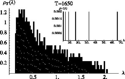
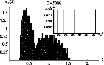
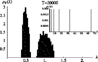
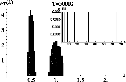
Figure 1: Spectral densities $\rho_{T}(\lambda)$ of simulated correlation matrices. The length $T$ of the time series increases from top to bottom according to $T=1650,5000,20000,50000$. The presentation of every density is split into the regions $0\leq\lambda\leq 2.2$ and $2.2\leq\lambda\leq 70$. The densities are given in units of $K$.

$C(T)=C(\infty)+C_{1}/\sqrt{T}$ where $C_{1}$ can be read off from the expansion (10). We also write $\lambda_{k}(T)=\lambda_{k}(\infty)+\lambda_{1,k}/\sqrt{T}$ for the eigenvalues and $u_{k}(T)=u_{k}(\infty)+u_{1,k}/\sqrt{T}$ for the eigenvectors. One quickly finds $\lambda_{1,k}=u_{k}^{\dagger}(\infty)C_{1}u_{k}(\infty)$. Since the elements of every $u_{k}(\infty)$ are numbers depending on the weights $p_{b}$ and the sizes $\kappa_{b}$, every coefficient $\lambda_{1,k}$ is, according to Eq. (10), a linear combination of the standard normal distributed random numbers $a_{b(k)b(l)}$, $a_{b(k)l}$, $a_{kb(l)}$ and $a_{kl}$. Hence, it is itself a Gaussian distributed random number $a_{k}$ with zero mean value and a variance $v_{k}^{2}$ which is some function of the $p_{b}$ and the $\kappa_{b}$. We arrive at

$$\lambda_{k}(T)=\lambda_{k}(\infty)+\frac{v_{k}}{\sqrt{T}}a_{k}$$ (13)

for $k=1,\ldots,K$ to leading order in $T$. We notice that, in this expansion to order $1/\sqrt{T}$, the Gaussian random variables $a_{k}$ are uncorrelated. The effect of the smearing out, i.e. of the noise in the model, is marginal for the $B$ numerically large eigenvalues $(1+\kappa_{b}p_{b})/(1+p_{b}),\ b=1,\ldots,B$. Their positions change the less, the larger the size $\kappa_{b}$. The effect of the noise is much stronger on the numerically smaller eigenvalues. Moreover, their degeneracies are lifted and distributions develop around their mean values. For the eigenvalues $1/(1+p_{b}),\ b=1,\ldots,B$ which belong to the $B$ industrial branches and, hence, describe true correlations, the mean value is

$$\mu_{B}=\frac{1}{B}\sum_{b=1}^{B}\frac{1}{1+p_{b}}\ ,$$ (14)

while it simply reads $\mu_{0}=1$ for the eigenvalues which are unity and which were generated by the time series not belonging to any branch. As the weights satisfy $p_{b}>0$ if $b=1,\ldots,B$, we always have

$$\mu_{B}<1=\mu_{0}\ .$$ (15)

This important relation implies that the centers of the distributions generated by the noise from the two set of degenerate eigenvalues are always different from each other. The distribution due to the true correlations will always be left of that which is due to trivial self–correlation for $k=l$. In the numerical simulation, we chose $p_{b}=1-1/\kappa_{b}$. Assuming that the sizes $\kappa_{b}$ are large, we find to leading order

$$\mu_{B}=\frac{1}{B}\sum_{b=1}^{B}\frac{1}{2-1/\kappa_{b}}=\frac{1}{2}+\frac{1}{4B}\sum_{b=1}^{B}\frac{1}{\kappa_{b}}\ ,$$ (16)

which explains why the distribution due to the true correlations is roughly centered around $1/2$ in figure 1.

To find an estimate for the noisy density $\rho_{T}(\lambda)$, we argue phenomenologically. Some further analytical properties are compiled in B. We first replace the first term of Eq. (12) with a Gaussian distribution centered at $\mu_{B}$,

$$G(\lambda-\mu_{B},v_{B}^{2}/T)=\sqrt{\frac{T}{2\pi v_{B}^{2}}}\exp\left(-\frac{(\lambda-\mu_{B})^{2}}{2v_{B}^{2}/T}\right)\ .$$ (17)

For its variance, we write $v_{B}^{2}/T$ where $v_{B}$ is a proper geometric average of those numbers $v_{k}$ in Eq. (13) which stem from the industrial branches. As a weight factor, we sum over the multiplicities in the degenerate case (12),

$$\sum_{b=1}^{B}(\kappa_{b}-1)=K-\kappa-B\ .$$ (18)

Similarly, we could replace the third term of Eq. (12) with a Gaussian centered at $\mu_{0}=1$. However, it is better to employ the fact the $\kappa\times\kappa$ block of the companies which are in no branch belongs to a chiral random matrix ensemble [25, 11] whose density is known [26, 27] to have the algebraic form

$$\rho_{\rm ch}(\lambda,\kappa/T)=\frac{T}{2\pi\kappa}{\rm Re\,}\frac{\sqrt{(\lambda_{+}-\lambda)(\lambda-\lambda_{-})}}{\lambda}\ .$$ (19)

where $\lambda_{\pm}$ are the largest and the smallest eigenvalues, respectively, given by

$$\lambda_{\pm}=1+\frac{\kappa}{T}\pm 2\sqrt{\frac{\kappa}{T}}\ .$$ (20)

Both of them converge to $\mu_{0}=1$ for $T\to\infty$. Outside the interval $\lambda_{-}<\lambda<\lambda_{+}$, the square root in Eq. (19) is strictly imaginary. Thus, the real part ensures that the function $\rho_{\rm ch}(\lambda,\kappa/T)$ is zero outside the supporting interval $\lambda_{-}<\lambda<\lambda_{+}$. As a weight factor, we take the multiplicity $\kappa$ in the degenerate case (12). We notice that, analogous to $v_{B}$, there would be in principle a scale $v_{0}$ entering the density $\rho_{\rm ch}(\lambda,\kappa/T)$. It would result from a proper average of those numbers $v_{k}$ in Eq. (13) which do not stem from the industrial branches. However, since we start out from normalized time series and since the weights $p_{b}$ do not contribute here, we expect $v_{0}=1$. The second term of Eq. (12) we leave unchanged, because we can ignore the shift in the positions of these largest eigenvalues. Thus, collecting everything, we find

$$\rho_{T}(\lambda) = (K-\kappa-B)G(\lambda-\mu_{B},v_{B}^{2}/T)$$ (21)

$$+\sum_{b=1}^{B}\delta\left(\lambda-\frac{1+\kappa_{b}p_{b}}{1+p_{b}}\right)+\kappa\rho_{\rm ch}(\lambda,\kappa/T)\ .$$

As the functions $G(\lambda-\mu_{B},v_{B}^{2}/T)$ and $\rho_{\rm ch}(\lambda,\kappa/T)$ are normalized to unity, the noisy density $\rho_{T}(\lambda)$ is correctly normalized to the total number $K$ of eigenvalues. We expect the formula (21) to work particularly well for large $T$. In figure 2 we fit it to the bulk part of the spectral density $\rho_{20000}(\lambda)$ for $T=20000$ which was presented in figure 1. The agreement is very good, the fit yields $v_{B}=9$.

• 

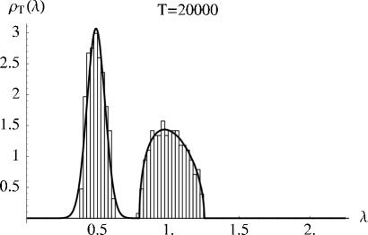
Figure 2: Bulk part of the spectral density $\rho_{20000}(\lambda)$ for $T=20000$. The phenomenological formula (21) is fitted to it. The density is given in units of $K$.

4 Noise Identification by Power Mapping

In Sec. 4.1, we introduce the power mapping and discuss its properties numerically. We give a qualitative analytical explanation in Sec. 4.2. In Sec. 4.3, we demonstrate how the power mapping can detect different correlation structures. Finally, we define a measure for the noise in Sec. 4.4.

4.1 Power Mapping

The true correlations buried under the noise become visible in the spectral density if the time series are long enough. Thus, if we found a procedure that is equivalent, in some sense, to a prolongation of the time series, we would be able to identify and quantify the noise in a given correlation matrix. In the sequel, we develop such a procedure, the power mapping. We map the correlation matrix $C(T)$ to the matrix $C^{(q)}(T)$. Here, $q$ is a positive number and the elements of $C^{(q)}(T)$ are calculated according to the definition

$$C_{kl}^{(q)}(T)={\rm sign\,}(C_{kl}(T))|C_{kl}(T)|^{q}\ .$$ (22)

Thus, the mapping preserves the sign of the matrix element $C_{kl}(T)$ and raises the modulus of it to the $q$–th power. We notice that $C^{(q)}(T)$ is the matrix of the powers of the elements of $C(T)$, but not the power of the matrix $C(T)$. This is crucial, because the spectra of $C(T)$ and $(C(T))^{q}$ are, for $q\neq 0$, related in a simple way: if $\lambda_{k},\ k=1,\ldots,K$ are the eigenvalues of $C(T)$, $\lambda_{k}^{q},\ k=1,\ldots,K$ are the eigenvalues of $(C(T))^{q}$. The spectrum of $C^{(q)}(T)$ is much more complicated and depends on the eigenvalues and the eigenvectors of $C(T)$. However, depending on the numerical value chosen for $q$, it allows one to suppress, in $C^{(q)}(T)$, certain elements of $C(T)$. This will now be demonstrated through a numerical study of the spectral densities.

We simulate correlation matrices for $K=508$ companies from time series of length $T_{0}=1650$ with the sizes $\kappa_{b}$ and the weights $p_{b}$ given in table 1. We do so to make possible a comparison with figure 1, where the impact of increasing length for the time series was studied, starting from a correlation matrix with the same sizes and weights and for the same length $T=1650$. To improve the statistical significance and to better illustrate the effect of the power mapping, we simulate an ensemble of 25 such correlation matrices from time series of length $T_{0}=1650$. We choose powers $q=1.0,1.25,1.5,1.75,2.0,2.25,2.5$ and calculate, for a fixed $q$, the 25 power mapped matrices $C^{(q)}(T)$ from the 25 matrices $C(T)$ of the ensemble. Then, the individual spectra are evaluated and the density $\rho_{T_{0}}^{(q)}(\lambda)$ results as the ensemble average. All densities are shown in figure 3.

The power mapping transforms the original density $\rho_{T_{0}}^{(1)}(\lambda)=\rho_{T_{0}}(\lambda)$ for $q=1$ into densities $\rho_{T_{0}}^{(q)}(\lambda)$ which show for intermediate values of $q$ two clearly separated peaks. The best separation is obtained near $q=1.5$. For values beyond $q=2$, the two peaks glue together again, and the separation is lost. What do these two peaks in the densities $\rho_{T_{0}}^{(q)}(\lambda)$ for $1.25\leq q\leq 2.0$ represent? — Comparison with figure 1 shows that, indeed, the left peak in figure 3 corresponds to the one for the true correlations in figure 1, while the right peak in figure 3 corresponds to the one for the noise around the trivial self–correlation of the companies for $k=l$ in figure 1. Hence, we have found the desired procedure which roughly amounts to a prolongation of the time series.

4.2 Qualitative Analytical Discussion

To leading order in the length $T$ of the time series, the $C_{kl}(T)$ are given by Eq. (10). To understand the effect of the power mapping, we distinguish three different cases in considering $|C_{kl}(T)|^{q}$. First, we power map the diagonal elements $C_{kk}(T)$. As Eq. (10) shows, the vast majority of them matrix elements will be positive if $T$ is sufficiently large. Thus, to simplify the discussion, we ignore the absolute value sign. To leading order in $T$, we have

$$(C_{kk}(T))^{q} = 1+\frac{q}{1+p_{b(k)}}\Biggl{(}\sqrt{2}p_{b(k)}a_{b(k)b(k)}+\sqrt{2}a_{kk}$$ (23)

$$\qquad+\sqrt{p_{b(k)}}(a_{b(k)k}+a_{kb(k)})\Biggr{)}\frac{1}{\sqrt{T}}\ .$$

Second, we power map the off–diagonal elements $C_{kl}(T)$ in the blocks of the industrial branches where $k\neq l$ but $b(k)=b(l)$. For the same reason as in the previous case, we ignore the absolute value sign, and find

$$(C_{kl}(T))^{q} = \left(\frac{p_{b(k)}}{1+p_{b(k)}}\right)^{q}+\frac{q(p_{b(k)})^{q-1}}{(1+p_{b(k)})^{q}}\Biggl{(}\sqrt{2}p_{b(k)}a_{b(k)b(k)}+\sqrt{2}a_{kl}$$ (24)

$$\qquad+\sqrt{p_{b(k)}}(a_{b(k)l}+a_{kb(l)})\Biggr{)}\frac{1}{\sqrt{T}}\ ,$$

to leading order in $T$. Third, we power map the elements $C_{kl}(T)$ outside the blocks, where $k\neq l$ and $b(k)\neq b(l)$. Since all Kronecker $\delta$’s in Eq. (10) are zero in this case, we obtain

$$|C_{kl}(T)|^{q} = \frac{1}{\left((1+p_{b(k)})(1+p_{b(l)})\right)^{q/2}}\Bigg{|}\sqrt{p_{b(k)}}\sqrt{p_{b(l)}}a_{b(k)b(l)}+a_{kl}$$ (25)

$$\qquad+\sqrt{p_{b(k)}}a_{b(k)l}+\sqrt{p_{b(l)}}a_{kb(l)}\Bigg{|}^{q}\frac{1}{T^{q/2}}$$

as the leading order in $T$. We notice that the matrix elements $C_{kl}(T)$ in this third case will be positive or negative with equal probability.

In the first two cases (23) and (24), the powers $(C_{kl}(T))^{q}$ contain a $T$ independent term plus a term which is of order $1/\sqrt{T}$. In the third case, however, there is no $T$ independent term, and the leading order of the whole expression is $1/T^{q/2}$. Thus, for $q>1$, $|C_{kl}(T)|^{q}$ vanishes faster in the third case than in the first two terms. As the case (25)

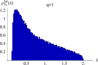
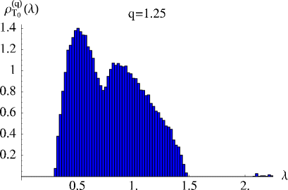
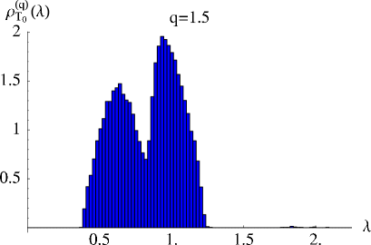
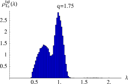
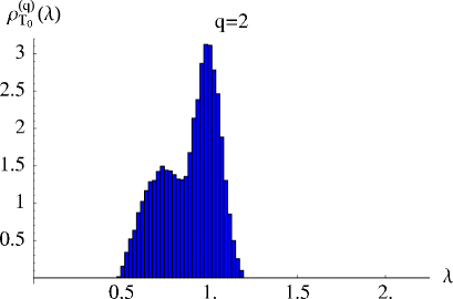
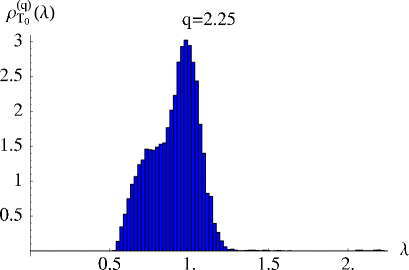
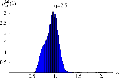
Figure 3: Spectral densities $\rho_{T_{0}}^{(q)}(\lambda)$ of the power mapped correlation matrices $C^{(q)}$. The length of the time series is always $T_{0}=1650$. The values of the powers used are $q=1.0,1.25,1.5,1.75,2.0,2.25,2.5$. An ensemble of 25 matrices $C$ was simulated which were power mapped onto $C^{(q)}$. The densities are given in units of $K$.

comprises all elements outside the blocks, where $k\neq l$ and $b(k)\neq b(l)$, we find that, for $q>1$, the power mapped matrix $C^{(q)}(T)$ is block diagonal to leading order $1/\sqrt{T}$. This explains why the power mapping has an effect which is comparable to a prolongation of the time series. At first sight, one would expect that the effect is the stronger, the larger the value of $q$. However, this is not so, because the $T$ independent terms are different for the matrix elements in the blocks: in the first case (23) of the diagonal elements, it is unity, but a number smaller than unity in the second case (24). The larger the value of $q$, the smaller becomes the latter term. Hence, the unity in the diagonal elements dominates more and more, driving the eigenvalues towards unity. The effect discussed above which is comparable to a prolongation of the time series, leads to the separation of the spectral densities into two peaks. If $q$ becomes too large, this is counteracted, and the two peaks merge again. Consequently, there must be an optimal values for $q$. In the numerical simulation we found that it is roughly $q=1.5$.

For infinitely long time series $T\to\infty$, the power mapped correlation matrix $C^{(q)}(\infty)$ is trivially block diagonal. The eigenvalues $\lambda_{k}^{(q)}(\infty)$ and the spectral density $\rho_{\infty}^{(q)}(\lambda)$ are found along lines similar to the ones leading to Eq. (12). We arrive at

$$\rho_{\infty}^{(q)}(\lambda) = \sum_{b=1}^{B}(\kappa_{b}-1)\delta\left(\lambda-\left(1-\left(\frac{p_{b}}{1+p_{b}}\right)^{q}\right)\right)$$ (26)

$$+\sum_{b=1}^{B}\delta\left(\lambda-\left(1+(\kappa_{b}-1)\left(\frac{p_{b}}{1+p_{b}}\right)^{q}\right)\right)+\kappa\delta\left(\lambda-1\right)\ .$$

This correctly reduces to Eq. (12) for $q=1$. As already argued, the peaks due to the first term move towards the peak due to the third term if $q$ is made large. Again, the $\delta$ peaks are smeared out if the length of the time series is finite. We show in C that the noisy spectral density $\rho_{T}^{(q)}(\lambda)$ of the power mapped correlation matrix can be estimated by

$$\rho_{T}^{(q)}(\lambda) = (K-\kappa-B)G(\lambda-\mu_{B}^{(q)},(v_{B}^{(q)})^{2}/T)$$ (27)

$$+\sum_{b=1}^{B}\delta\left(\lambda-\left(1+(\kappa_{b}-1)\left(\frac{p_{b}}{1+p_{b}}\right)^{q}\right)\right)$$

$$+\kappa G(\lambda-1,(v_{0}^{(q)})^{2}/T^{q})\ .$$

Here, the parameters $(v_{B}^{(q)})^{2}$ and $(v_{0}^{(q)})^{2}$ collect the effects due to the smearing out and

$$\mu_{B}^{(q)}=\frac{1}{B}\sum_{b=1}^{B}\left(1-\left(\frac{p_{b}}{1+p_{b}}\right)^{q}\right)=1-\frac{1}{B}\sum_{b=1}^{B}\left(\frac{p_{b}}{1+p_{b}}\right)^{q}$$ (28)

approximates the center of the Gaussian due the true correlations in the first term of Eq. (27). The third term estimates the peaks due to the noise. As discussed in C, these two contributions are affected differently as finite lengths of the time series are concerned. Thus, it is useful to scale the variance with $1/T$ in the first term, but with $1/T^{q}$ in the third one.

4.3 Detecting Different Correlation Structures

We consider three examples for different correlation structures. The parameters are listed in table 2, and the corresponding correlation matrices $C$ are displayed in figure 4. We refer to the three examples as top, middle and bottom structure, respectively.

Table 2: The sizes $\kappa_{b}$ and the weights $p_{b}$ for the industrial branches used in the numerical simulation for the three ensembles of correlation matrices with different structures. The total dimension of the matrices is always $K=508$.

• Top structure: the number of industrial branches is $B=11$, $\kappa=76$ companies are in no branch.

• $b$	1	2	3	4	5	6	7	8	9	10	11
  $\kappa_{b}$	2	4	7	10	15	20	30	42	64	98	140
  $p_{b}$	0.5	0.75	0.85	0.9	0.93	0.95	0.96	0.97	0.984	0.989	0.99

• Middle structure: the number of industrial branches is $B=6$, $\kappa=256$ companies are in no branch.

• $b$	1	2	3	4	5	6
  $\kappa_{b}$	4	8	16	32	64	128
  $p_{b}$	0.008	0.01	0.03	0.07	0.2	0.99

• Bottom structure: the number of industrial branches is $B=2$, $\kappa=400$ companies are in no branch.

• $b$	1	2
  $\kappa_{b}$	4	104
  $p_{b}$	0.75	0.99

For all three structures, the total number of companies is $K=508$ and the length of the time series is $T_{0}=1650$. The top structure has many branches ($B=11$) with relatively strong correlations and little noise, the middle structure has less branches ($B=6$) with weaker correlations and more noise and, finally, the bottom structure has only $B=2$ branches with stronger correlations, and a considerable amount of noise. We notice that the weights $p_{b}$ are not chosen according to Eq. (11). Rather, we adjusted them in such a way that the spectral densities $\rho_{T_{0}}(\lambda)$ for the middle and the bottom structure look as similar as possible. This can be seen in the left column of figure 5. The top structure serves as a reference example. As the figure shows, the true correlations are so dominating that the spectral density is already almost separated in two substructures which are separated by a kink around $\lambda=1$. Thus, the top structure is an idealizing example.

We now apply the power mapping and calculate matrices $C^{(q)}$ according to Eq. (22). We choose the value $q=1.5$ which we identified as optimal in Sec. 4.1. The resulting spectral densities $\rho_{T_{0}}^{(q)}(\lambda)$ are shown in the right column of figure 5. For each of the three structures, we see the separation into two peaks, the left one corresponding to the true correlations, the right one to the noise. As expected, the spectral density for the top structure consisting of a big left peak and a small right peak differs considerably from the ones for the middle and the bottom structures where the left peaks are small and the right peaks big. This nicely confirms our expectation that the power mapping is capable of efficiently distinguishing the gross structures in the correlation matrices.

• 

• 

• 

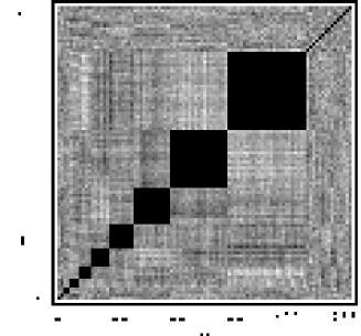
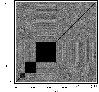
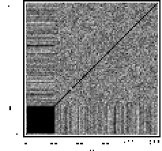
Figure 4: Three correlation matrices $C$ with different correlation structure. The parameters for the top, the middle and the bottom structure, respectively, are given in table 2. The amount of noise in the middle and the bottom structure is much higher than in the top structure.

It is now interesting to compare the spectral densities for the middle and the bottom structure: although the shape of densities $\rho_{T_{0}}(\lambda)$ in the left column of figure 5 can hardly be distinguished, the densities $\rho_{T_{0}}^{(q)}(\lambda)$ for the power mapped correlation matrices, shown in the right column, have similar, but distinguishable shapes. For both structures, the left peak is small, the right one big. However, for the bottom structure, the right peak is narrower and its left shoulder is steeper. Hence, the power mapping also gives useful information about the fine structure in the correlation matrices.

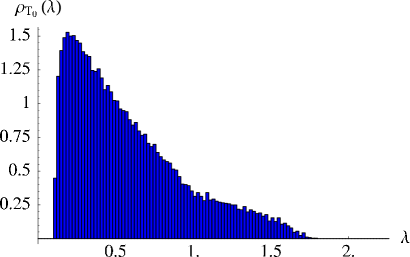
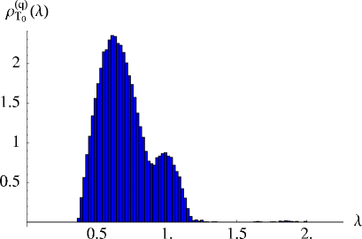
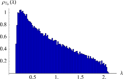
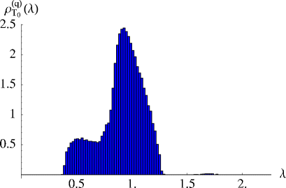
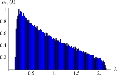
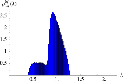
Figure 5: Left column: Spectral densities $\rho_{T_{0}}(\lambda)$ of the original correlation matrices $C$. Right column: Spectral densities $\rho_{T_{0}}^{(q)}(\lambda)$ of the same, but power mapped correlation matrices $C^{(q)}$. The length of the time series is always $T_{0}=1650$. An ensemble of 25 matrices $C$ was simulated for each structure. The value of the power used is always $q=1.5$. The 25 matrices $C$ which were simulated for each structure were individually power mapped onto matrices $C^{(q)}$, forming a new ensemble for each structure. The densities are given in units of $K$.

4.4 Measuring Correlations and Noise

Using the estimate (27), we can obtain some further understanding of why $q=1.5$ is a good value for the power mapping. The two Gaussian peaks which emerge from the power mapping, i.e. the one due to the true correlations and the one due to the noise, are separated if there is some space between the left side of the former and the right side of the latter. According to Eq. (27), the peaks should be separated if we have

$$1-\frac{v_{0}^{(q)}}{T^{q/2}}>\mu_{B}^{(q)}+\frac{v_{B}^{(q)}}{\sqrt{T}}\ ,$$ (29)

or, equivalently, if the function

$$H(q,T)=\frac{1}{B}\sum_{b=1}^{B}\left(\frac{p_{b}}{1+p_{b}}\right)^{q}-\frac{v_{0}^{(q)}}{T^{q/2}}-\frac{v_{B}^{(q)}}{\sqrt{T}}$$ (30)

is positive. Here, we used Eq. (28). In figure 6, we display the function $H(q,T)$ for different power mapped correlation matrices starting from the original one used in Sec. 3.1 with $T=T_{0}=1650$. Obviously, we may define the optimal $q$ value as the point where $H(q,T_{0})$ reaches its maximum which is given by the equation $\partial H(q,T_{0})/\partial q=0$. Indeed, this value is close to $q=1.5$. The parameters $v_{0}^{(q)}$ and $v_{B}^{(q)}$ used in figure 6 were obtained from the fitting procedure to be described in the following. As the dependence of $H(q,T)$ on $q$ is very complicated, we do not go into a further analytical discussion.

• 

Figure 6: A typical example for the function $H(q,T)$ versus the power $q$. The parameters for the original correlation matrix in Sec. 3.1 are used with $T=T_{0}=1650$. The optimal $q$ value is defined by the maximum value of $H(q,T_{0})$ which is seen to be reached near $q=1.5$.

To fit the spectral density of the power mapped correlation matrices, we use an ansatz motivated by the estimate (27). As we only want to fit the bulk part, we ignore the second term in the estimate (27) due to the large eigenvalues and take

$$\rho_{\rm bulk}^{(q)}(\lambda)=R_{B}^{(q)}G(\lambda-\mu_{B}^{(q)},(\sigma_{B}^{(q)})^{2})+R_{0}^{(q)}G(\lambda-1,(\sigma_{0}^{(q)})^{2})\ .$$ (31)

The prefactors $R_{B}^{(q)}$, $R_{0}^{(q)}$, the standard deviations $\sigma_{B}^{(q)}$, $\sigma_{0}^{(q)}$ and the mean value $\mu_{B}^{(q)}$ are fit parameters. This relatively high number of fit parameters is acceptable, because the data to be fitted have a clear structure. Moreover, it should be emphasized that we are only interested in obtaining proper estimates by these fits. From the previous discussion, we expect that the fit should approximately give, first, $R_{B}^{(q)}=K-\kappa-B$ and $R_{0}^{(q)}=\kappa$ for the prefactors and, second, the scaling behavior $(\sigma_{B}^{(q)})^{2}=(v_{B}^{(q)})^{2}/T$ and $(\sigma_{0}^{(q)})^{2}=(v_{0}^{(q)})^{2}/T^{q}$ for the variances. We employ the parameters $\sigma_{B}^{(q)}$ and $\sigma_{0}^{(q)}$ instead of the parameters $v_{B}^{(q)}$ and $v_{0}^{(q)}$, because, in practice, one will mostly have to deal with correlation matrices for one fixed length $T$ of the time series. As an example, we fit the ansatz (31) to the spectral density of the power mapped correlation matrix discussed in Sec. 4.1 for $q=1.5$. The result is shown in figure 7.

• 

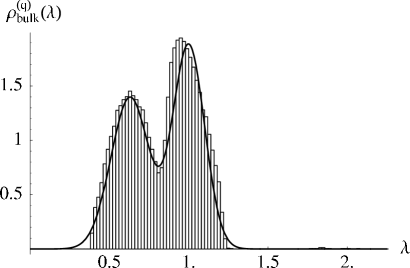
Figure 7: Fit of the ansatz (31) to the bulk part of the spectral density for the power mapped correlation matrix used in Sec. 4.1 with $q=1.5$. The density is given in units of $K$.

We obtain for the prefactors $R_{B}^{(q)}=0.42K=213$, $R_{0}^{(q)}=0.47K=239$, for the standard deviations $\sigma_{B}^{(q)}=0.12$, $\sigma_{0}^{(q)}=0.10$ and for the mean value $\mu_{B}^{(q)}=0.63$. Thus, we obtain the estimate $\kappa=R_{0}^{(q)}=239$ for the number of companies which are not in any branch. This is in fair agreement with the true value $\kappa=256$. The sum $R_{B}^{(q)}+R_{0}^{(q)}=0.89K=452$ deviates by about ten percent from the theoretical value $R_{B}^{(q)}+R_{0}^{(q)}=K-B=502$. This is not so surprising, considering the fact that our ansatz (31) can only be a rough approximation. Hence, we suggest to use the ratio

$$r^{(q)}=\frac{R_{0}^{(q)}}{R_{B}^{(q)}}$$ (32)

to characterize a correlation matrix. The larger $r^{(q)}$, the more noise is present, the smaller $r^{(q)}$, the stronger are the true correlations. In our example, we have $r^{(q)}=1.12$, implying that noise and true correlations are more or less equally strong. Advantageously, the ratio (32) is not so sensitive to the total number $K$ of companies, implying that correlation matrices of different sizes $K$ can have the same $r^{(q)}$. Of course, the number $K$, the dimension of the correlation matrix, is always known in an analysis. In the previous Sec. 4.3, we discussed a correlation matrix, labeled “middle structure”, also involving $\kappa=256$ companies which are in no branch. Most of the correlations within the branches are so weak that the left peak in the middle of the right column in figure 5 is considerably smaller than the one in figure 7. The ratio $r^{(q)}$ makes the desired distinction: the overall strength of the true correlations is much weaker than in the present case. In addition, the standard deviation $\sigma_{B}^{(q)}$ and the mean value $\mu_{B}^{(q)}$ yield information about the spreading of the weights $p_{b}$ and about their average.

Finally, we test the quality of the scaling behavior $\sigma_{B}^{(q)}\propto 1/\sqrt{T}$ and $\sigma_{0}^{(q)}\propto 1/T^{q/2}$ for the standard deviations. To this end, we generate correlation matrices for various lengths $T$ of the time series and power map them using $q=1.0$, $q=1.25$ and $q=1.5$. We fit the resulting spectral densities using the ansatz (31), extract the standard deviations $\sigma_{B}^{(q)}$ and $\sigma_{0}^{(q)}$, and fit the latter to the expected scaling behavior $1/\sqrt{T}$ and $1/T^{q/2}$, respectively. The expectation is well confirmed for $\sigma_{B}^{(q)}$. In the case of $\sigma_{0}^{(q)}$, the general trend is reproduced for the three $q$ values. For $q=1.5$, however, the most interesting value, the agreement is good. This is encouraging, because the steps that led to the estimate (27) involved various approximations. In any case, as already argued, the practical applicability of our ansatz (31) is not affected by these scaling questions.

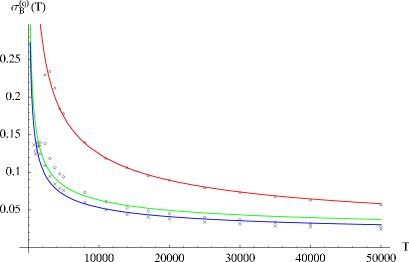
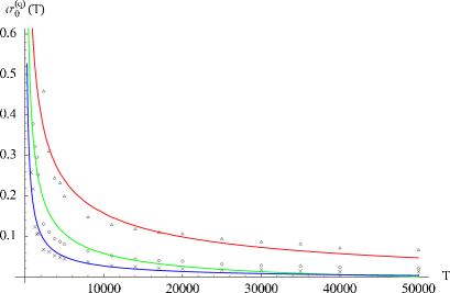
Figure 8: Standard deviations $\sigma_{B}^{(q)}$ (top part) and $\sigma_{0}^{(q)}$ (bottom part) versus the length $T$ of the time series. The dots are the data points obtained from the fits to the spectral densities. The solid lines are the fits of the expected scaling behavior $1/\sqrt{T}$ and $1/T^{q/2}$ to these data points. The top, middle and bottom curves correspond to $q=1.0$, $q=1.25$ and $q=1.5$, respectively.

As figure 8 shows, both standard deviations $\sigma_{B}^{(q)}$ and $\sigma_{0}^{(q)}$ become smaller as $q$ is made larger while $T$ is kept fixed. This is why the power mapping can be viewed as effectively prolonging the time series: To obtain given values for the standard deviations, one can either keep $q=1$ and make the time series longer or make $q$ larger and leave $T$ unchanged. For example, compared to the correlation matrix with $T=1000$ and $q=1$, the noise is reduced by 60% when one goes to $T=10000$ without changing $q=1$ and it is reduced by 75% when one applies the power mapping with $q=1.5$ while keeping $T=1000$. This is most important for applications, because time series for stocks with $T=10000$, say, are seldom available, while time series with $T=1000$ are easily accessible. Thus, power mapping can lead to better estimates for the risk and for related quantities such as the Value–at–Risk [2, 3].

5 Summary and Conclusion

We developed a new method to identify and estimate the noise and, hence, also the strength of the true correlations in a financial correlation matrix. The essence of our approach is the power mapping. It suppresses those matrix elements which can be associated with the noise. Our approach could be seen as an generalization and extension of shrinking techniques [28] used in contexts different from the present one. Importantly, the spectral density changes drastically due to the suppression. The method itself yields a criterion to choose the optimal power. Loosely speaking, our method can be interpreted as an effective prolongation of the time series. This feature makes it particularly suited for problems in which, for whatever reason, only relatively short time series are available. We expect that our approach, which is new to the best of our knowledge, can also be useful in other time series problems. Although we presented our method in the framework of stocks, we emphasize that it is applicable to every correlation matrix of time series, independent of what these time series describe: in the context of finance, these can be stocks, interest rates, exchange rates or other risk factors, or, in other fields of science, completely different observables. Moreover, advantageously, our approach does not involve further data processing or any other additional input.

Since our method does not use the large eigenvalues due to the branches, it is a fundamentally different alternative to the technique of Gopikrishnan et al. [10] which is based on such information. Our method automatically takes into account all branches, because all of them will contribute to the bulk of the spectral density. Thus, even if a large eigenvalue is not large enough to lie outside the bulk, our method will not miss the contribution of the corresponding branch. We also demonstrated, how the power mapping allows one to distinguish different correlation structures.

Further work is in progress, in particular applications to empirical correlation matrices obtained from real market data.

Appendix A Normalizations and Features of Correlation Matrices

Empirical correlation matrices for the time series $S_{k}(t),\ k=1,\ldots,K$ of stocks, say, are often constructed in the following way: to remove the drift in the data, one, first, takes the logarithms and, second, normalizes the resulting time series $G_{k}(t),\ k=1,\ldots,K$ to zero mean and unit standard deviation,

$$M_{k}(t)=\frac{G_{k}(t)-\langle G_{k}(t)\rangle_{T}}{\sqrt{\langle G_{k}^{2}(t)\rangle_{T}-\langle G_{k}(t)\rangle_{T}^{2}}}\ .$$ (33)

By construction, we have $\langle M_{k}(t)\rangle_{T}=1$, independently of how the averaging procedure is defined and for all $T$. We notice that this is not the case for our model in Eq. (3). Using this normalization, the correlation matrix is given by

$$C_{kl}(T) = \langle M_{k}(t)M_{l}(t)\rangle_{T}$$ (34)

$$= \frac{\langle G_{k}(t)G_{l}(t)\rangle_{T}-\langle G_{k}(t)\rangle_{T}\langle G_{l}(t)\rangle_{T}}{\sqrt{\langle G_{k}^{2}(t)\rangle_{T}-\langle G_{k}(t)\rangle_{T}^{2}}\sqrt{\langle G_{l}^{2}(t)\rangle_{T}-\langle G_{l}(t)\rangle_{T}^{2}}}\ .$$

Again, by construction, the diagonal elements are unity, $C_{kk}(T)=1$, independent of the averaging procedure chosen and also for all $T$. Once more, this differs from the diagonal elements of the correlation matrix in our model, as can be seen from Eq. (10) for $k=l$.

We now investigate the off–diagonal matrix elements for $k\neq l$. To leading order in the length $T$ of the time series, we assume

$$\langle G_{k}(t)\rangle_{T} = g_{k}+\frac{f_{k}}{\sqrt{T}}$$

$$\langle G_{k}(t)G_{l}(t)\rangle_{T} = \beta_{kl}+\frac{\gamma_{kl}}{\sqrt{T}}\ ,$$ (35)

where $g_{k}$, $f_{k}$ and $\beta_{kl}$, $\gamma_{kl}$ are constants. A straightforward calculation then yields

$$C_{kl}(T) = \frac{1}{\sqrt{\beta_{kk}-g_{k}^{2}}\sqrt{\beta_{ll}-g_{l}^{2}}}\left(c_{kl}^{(0)}+\frac{c_{kl}^{(1)}}{\sqrt{T}}\right)$$

$$c_{kl}^{(0)} = \beta_{kl}-g_{k}g_{l}$$

$$c_{kl}^{(1)} = \gamma_{kl}-g_{k}f_{l}-g_{l}f_{k}-\frac{1}{2}\left(\beta_{kl}-g_{k}g_{l}\right)$$ (36)

$$\qquad\left(\frac{\gamma_{kk}-2g_{k}f_{k}}{\beta_{kk}-g_{k}^{2}}+\frac{\gamma_{ll}-2g_{l}f_{l}}{\beta_{ll}-g_{l}^{2}}\right)$$

to leading order in $T$. We assume that the variances for infinite $T$ are non–zero, i.e. $\beta_{kk}-g_{k}^{2}>0$. As required, we have $C_{kk}(T)=1$. For $k\neq l$, the forms of the expansions to leading order in Eqs. (10) and (36) coincide. In the present discussion, we have not explicitly incorporated a structure due to branches. Such information would appear, for example, in the parameters $\beta_{kl}$.

As compared to the correlation matrices resulting from the model in Eq. (3), the difference in the normalization of the diagonal elements in Eq. (34) has only a marginal and negligible influence on the eigenvalues and the spectral density, because there are many more off–diagonal matrix elements than diagonal ones. This is also clearly borne out in Noh’s [19] and in our numerical results. Moreover, there is no structural difference for the off–diagonal matrix elements. Hence, we are convinced that the results of the present work carry over to models involving a normalization of the kind (33). Our main reason to work with the normalization in Noh’s model is the fact that the limiting case for infinitely long time series $T\to\infty$ can conveniently be handled analytically.

We mention in passing that practitioners in banks and investment companies commonly work with time series having a typical length of 250 days. These time series are often exponentially weighted before the analysis. We do not employ such a weighting procedure, because we are interested in the question, how a information about correlations of longer time series can, to some extent and under proper conditions, be estimated from shorter time series.

Furthermore, a comment regarding the branches in the model is in order. An international portfolio is likely to contain globally operating, large companies. Their activities directly affect various branches, but they are also under different economical influences in different countries. In such cases, it is common to add a further label ”country” to the label ”branch”, denoted $b$ in our case. Generally speaking, it is often necessary to go from a one–factor model of the type discussed in the present article to a two–factor or multi–factor model. From the viewpoint of a simulation, this refined correlation structure implies the need for precise information about the weights which generalize our $p_{b}$. On the other hand, not much changes from the viewpoint of data analysis, which was the main motivation of the present work.

Appendix B Noisy Spectral Density before Power Mapping

In general, the spectral density $\rho_{T}(\lambda)$ for a given length $T$ of the time series can be written as the spectral average of the joint probability density function $P_{T}(\lambda(T))$ for the eigenvalues $\lambda_{k}(T),\ k=1,\ldots,K$ of the correlation matrix $C(T)$,

$$\rho_{T}(\lambda)=\int d[\lambda(T)]P_{T}(\lambda(T))\sum_{k=1}^{K}\delta\left(\lambda-\lambda_{k}(T)\right)\ ,$$ (37)

where $d[\lambda(T)]$ stands for the product of all differentials $d\lambda_{k}(T)$. In our notation, we distinguish the argument $\lambda$ of the density and the eigenvalues $\lambda_{k}(T)$ of the correlation matrix which are always written with their argument $T$. In particular, Eq. (37) is also valid for $T\to\infty$ and we have

$$\rho_{\infty}(\lambda)=\int d[\lambda(\infty)]P_{\infty}(\lambda(\infty))\sum_{k=1}^{K}\delta\left(\lambda-\lambda_{k}(\infty)\right)\ .$$ (38)

As a consequence of Eq. (13), the joint probability densities for finite and infinite $T$ can, to leading order $1/\sqrt{T}$, be related according to

$$P_{T}(\lambda(T)) = \int d[\lambda(\infty)]P_{\infty}(\lambda(\infty))\int d[a]\prod_{l=1}^{K}G(a_{l},1)$$ (39)

$$\quad\prod_{k=1}^{K}\delta\left(\lambda_{k}(T)-\lambda_{k}(\infty)-\frac{v_{k}}{\sqrt{T}}a_{k}\right)$$

$$= \int d[\lambda(\infty)]P_{\infty}(\lambda(\infty))$$

$$\quad\prod_{k=1}^{K}G(\lambda_{k}(T)-\lambda_{k}(\infty),v_{k}^{2}/T)\ .$$

Here, $G(z,w^{2})$ is the Gaussian depending on the variable $z$, centered at zero, with variance $w^{2}$. We plug Eq. (39) into Eq. (37), do the integrals over $\lambda(T)$ and find

$$\rho_{T}(\lambda) = \int d[\lambda(\infty)]P_{\infty}(\lambda(\infty))\sum_{k=1}^{K}G(\lambda-\lambda_{k}(\infty),v_{k}^{2}/T)$$ (40)

$$= \sum_{k=1}^{K}\int_{-\infty}^{+\infty}d\lambda^{\prime}G(\lambda^{\prime}-\lambda,v_{k}^{2}/T)$$

$$\quad\int d[\lambda(\infty)]P_{\infty}(\lambda(\infty))\delta\left(\lambda^{\prime}-\lambda_{k}(\infty)\right)\ .$$

In the second step, we inserted the integration over $\lambda^{\prime}$ using a $\delta$ function. Since we may assume that the joint probability density $P_{T}(\lambda(\infty))$ is invariant under the exchange of its arguments $\lambda_{k}(\infty)$, we can employ Eq. (38) and integrate over the eigenvalues. We arrive at

$$\rho_{T}(\lambda)=\int_{-\infty}^{+\infty}\overline{G}_{T}(\lambda^{\prime}-\lambda,v^{2})\rho_{\infty}(\lambda^{\prime})d\lambda^{\prime}\ ,$$ (41)

where we defined the average

$$\overline{G}_{T}(z,v^{2})=\frac{1}{K}\sum_{k=1}^{K}G(z,v_{k}^{2}/T)$$ (42)

over the $K$ Gaussians. The parameters $v_{k}^{2}$ are functions of the sizes $\kappa_{b}$ and the weights $p_{b}$. Thus, to leading order $1/\sqrt{T}$, we can obtain the spectral density for finite $T$ from that for infinite $T$ by convoluting the latter with a superposition of Gaussians.

Formula (41) is valid for every spectral density $\rho_{\infty}(\lambda)$. We now apply it to the spectral density (12) and obtain

$$\rho_{T}(\lambda) = \sum_{b=1}^{B}(\kappa_{b}-1)\overline{G}_{T}\left(\lambda-\frac{1}{1+p_{b}},v^{2}\right)$$ (43)

$$+\sum_{b=1}^{B}\delta\left(\lambda-\frac{1+\kappa_{b}p_{b}}{1+p_{b}}\right)+\kappa\overline{G}_{T}\left(\lambda-1,v^{2}\right)\ .$$

As the second term contains the large, widely spaced eigenvalues, we neglect the smearing out there. With this additional approximation, the result (43) is valid to leading order $1/\sqrt{T}$. It gives an analytical motivation for the estimate (21).

Appendix C Noisy Spectral Density after Power Mapping

The crucial effect of the power mapping is the preservation of the block structure in $C^{(q)}(T)$ up to order $1/\sqrt{T}$. This is evident from Eqs. (23) and (24). Only the inclusion of the order $1/T^{q/2}$ destroys this block structure as seen in Eq. (25). Hence, to understand the noisy spectral density up to order $1/\sqrt{T}$, we can apply the methods of B individually to those $\kappa_{b}\times\kappa_{b}$ blocks which contain the companies of one branch. A modification occurs for the $\kappa\times\kappa$ block collecting the companies which do not belong to a branch. According to Eq. (23), this block is up to order $1/\sqrt{T}$ still a diagonal matrix, implying that the eigenvalues equal the diagonal elements. Since we have $p_{b}=0$, they are given by $\lambda_{k}^{(q)}(T)=(C_{kk}(T))^{q}=1+qa_{kk}\sqrt{2/T}$. On the other hand, employing a line of reasoning similar to the one in Sec. 3.2, the eigenvalues of the blocks corresponding to a branch will have have the form

$$\lambda_{k}^{(q)}(T)=\lambda_{k}^{(q)}(\infty)+\frac{v_{k}^{(q)}}{\sqrt{T}}a_{k}^{(q)}$$ (44)

where $a_{k}^{(q)}$ are independent Gaussian distributed variables with zero mean and unit variance. The parameters $v_{k}^{(q)}$ result from a superposition of $\kappa_{b}$ terms of order unity. Thus, the Gaussian smearing out will be stronger, roughly by a factor $\kappa_{b}$, for the eigenvalues $\lambda_{k}^{(q)}(\infty)$ of the blocks corresponding to a branch than for the eigenvalues $\lambda_{k}^{(q)}(\infty)=1$ which do not belong to a branch. If we make the assumption that the sizes $\kappa_{b}$ are large, we can neglect the smearing out of the latter eigenvalues. We emphasize that this is an additional approximation which is not motivated by the asymptotic expansion in $T$. Under this assumption, we obtain from Eq. (26) to leading order $1/\sqrt{T}$ the estimate

$$\rho_{T}^{(q)}(\lambda) = \sum_{b=1}^{B}(\kappa_{b}-1)\overline{G}_{T}\left(\lambda-\left(1-\left(\frac{p_{b}}{1+p_{b}}\right)^{q}\right),(v^{(q)})^{2}\right)$$ (45)

$$+\sum_{b=1}^{B}\delta\left(\lambda-\left(1+(\kappa_{b}-1)\left(\frac{p_{b}}{1+p_{b}}\right)^{q}\right)\right)+\kappa\delta\left(\lambda-1\right)\ .$$

Since the second term involves the large eigenvalues outside the bulk whose spacing is large compared to the smearing out, we may assume that the corresponding $\delta$ functions are not affected, either. To find an estimate to leading order $1/T^{q/2}$, we must apply the methods of B to the entire matrix, because the block structure is destroyed. We replace Eq. (44) with

$$\lambda_{k}^{(q)}(T)=\lambda_{k}^{(q)}(\infty)+\frac{v_{k}^{(q)}}{\sqrt{T}}a_{k}^{(q)}+\frac{\widetilde{v}_{k}^{(q)}}{T^{q/2}}\widetilde{a}_{k}^{(q)}\ .$$ (46)

As we are only interested in a qualitative discussion, we make the further assumption that the $\widetilde{a}_{k}^{(q)}$ are independent Gaussian variables with zero mean and unit variance. The smearing out to order $1/T^{q/2}$ will not affect the first term of Eq. (45), because it is already of order $1/\sqrt{T}$. However, we cannot neglect it in the third term, because the parameters $\widetilde{v}_{k}^{(q)}$ are now of order $K$. We obtain

$$\rho_{T}^{(q)}(\lambda) = \sum_{b=1}^{B}(\kappa_{b}-1)\overline{G}_{T}\left(\lambda-\left(1-\left(\frac{p_{b}}{1+p_{b}}\right)^{q}\right),(v^{(q)})^{2}\right)$$ (47)

$$+\sum_{b=1}^{B}\delta\left(\lambda-\left(1+(\kappa_{b}-1)\left(\frac{p_{b}}{1+p_{b}}\right)^{q}\right)\right)$$

$$+\kappa\overline{G}_{T^{q}}\left(\lambda-1,(\widetilde{v}^{(q)})^{2}\right)\ .$$

Replacing each of the sums over the functions $\overline{G}_{T}$ and $\overline{G}_{T^{q}}$ with one Gaussian, we arrive at the estimate (27).

References

References

- [1] E.J. Elton and M.J. Gruber, Modern Portfolio Theory and Investment Analysis (J. Wiley, New York 1995).
- [2] R. Eller and H.P. Deutsch, Derivate und Interne Modelle, Modernes Risikomanagement (Schäffer-Pöschel Verlag, Stuttgart 1998).
- [3] J. Longerstaey, A. Zangari and S. Howard, Risk -Technical Document (J. P. Morgan, New York 1996).
- [4] L. Laloux, P. Cizeau, J.P. Bouchaud and M. Potters Phys. Rev. Lett. 83, 1467 (1999).
- [5] V. Plerou, P. Gopikrishnan, B. Rosenow, L.A.N. Amaral and H.E. Stanley, Phys. Rev. Lett. 83, 1471 (1999).
- [6] M.L. Mehta, Random Matrices, 2nd edition, (Academic Press, San Diego 1990).
- [7] F. Haake, Quantum Signatures of Chaos, 2nd edition, (Springer Verlag, Berlin 2001).
- [8] T. Guhr, A. Müller–Groeling and H.A. Weidenmüller, Phys. Rep. 299, 189 (1998).
- [9] Z. Burda, J. Jurkiewicz, M.A. Nowak, G. Papp and I. Zahed, cond-mat/0103108; cond-mat/0103108.
- [10] P. Gopikrishnan, B. Rosenow, V. Plerou, L.A.N. Amaral and H.E. Stanley, cond-mat/0011145.
- [11] V. Plerou, P. Gopikrishnan, B. Rosenow, L.A.N. Amaral, T. Guhr and H.E. Stanley, cond-mat/0108023.
- [12] R.N. Mantegna, Eur. Phys. J. B11, 193 (1999).
- [13] R.N. Mantegna and H.E. Stanley, An Introduction to Econophysics (Cambridge University Press, Cambridge, 2000)
- [14] J.P. Bouchaud and M. Potters, Theory of Financial Risks (Cambridge University Press, Cambridge, 2000)
- [15] J. Voit, The Statistical Mechanics of Financial Markets (Springer, Heidelberg, 2001)
- [16] W. Paul and J. Baschnagel, Stochastic Processes: From Physics to Finance (Springer, Berlin, 1999)
- [17] P. Gopikrishnan, V. Plerou, L.A. Amaral, M. Meyer and H.E. Stanley, Phys. Rev. E60, 5305 (1999).
- [18] P. Gopikrishnan, V. Plerou, L.A. Amaral, M. Meyer and H.E. Stanley, Phys. Rev. E60, 6519 (1999).
- [19] J.D. Noh, Phys. Rev. E61, 5981 (2000), cond-mat/9912076.
- [20] S. Ross, J. Econ. Theory 13, 341 (1976).
- [21] M. Marsili, cond-mat/0003241.
- [22] L. Kullmann, J. Kertész and R.N. Mantegna, cond-mat/0002238.
- [23] F.Y. Wu, Rev. Mod. Phys. 54, 235 (1982).
- [24] U. Krengel, Einführung in die Wahrscheinlichkeitstheorie und Statistik (Vieweg, Braunschweig 1991).
- [25] J.J.M. Verbaarschot and T. Wettig, Ann. Rev. Nucl. Part. Sci. 50 (2000) 343; hep-ph/0003017.
- [26] F.J. Dyson, Revista Mexicana de Física 20, 231 (1971).
- [27] A.M. Sengupta and P.P. Mitra, cond-mat/9709283.
- [28] R. Dahlhaus, private communication, Oberwolfach, 2002.