Enhancement by polydispersity of the biaxial nematic phase
in a mixture of hard rods and plates

Abstract

The phase diagram of a polydisperse mixture of uniaxial rod-like and plate-like hard parallelepipeds is determined for aspect ratios $\kappa=5$ and 15. All particles have equal volume and polydispersity is introduced in a highly symmetric way. The corresponding binary mixture is known to have a biaxial phase for $\kappa=15$, but to be unstable against demixing into two uniaxial nematics for $\kappa=5$. We find that the phase diagram for $\kappa=15$ is qualitatively similar to that of the binary mixture, regardless the amount of polydispersity, while for $\kappa=5$ a sufficient amount of polydispersity stabilizes the biaxial phase. This provides some clues for the design of an experiment in which this long searched biaxial phase could be observed.

Systems of anisotropic molecules with two symmetry axes may form a biaxial nematic phase. In this phase molecules align preferentially along two perpendicular axes. The biaxial phase is experimentally difficult to observe because in systems with biaxial molecules it is preempted by smectic or solid phases. This led Alben Alben (1973) to propose an alternative system which should behave similarly, but in which spatial ordering is difficulted: a mixture of hard rods and plates. His analysis of this system with a mean-field lattice model showed a phase diagram with four phases: isotropic fluid (I), rod-like nematic (N⁺), plate-like nematic (N^-), and biaxial (B). The latter separates the two nematics with second-order transition lines when composition is varied from rod-rich to plate-rich. Upon increasing concentration, for a rod-rich (plate-rich) composition the system first undergoes a first-order I–N⁺ (I–N^-) transition and then a second order N⁺–B (N^-–B) transition. At the crossover there is simply a continuous I–B transition. Two continuous and two first-order transitions meet at this multicritical point. At the conclusions of his work, Alben mentions that a N⁺–N^- phase separation might replace the B phase, but does not considers this possibility in his analysis. A similar phase behavior has later been obtained by other authors using different models Rabin et al. (1982); Stroobants and Lekkerkerker (1984); Sokolova and Vlasov (1997); Chrzanowska (1997). They take into account the effect of having free (rather than restricted to a lattice) rotations and/or translations. From them one learns three main things: first of all, that Alben’s phase diagram is qualitatively correct; secondly, that there is a symmetric mixture, namely that with rods and plates having the same molecular volume (hence parallel or perpendicular like particles have the same excluded volume), for which the multicritical point appears more or less at equimolar composition; and thirdly, that the phase diagram is perfectly symmetric about equimolarity only if virial coefficients higher than the second are neglected.

The first experimental observation of a B phase was obtained by Yu and Saupe Yu and Saupe (1980) in a ternary lyotropic mixture of potassium laureate, 1–decanol and water. This system forms lamellar and cylindrical micelles. By varying composition and concentration N^± and B phases appear, in a configuration that reproduces Alben’s phase diagram around the multicritical point. Although this was first considered an experimental realization of Alben’s model, it was latter recognized that micelles can really change shape from rod-like to plate-like through biaxial forms as we move in the phase diagram. A Landau theory for a system of shape-changing micelles Tolédano and Neto (1994) does in fact reproduce even the most peculiar features of Yu-Saupe’s system (like reentrance in the isotropic phase upon increasing concentration). So the experimental observation of the B phase in a mixture of rods and plates remains a open problem.

At the same time van Roij and Mulder van Roij and Mulder (1994) introduced an new important element in play. They considered the rod-plate mixture version of Zwanzig’s model (uniaxial parallelepipeds), as well as an expansion of the free energy up to the second virial coefficient. Then they reanalysed the phase diagram with respect to N⁺–N^- demixing for the symmetric mixture, for which the excluded volume between unlike particles is minimum (hence phase separation is least favored). What they found is that N⁺–N^- phase separation is more stable than the B phase up to aspect ratios (long-to-short axis ratio) $\kappa\approx 8.8$. Above that threshold the phase diagram is like that predicted by Alben up to a certain concentration, where phase separation again replaces the B phase. The window of stability of the B phase is relatively narrow. The driving mechanism behind this phase behavior is the larger excluded volume between unlike particles in the B phase as compared to that between like particles (the rod-plate excluded volume divided by the rod-rod one scales as $\kappa^{2/3}$ for large aspect ratios $\kappa$ van Roij and Mulder (1994)). When the gain in free volume compensates the loss in mixing entropy (and this strongly depends on concentration and composition) phase separation occurs. This phase behavior was later confirmed in simulations of symmetric mixtures of prolate and oblate ellipsoids Camp et al. (1997), the only difference being the logical asymmetry in the phase diagram of the latter (an important difference, though, because it gives rise to N^-–B coexistence).

There is a new recent experiment, this time performed on a true colloidal rod-plate mixture van der Kooij and Lekkerkerker (2000). Rod (plate) aspect ratio is $\kappa\approx 10$ (15) while plate-to-rod volume ratio is 13:1. The mixture is therefore far from being symmetric. This system shows isotropic (I) and uniaxial nematic phases, as well as biphasic (I–N^±) and triphasic (I–N⁺–N^-) coexistences, but no B phase at all (there appear more phases at higher concentrations, but they are spatially inhomogeneous Wensink et al. (2001)). This picture is consistent with the large volume difference between rods and plates, and can in fact be explained with a Parsons-Lee density functional approximation Wensink et al. (2001). This experiment introduces, however, another element of unpredicted effect on the system: polydispersity. Both rods and plates have about 20–30% polydispersity in their axis lengths. For this particular system, as theory shows Wensink et al. (2001), this does not seem to have any observable qualitative effect other than allowing for more than three phase coexistence (which is forbidden by Gibbs’s phase rule in a two-component system) at high concentrations. But as we aim to show in this letter, polydispersity has a more drastic effect in the phase behavior of the symmetric rod-plate mixture.

To this purpose, we have extended van Roij and Mulder’s model in two ways: (i) including polydispersity in a highly symmetric way, in order to minimize trivial excluded volume effects; and (ii) using fundamental-measure theory Cuesta and Martínez-Ratón (1997a, b) to model its free energy, which for homogeneous phases is equivalent to employing a $y$-expansion exact up to the third virial term (hence the phase diagram is expected to be asymmetric). Thus our system consists of a mixture of parallelepipeds of size $L\times D\times D$, all of them with equal volume: $LD^{2}=1$. If we characterize anisotropy by $L/D=\lambda$, then $L=\lambda^{2/3}$ and $D=\lambda^{-1/3}$. Rods have $1<\lambda<\infty$ while plates have $0<\lambda<1$. The composition of the mixture is then given by a (parent) probability density

$$\begin{split}p(\lambda)&=\lambda^{-1}\big{[}\zeta f(\lambda/\kappa)+(1-\zeta)f(\lambda\kappa)\big{]},\\ f(z)&=K_{0}(\alpha)^{-1}\exp[-(\alpha/2)(z^{2}+z^{-2})],\end{split}$$ (1)

where $K_{\nu}(\alpha)$ ($\alpha>0$) is the $\nu$th-order modified Bessel function, and $\kappa>1$. Function $f(z)$ is peaked around $z\approx 1$, and it is wider the smaller is $\alpha$; so $f(\lambda/\kappa)$ is peaked around $\lambda=\kappa$ and $f(\lambda\kappa)$ is peaked around $\lambda=\kappa^{-1}$. The former represents a polydisperse distribution of rods and the latter a distribution of plates, both of aspect ratio $\kappa$. Parameter $0\leq\zeta\leq 1$ allows to tune the overall composition of the mixture, since the molar fraction of the rods is given by $x_{r}(\zeta)\equiv\int_{1}^{\infty}p(\lambda)\,d\lambda$ (and that of plates by $x_{p}(\zeta)=1-x_{r}(\zeta)$, of course). The probability density $p(\lambda)$ is chosen so that if $dg(\lambda,\zeta)\equiv p(\lambda)d\lambda$, then $|dg(\lambda,\zeta)|=|dg(\lambda^{-1},1-\zeta)|$; in other words, the fraction of rods and plates within the same interval of aspect ratios are in the proportion $x_{r}(\zeta):x_{p}(1-\zeta)$. The moments of this distribution are given by $\langle\lambda^{m}\rangle=K_{m/2}(\alpha)K_{0}(\alpha)^{-1}[\zeta\kappa^{m}+(1-\zeta)\kappa^{-m}]$, explicitly showing the symmetry of the mixture.

Fundamental-measure approximation for a multicomponent mixture of hard uniaxial parallelepipeds amounts to taking for the excess (over the ideal) free energy density (in $kT$ units) Cuesta and Martínez-Ratón (1997a, b),

$$\begin{split}&\Phi=-n_{0}\ln(1-n_{3})+\frac{\sum_{\mu}n_{1}^{\mu}n_{2}^{\mu}}{1-n_{3}}+\frac{\prod_{\mu}n_{2}^{\mu}}{(1-n_{3})^{2}},\\ &\begin{array}[]{ll}\displaystyle n_{0}=\sum_{\mu,i}\rho_{i}^{\mu}\equiv\rho,&\displaystyle n_{1}^{\mu}=\sum_{i}\left[\rho D_{i}+\rho_{i}^{\mu}\left(L_{i}-D_{i}\right)\right],\\ \displaystyle n_{3}=\sum_{\mu,i}\rho_{i}^{\mu}L_{i}D_{i}^{2},&\displaystyle n_{2}^{\mu}=\sum_{i}\left[\rho L_{i}-\rho_{i}^{\mu}\left(L_{i}-D_{i}\right)\right]D_{i},\end{array}\end{split}$$

$\rho_{i}^{\mu}$ denoting the number density of parallelepipeds of species $i$ with their symmetry axes oriented along the direction $\mu(=x,y,z)$. Specializing for our system, where species are labeled by the continuous parameter $\lambda$,

$$\begin{split}\Phi&=-\rho\ln(1-\rho)+\frac{\sum_{\mu}\xi_{-}^{\mu}\xi_{+}^{\mu}}{1-\rho}+\frac{\prod_{\mu}\xi_{+}^{\mu}}{(1-\rho)^{2}},\\ \xi_{\pm}^{\mu}&\equiv\int_{0}^{\infty}\lambda^{\pm 1/3}\left[\left(\lambda^{\mp 1}-1\right)\rho^{\mu}(\lambda)+\rho(\lambda)\right]\,d\lambda,\end{split}$$ (2)

where $\rho(\lambda)=\sum_{\mu}\rho^{\mu}(\lambda)$. The total free energy density is then given by

$$\frac{\beta F}{V}=\sum_{\mu}\int_{0}^{\infty}\rho^{\mu}(\lambda)[\ln\rho^{\mu}(\lambda)-1]+\Phi$$ (3)

Details for determining phase equilibria in a system like this have been reported elsewhere Clarke et al. (2000); Sollich (2002). In brief, if at a given $\rho$ there is only one phase present, its equilibrium composition is determined by minimizing (3) with respect to $\rho^{\mu}(\lambda)$ under the constraint $\rho(\lambda)=\rho p(\lambda)$, with $p(\lambda)$ given by (1). This amounts to solving the system of equations ($\mu=x,y,z$)

$$\rho^{\mu}(\lambda)=\rho p(\lambda)\frac{e^{-\Phi^{\mu}(\lambda)}}{\sum_{\nu}e^{-\Phi^{\nu}(\lambda)}},\quad\Phi^{\mu}(\lambda)\equiv\frac{\delta\Phi}{\delta\rho^{\mu}(\lambda)}.$$ (4)

If $m>1$ phases are present in mutual equilibrium, then labeling them with $a(=1,\dots,m)$ their density distributions must verify the ‘lever rule’

$$\rho p(\lambda)=\sum_{a}v_{a}\rho_{a}(\lambda),$$ (5)

$v_{a}$ denoting the fraction of volume ocupied by the $a$th phase ($\sum_{a}v_{a}=1$). Chemical equilibrium then yields

$$\rho_{a}^{\mu}(\lambda)=\rho p(\lambda)\frac{e^{-\Phi_{a}^{\mu}(\lambda)}}{\sum_{b}v_{b}\sum_{\nu}e^{-\Phi_{b}^{\nu}(\lambda)}},$$ (6)

and this system of equations is completed by the equality of osmotic pressures between every pair of phases, where osmotic pressure is obtained from (3) as

$$\beta\Pi=\frac{\rho}{1-\rho}+\frac{\sum_{\mu}\xi_{-}^{\mu}\xi_{+}^{\mu}}{(1-\rho)^{2}}+2\,\frac{\prod_{\mu}\xi_{+}^{\mu}}{(1-\rho)^{3}}$$ (7)

First of all, as this theory has contributions of virial terms higher than the second, we have checked van Roij and Mulder’s results van Roij and Mulder (1994). So we have first chosen a bidisperse mixture (pure rods and pure plates). The resulting phase diagrams are qualitatively the same, apart from some asymmetry induced by those higher virials: for $\kappa=15$ there is a small B window bounded above by N⁺–N^- demixing, whereas no B phase appears for $\kappa=5$. In both cases, the multicritical point is found very near $x_{r}=1/2$. An important difference produced by the asymmetry is the replacement of the very narrow region of triphasic coexistence found by van Roij and Mulder by a simple N⁺–B coexistence. It is also worth mentioning that the asymmetry we obtain mirrors that of the simulations of prolate and oblate ellipsoids Camp et al. (1997) (they observe N^-–B coexistence instead). This means that the asymmetry must be strongly influenced by the details of the model (mainly the shape of the molecules and the restriction of orientations).

  

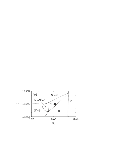
Figure 1: Phase diagram (global density, $\rho$, vs. rod molar fraction, $x_{r}$) and two details of a polydisperse rod-plate mixture with length and breadth polydispersity $\Delta_{L}=0.288$ and $\Delta_{D}=0.143$, and aspect ratio $\kappa=15$. Phases are labelled I (isotropic), N⁺ (rod-like nematic), N^- (plate-like nematic) and B (biaxial nematic). Dotted lines mark second-order phase transitions and full lines delimite coexistence regions.

We have next made the mixture polydisperse. The breadth of the two peaks in $p(\lambda)$ is controlled by $\alpha$ in (1). A quantitative characterization of the polydispersity can be given if we determine the dispersion in $L$ and $D$ as obtained from $p(\lambda)$ for $\zeta=0$ or 1. This yields

$$\Delta_{L,D}\equiv\sqrt{\frac{\langle\lambda^{2\nu/3}\rangle}{\langle\lambda^{\nu/3}\rangle^{2}}-1}=\sqrt{\frac{K_{\nu/3}(\alpha)K_{0}(\alpha)}{K_{\nu/6}(\alpha)^{2}}-1},$$ (8)

where $\nu=2$ for $\Delta_{L}$ and $\nu_{D}=1$ for $\Delta_{D}$. For $\kappa=15$ we have chosen $\alpha=1$ ($\Delta_{L}=0.288$, $\Delta_{D}=0.143$). The resulting phase diagram ($\rho$ vs. $x_{r}$) is plotted in Fig. 1. The global picture (Fig. 1a) resembles very much the bidisperse case: there are first order I–N^± transitions; the two uniaxial nematics are separated by a B phase through second order transition lines; roughly above a threshold density the latter is replaced by a wide region of N⁺–N^- coexistence; and there is a multicritical point where the two I–N^± first order transitions and the two N^±–B second order ones meet (very close to $x_{r}=1/2$). There is a difference with respect to the bidisperse phase diagram in that the lines delimiting coexistence regions do not correspond to coexisting states, but are the cloud lines (defined by points where a incipient new phase is forming) of the corresponding coexistences. For the sake of clarity, the shadow lines (density and composition of the incipient phase) are not represented. Notice that $\rho$ is the global density of the system, and does not coincide with that any of the coexisting phases (except at the cloud lines of biphasic coexistence). The details (Figs. 1b and c) show that right above the B phase there are regions of B–N^± as well as triphasic coexistence. Also remarkable are the two second-order transitions separating the B–N^± coexistence regions from the N⁺–N^- one, where upon increasing concentration the biaxial order parameter vanishes continuously, hence transforming the B phase into the second uniaxial nematic. These lines have no analogue in the bidisperse system. Finally, a global effect of polydispersity is to lower the phase diagram in densities and to make it more symmetric (probably two related effects, because the lower the density the less relevant the higher virial terms).

Figure 2: Same as Fig. 1 but for aspect ratio $\kappa=5$ and length and breath polydispersity $\Delta_{L}=0.610$ and $\Delta_{D}=0.302$.

We have checked that the region of stability of the B phase is not appreciably affected by an increase in polydispersity (using $\alpha=0.1$, i.e. $\Delta_{L}=0.610$, $\Delta_{D}=0.302$), so polydispersity does not seem to inhibit B ordering. In fact, it acts otherwise, favouring B ordering against N⁺–N^- demixing, as the case $\kappa=5$ illustrates (see Fig. 2). Again the phase diagram of this case looks very much like that of the bidisperse case if we take $\alpha=1$, i.e. no B phase appears. However, increasing polydispersity up to $\alpha=0.1$ we again obtain a region where B ordering is more stable than N⁺–N^- demixing (Fig. 2a). The B phase is limited from above by a region of B–N^- coexistence, which upon increasing density again becomes N⁺–N^- through a second order transition.

This enhancement of biaxial ordering is the most sriking effect of polydispersity. To understand why it is so we must find a mechanism by which B ordering is entropically favoured w.r.t. N⁺–N^- demixing. This mechanism is two-folded: on the one hand mixing entropy increases upon increasing polydispersity, thus penalizing demixing; but on the other hand, polydispersity increases the gain in free volume of the B phase w.r.t. that of uniaxial nematics (the average rod-plate excluded volume divided by the average rod-rod one in a perfect B phase scales as $\kappa^{2/3}e^{-c\Delta^{2}}$, $c$ being a positive constant, for large aspect ratios $\kappa$ and polydispersities in the range $1\ll\Delta_{(L,D)}\ll\sqrt{\ln\kappa}$).

This effect can be exploited in the design of an experiment to observe the B phase. The fabrication of rod-like and plate-like colloidal particles could follow similar procedures to those employed by van der Kooij and Lekkerkerker van der Kooij and Lekkerkerker (2000). Then, the mean size and polydispersity of the rods and the plates can be controlled by inducing successive fractionations (e.g. by adding a nonadsorbing polymer van der Kooij et al. (2000)), starting off from the appropriate parent distributions so as to obtain the desired final values. The key is to produce as symmetric (in particle volume) polydisperse mixtures as possible, since this seems a crucial ingredient for the stability of the B phase, with or without polydispersity. How destabilizing are the asymmetry of the mixture or the existene of a particle-volume distribution (motivated, for instance, by having independent polydispersities in length and thickness) is something that has yet to be quantified, but we expect these results to be robust against perturbations in these two directions.

A final point to be addressed is that we have not taken into account possible nonuniform phases in the determination of the phase diagram. According to the availble experiments van der Kooij and Lekkerkerker (2000) these phases appear at sufficiently high concentration, while the relevant parts of the phase diagrams we present all occur at rather low concentrations. So it seems unlikely that these parts are affected by the presence of inhomogeneous phases, but this has yet to be analyzed with some care.

This work is part of the research project BFM2000-0004 (DGI) of the Ministerio de Ciencia y Tecnología (Spain). YMR is a postdoctoral fellow of the Consejería de Educación de la Comunidad de Madrid (Spain).

References

- Alben (1973) R. Alben, J. Chem. Phys. 59, 4299 (1973).
- Rabin et al. (1982) Y. Rabin, W. E. McMullen, and W. M. Gelbart, Mol. Cryst. Liq. Cryst. 89, 67 (1982).
- Stroobants and Lekkerkerker (1984) A. Stroobants and H. N. W. Lekkerkerker, J. Phys. Chem. 88, 3669 (1984).
- Sokolova and Vlasov (1997) E. Sokolova and A. Vlasov, J. Phys.: Condens. Matter 9, 4089 (1997).
- Chrzanowska (1997) A. Chrzanowska, Phys. Rev. E 58, 3229 (1997).
- Yu and Saupe (1980) L. J. Yu and A. Saupe, Phys. Rev. Lett. 45, 1000 (1980).
- Tolédano and Neto (1994) P. Tolédano and A. M. F. Neto, Phys. Rev. Lett. 73, 2216 (1994).
- van Roij and Mulder (1994) R. van Roij and B. Mulder, J. Phys. (France) II 4, 1763 (1994).
- Camp et al. (1997) P. J. Camp, M. P. Allen, P. G. Bolhuis, and D. Frenkel, J. Chem. Phys. 106, 9270 (1997).
- van der Kooij and Lekkerkerker (2000) F. M. van der Kooij and H. N. W. Lekkerkerker, Phys. Rev. Lett. 84, 781 (2000).
- Wensink et al. (2001) H. H. Wensink, G. J. Vroege, and H. N. W. Lekkerkerker, J. Chem. Phys. 115, 7319 (2001).
- Cuesta and Martínez-Ratón (1997a) J. A. Cuesta and Y. Martínez-Ratón, Phys. Rev. Lett. 78, 3681 (1997a).
- Cuesta and Martínez-Ratón (1997b) J. A. Cuesta and Y. Martínez-Ratón, J. Chem. Phys. 107, 6379 (1997b).
- Clarke et al. (2000) N. Clarke, J. A. Cuesta, R. Sear, P. Sollich, and A. Speranza, J. Chem. Phys. 113, 5817 (2000).
- Sollich (2002) P. Sollich, J. Phys.: Condens. Matter 14, R79 (2002).
- van der Kooij et al. (2000) F. M. van der Kooij, K. Kassapidou, and H. N. W. Lekkerkerker, Nature 406, 868 (2000).