Quantum impurity solvers using a slave rotor representation

Abstract

We introduce a representation of electron operators as a product of a spin-carrying fermion and of a phase variable dual to the total charge (slave quantum rotor). Based on this representation, a new method is proposed for solving multi-orbital Anderson quantum impurity models at finite interaction strength $U$. It consists in a set of coupled integral equations for the auxiliary field Green’s functions, which can be derived from a controlled saddle-point in the limit of a large number of field components. In contrast to some finite-$U$ extensions of the non-crossing approximation, the new method provides a smooth interpolation between the atomic limit and the weak-coupling limit, and does not display violation of causality at low-frequency. We demonstrate that this impurity solver can be applied in the context of Dynamical Mean-Field Theory, at or close to half-filling. Good agreement with established results on the Mott transition is found, and large values of the orbital degeneracy can be investigated at low computational cost.

I Introduction

The Anderson quantum impurity model (AIM) and its generalizations play a key role in several recent developments in the field of strongly correlated electron systems. In single-electron devices, it has been widely used as a simplified model for the competition between the Coulomb blockade and the effect of tunnelling [1]. In a different context, the Dynamical Mean-Field Theory (DMFT) of strongly correlated electron systems replaces a spatially extended system by an Anderson impurity model with a self-consistently determined bath of conduction electrons [2, 3]. Naturally, the AIM is also essential to our understanding of local moment formation in metals, and to that of heavy-fermion materials, particularly in the mixed valence regime [4].

It is therefore important to have at our disposal quantitative tools allowing for the calculation of physical quantities associated with the AIM. The quantity of interest depends on the specific context. Many recent applications require a calculation of the localized level Green’s function (or spectral function), and possibly of some two-particle correlation functions.

Many such “impurity solvers” have been developed over the years. Broadly speaking, these methods fall in two categories: numerical algorithms which attempt at a direct solution on the computer, and analytical approximation schemes (which may also require some numerical implementation). Among the former, the Quantum Monte Carlo approach (based on the Hirsch-Fye algorithm) and the Numerical Renormalization Group play a prominent role. However, such methods become increasingly costly as the complexity of the model increases. In particular, the rapidly developing field of applications of DMFT to electronic structure calculations [5] requires methods that can handle impurity models involving orbital degeneracy. For example, materials involving f-electrons are a real challenge to DMFT calculations when using Quantum Monte Carlo. Similarly, cluster extensions of DMFT require to handle a large number of correlated local degrees of freedom. The dimension of the Hilbert space grows exponentially with the number of these local degrees of freedom, and this is a severe limitation to all methods, particularly exact diagonalization and numerical renormalization group.

The development of fast and accurate (although approximate) impurity solvers is therefore essential. In the one-orbital case, the iterated perturbation theory (IPT) approximation [6] has played a key role in the development of DMFT, particularly in elucidating the nature of the Mott transition [7]. A key reason for the success of this method is that it becomes exact both in the limit of weak interactions, and in the atomic limit. Unfortunately however, extensions of this approach to the multi-orbital case have not been as successful [8]. Another widely employed method is the non-crossing approximation, or NCA [9, 10]. This method takes the atomic limit as a starting point, and performs a self-consistent resummation of the perturbation theory in the hybridization to the conduction bath. It is thus intrinsically a strong-coupling approach, and indeed it is in the strong-coupling regime that the NCA has been most successfully applied. The NCA does suffer from some limitations however, which can become severe for some specific applications. These limitations are of two kinds:

• The low-energy behaviour of NCA integral equations is well-known to display non-Fermi liquid power laws. This can be better understood when formulating the NCA approach in terms of slave bosons [11, 12]. It becomes clear then that the NCA actually describes accurately the overscreened regime of multichannel models. This is in a sense a remarkable success of NCA, but also calls for some care when applying the NCA to Fermi-liquid systems in the screened regime. It must be noted that recent progresses have been made to improve the low-energy behaviour in the Fermi liquid case [13].

• A more important limitation for practical applications has to do with the finite-$U$ extensions of NCA equations. Standard extensions do not reproduce correctly the non-interacting $U=0$ limit. In contrast to IPT, they are not “interpolative solvers” between the weak-coupling and the strong coupling limit. Furthermore, the physical self-energy tends to develop non-causal behaviour at low-frequency (i.e. $\Sigma^{\prime\prime}_{d}(\omega)>0$) below some temperature (the “NCA pathology”) At half-filling and large $U$, this only happens at a rather low-energy scale, but away from half-filling or for smaller $U$, this scale can become comparable to the bandwith, making the finite-$U$ NCA of limited applicability.

In this article, we introduce new impurity solvers which overcome some of these difficulties. Our method is based on a rather general representation of strongly correlated electron systems, which has potential applications to lattice models as well [27]. The general idea is to introduce a new slave-particle representation of physical electron operators, which emphasizes the phase variable dual to the total charge on the impurity. This should be contrasted to slave-boson approaches to a multi-orbital AIM: there, one introduces as many auxiliary bosons as there are fermion states in the local Hilbert space. This is far from economical: when the local interaction depends on the total charge only, it should be possible to identify a collective variable which provides a minimal set of collective slave fields. We propose that the phase dual to the total charge precisely plays this role. This turns a correlated electron model (at finite $U$) into a model of spin- (and orbital-) carrying fermions coupled to a quantum rotor degree of freedom. Various types of approximations can then be made on this model. In this article, we emphasize an approximate treatment based on a sigma-model representation of the rotor degree of freedom, which is then solved in the limit of a large number of components. This results in coupled integral equations which share some similarities to those of the NCA, but do provide the following improvements:

• The non-interacting ($U=0$) limit is reproduced exactly. For a fully symmetric multi-orbital model at half-filling and in the low temperature range, the atomic limit is also captured exactly, so that the proposed impurity solver is an interpolative scheme between weak and strong coupling. The sigma-model approximation does not treat as nicely the atomic limit far from half-filling however (though improvements are possible, see section V.5).

• The physical self-energy does not display any violation of causality (even at low temperature or small $U$). This is guaranteed by the fact that our integral equations become exact in the formal limit of a large number of orbitals and components of the sigma-model field.

It should be emphasized, though, that the low-energy behaviour of our equations is similar to the (infinite-$U$) NCA, and characterized by non-Fermi liquid power laws below some low-energy scale.

As a testing ground for the new solver, we apply it in this paper to the DMFT treatment of the Mott transition in the multi-orbital Hubbard model. We find an overall very good agreement with the general aspects of this problem, as known from numerical work and from some recently derived exact results. We also compare to other impurity solvers (IPT, Exact Diagonalization, QMC, NCA), particularly regarding the one-electron spectral function.

This article is organized as follows. In section II, we introduce a representation of fermion operators in terms of the phase variable dual to the total charge (taking the finite $U$, multi-orbital Anderson impurity model as an example). In section III, a sigma-model representation of this phase variable is introduced, along with a generalization from $O(2)$ to $O(2M)$. In the limit of a large number of components, a set of coupled integral equations is derived. In section IV, we test this “dynamical slave rotor” (DSR) approach on the single-impurity Anderson model. The rest of the paper (Sec. V) is devoted to applications of this approach in the context of DMFT, which puts in perspective the advantages and limitations of the new method.

II Rotorization

The present article emphasizes the role played by the total electron charge, and its conjugate phase variable. We introduce a representation of the physical electron in terms of two auxiliary fields: a fermion field which carries spin (and orbital) degrees of freedom, and the (total) charge raising and lowering operators which we represent in terms of a phase degree of freedom. The latter plays a role similar to a slave boson: here a “slave” $O(2)$ quantum rotor is used rather than a conventional bosonic field.

II.1 Atomic model

We first explain this construction on the simple example of an atomic problem, consisting in an $N$-fold degenerate atomic level subject to a local $SU(N)$-symmetric Coulomb repulsion:

$$H_{{{\mathrm{local}}}}=\sum_{\sigma}\epsilon_{0}\,d_{\sigma}^{\dagger}d_{\sigma}+\frac{U}{2}\left[\sum_{\sigma}d_{\sigma}^{\dagger}d_{\sigma}-\frac{N}{2}\right]^{2}$$ (1)

We use here $\epsilon_{0}\equiv\epsilon_{d}+U/2$ as a convenient redefinition of the impurity level, and we recast the spin and orbital degrees of freedom into a single index $\sigma=1\ldots N$ (for $N=2$, we have a single orbital with two possible spin states $\sigma=\uparrow,\downarrow$). We note that $\epsilon_{0}$ is zero at half filling, due to particle-hole symmetry.

The crucial point is that the spectrum of the atomic hamiltonian (1) depends only on the total fermionic charge $Q=0,\cdots,N$ and has a simple quadratic dependence on $Q$:

$$E_{Q}=\epsilon_{0}Q+\frac{U}{2}\left[Q-\frac{N}{2}\right]^{2}$$ (2)

There are $2^{N}$ states, but only $N+1$ different energy levels, with degeneracies $\binom{N}{Q}$. In conventional slave boson methods [14, 15], a bosonic field is introduced for each atomic state $|\sigma_{1}\cdots\sigma_{Q}\rangle$ (along with spin-carrying auxiliary fermions $f_{\sigma}^{\dagger}$). Hence, these methods are not describing the atomic spectrum in a very economical manner.

The spectrum of (1) can actually be reproduced by introducing, besides the set of auxiliary fermions $f_{\sigma}^{\dagger}$, a single additional variable, namely the angular momentum $\hat{L}=-i\partial/\partial\theta$ associated with a quantum $O(2)$ rotor $\theta$ (i.e. an angular variable in $[0,2\pi]$. Indeed, the energy levels (2) can be obtained using the following hamiltonian

$$H_{{{\mathrm{local}}}}=\sum_{\sigma}\epsilon_{0}f_{\sigma}^{\dagger}f_{\sigma}+\frac{U}{2}\hat{L}^{2}$$ (3)

A constraint must be imposed, which insures that the total number of fermions is equal to the $O(2)$ angular momentum (up to a shift):

$$\hat{L}=\sum_{\sigma}\left[f_{\sigma}^{\dagger}f_{\sigma}-\frac{1}{2}\right]$$ (4)

This restricts the allowed values of the angular momentum to be $l=Q-N/2=-N/2,-N/2+1,\cdots,N/2-1,N/2$, while in the absence of any constraint $l$ can be an arbitrary (positive or negative) integer. The spectrum of (3) is $\epsilon_{0}Q+Ul^{2}/2$, with $l=Q-N/2$ thanks to (4), so that it coincides with (2).

To be complete, we must show that each state in the Hilbert space can be constructed in terms of these auxiliary degrees of freedom, in a way compatible with the Pauli principle. This is achieved by the following identification:

$$\left|\sigma_{1}\ldots\sigma_{Q}\right\rangle_{d}\,=\,\left|\sigma_{1}\ldots\sigma_{Q}\right\rangle_{f}\left|\ell=Q-N/2\right\rangle_{\theta}$$ (5)

in which $\left|\sigma_{1}\ldots\sigma_{Q}\right\rangle_{d,f}$ denotes the antisymmetric fermion state built out of $d-$ and $f-$ fermions, respectively, and $\left|\ell\right\rangle_{\theta}$ denotes the quantum rotor eigenstate with angular momentum $l$, i.e. $\langle\theta\left|\ell\right\rangle_{\theta}=e^{i\ell\theta}$. The creation of a physical electron with spin $\sigma$ corresponds to acting on such a state with $f_{\sigma}^{\dagger}$ as well as raising the total charge (angular momentum) by one unit. Since the raising operator is $e^{i\theta}$, this leads to the representation:

$$d_{\sigma}^{\dagger}\equiv f_{\sigma}^{\dagger}\,e^{i\theta}\,\,\,,\,\,\,d_{\sigma}\equiv f_{\sigma}\,e^{-i\theta}$$ (6)

Let us illustrate this for $N=2$ by writing the four possible states in the form: $\left|\uparrow\right\rangle_{d}=\left|\uparrow\right\rangle_{f}\left|0\right\rangle_{\theta}$, $\left|\downarrow\right\rangle_{d}=\left|\downarrow\right\rangle_{f}\left|0\right\rangle_{\theta}$, $\left|\uparrow\downarrow\right\rangle_{d}=\left|\uparrow\downarrow\right\rangle_{f}\left|+1\right\rangle_{\theta}$ and $\left|0\right\rangle_{d}=\left|0\right\rangle_{f}\left|-1\right\rangle_{\theta}$, and showing that this structure is preserved by $d_{\sigma}^{\dagger}=f_{\sigma}^{\dagger}e^{i\theta}$. Indeed:

$$\left|\uparrow\downarrow\right\rangle_{d}=d^{\dagger}_{\uparrow}\left|\downarrow\right\rangle_{d}=f^{\dagger}_{\uparrow}\left|\downarrow\right\rangle_{f}e^{+i\theta}\left|0\right\rangle_{\theta}=\left|\uparrow\downarrow\right\rangle_{f}\left|+1\right\rangle_{\theta}$$ (7)

The key advantage of the quantum rotor representation is that the original quartic interaction between fermions has been replaced in (3) by a simple kinetic term ($\hat{L}^{2}$) for the phase field.

II.2 Rotor representation of Anderson impurity models

We now turn to an $SU(N)$-symmetric Anderson impurity model in which the atomic orbital is coupled to a conduction electron bath :

$$H = \sum_{\sigma}\epsilon_{0}d_{\sigma}^{\dagger}d_{\sigma}+\frac{U}{2}\left[\sum_{\sigma}d_{\sigma}^{\dagger}d_{\sigma}-\frac{N}{2}\right]^{2}$$

$$+\sum_{k,\sigma}\epsilon_{k}c^{\dagger}_{k,\sigma}c_{k,\sigma}+\sum_{k,\sigma}V_{k}\left(c^{\dagger}_{k,\sigma}d_{\sigma}+d_{\sigma}^{\dagger}c_{k,\sigma}\right)$$

Using the representation (6), we can rewrite this hamiltonian in terms of the $(f_{\sigma}^{\dagger},\theta)$ fields only:

$$H = \sum_{\sigma}\epsilon_{0}f_{\sigma}^{\dagger}f_{\sigma}+\frac{U}{2}\hat{L}^{2}+\sum_{k,\sigma}\epsilon_{k}c^{\dagger}_{k,\sigma}c_{k,\sigma}$$

$$+\sum_{k,\sigma}V_{k}\left(c^{\dagger}_{k,\sigma}f_{\sigma}e^{-i\theta}+f_{\sigma}^{\dagger}c_{k,\sigma}e^{i\theta}\right)$$

We then set up a functional integral formalism for the $f_{\sigma}^{\dagger}$ and $\theta$ degrees of freedom, and derive the action associated with (II.2). This is simply done by switching from phase and angular-momentum operators $(\theta,\hat{L})$ to fields $(\theta,\partial_{\tau}\theta)$ depending on imaginary time $\tau\in[0,\beta]$. The action is constructed from $S\equiv\int_{0}^{\beta}\!\!d\tau[-iL\,\partial_{\tau}\theta+H+f^{\dagger}\partial_{\tau}f]$, and an integration over $\hat{L}$ is performed. It is also necessary to introduce a complex Lagrange multiplier $h$ in order to implement the constraint $\hat{L}=\sum_{\sigma}f_{\sigma}^{\dagger}f_{\sigma}-N/2$. We note that, because of the charge conservation on the local impurity, $h$ can be chosen to be independent of time, with $ih\in[0,2\pi/\beta]$.

This leads to the following expression of the action:

$$S = \int_{0}^{\beta}\!\!\!\!d\tau\sum_{\sigma}f_{\sigma}^{\dagger}(\partial_{\tau}+\epsilon_{0}-h)f_{\sigma}+\frac{(\partial_{\tau}\theta+ih)^{2}}{2U}+\frac{N}{2}h$$ (10)

$$\!\!+ \!\!\!\!\sum_{k,\sigma}\left[c^{\dagger}_{k,\sigma}(\partial_{\tau}+\epsilon_{k})c_{k,\sigma}+V_{k}c^{\dagger}_{k,\sigma}f_{\sigma}e^{-i\theta}+h.c.\right]$$

We can recast this formula in a more compact form by introducing the hybridization function:

$$\Delta(i\omega)\equiv\sum_{k}\frac{|V_{k}|^{2}}{i\omega-\epsilon_{k}}$$ (11)

and integrating out the conduction electron bath. This leads to the final form of the action of the $SU(N)$ Anderson impurity model in terms of the auxiliary fermions and phase field:

$$S = \int_{0}^{\beta}\!\!\!\!d\tau\sum_{\sigma}f_{\sigma}^{\dagger}(\partial_{\tau}+\epsilon_{0}-h)f_{\sigma}+\frac{(\partial_{\tau}\theta+ih)^{2}}{2U}+\frac{N}{2}h$$ (12)

$$\!\!+ \!\!\!\!\int_{0}^{\beta}\!\!\!\!d\tau\!\!\int_{0}^{\beta}\!\!\!\!d\tau^{\prime}\Delta(\tau\!-\!\tau^{\prime})\sum_{\sigma}f_{\sigma}^{\dagger}(\tau)f_{\sigma}(\tau^{\prime})\,e^{i\theta(\tau)-i\theta(\tau^{\prime})}$$

II.3 Slave rotors, Hubbard-Stratonovich and gauge transformations

In this section, we present an alternative derivation of the expression (12) of the action which does not rely on the concept of slave particles. This has the merit to give a more explicit interpretation of the phase variable introduced above, by relating it to a Hubbard-Stratonovich decoupling field. This section is however not essential to the rest of the paper, and can be skipped upon first reading.

Let us start with the imaginary time action of the Anderson impurity model in terms of the physical electron field for the impurity orbital:

$$S = \int_{0}^{\beta}\!\!\!\!d\tau\sum_{\sigma}d_{\sigma}^{\dagger}(\partial_{\tau}+\epsilon_{0})d_{\sigma}+\frac{U}{2}\left[\sum_{\sigma}d_{\sigma}^{\dagger}d_{\sigma}-\frac{N}{2}\right]^{2}$$ (13)

$$\!\!+ \!\!\!\!\int_{0}^{\beta}\!\!\!\!d\tau\!\!\int_{0}^{\beta}\!\!\!\!d\tau^{\prime}\Delta(\tau\!-\!\tau^{\prime})\sum_{\sigma}d_{\sigma}^{\dagger}(\tau)d_{\sigma}(\tau^{\prime})$$

Because we have chosen a $SU(N)$-symmetric form for the Coulomb interaction, we can decouple it with only one bosonic Hubbard-Stratonovitch field $\phi(\tau)$:

$$S = \int_{0}^{\beta}\!\!\!\!d\tau\sum_{\sigma}d_{\sigma}^{\dagger}(\partial_{\tau}+\epsilon_{0}+i\phi(\tau))d_{\sigma}+\frac{\phi^{2}(\tau)}{2U}-i\frac{N}{2}\phi(\tau)$$ (14)

$$\!\!+ \!\!\!\!\int_{0}^{\beta}\!\!\!\!d\tau\!\!\int_{0}^{\beta}\!\!\!\!d\tau^{\prime}\Delta(\tau\!-\!\tau^{\prime})\sum_{\sigma}d_{\sigma}^{\dagger}(\tau)d_{\sigma}(\tau^{\prime})$$

Hence, a linear coupling of the field $\phi(\tau)$ to the fermions has been introduced. The idea is now to eliminate this linear coupling for all the Fourier modes of the $\phi$-field, except that corresponding to zero-frequency: $\phi_{0}\equiv\int_{0}^{\beta}\phi\;[2\pi]$. This can be achieved by performing the following gauge transformation:

$$d_{\sigma}^{\dagger}(\tau)=f_{\sigma}^{\dagger}(\tau)\,e^{i\int_{0}^{\tau}\phi}\,e^{-i\phi_{0}\tau/\beta}$$ (15)

The reason for the second phase factor in this expression is that it guarantees that the new fermion field $f_{\sigma}^{\dagger}$ also obeys antiperiodic boundary conditions in the path integral. It is easy to check that this change of variables does not provide any Jacobian, so that the action simply reads:

$$S = \int_{0}^{\beta}\!\!\!\!d\tau\sum_{\sigma}f_{\sigma}^{\dagger}(\partial_{\tau}+\epsilon_{0}+i\frac{\phi_{0}}{\beta})f_{\sigma}+\frac{\phi^{2}(\tau)}{2U}-i\frac{N}{2}\frac{\phi_{0}}{\beta}$$ (16)

$$\!\!+ \!\!\!\!\int_{0}^{\beta}\!\!\!\!d\tau\!\!\int_{0}^{\beta}\!\!\!\!d\tau^{\prime}\Delta(\tau\!-\!\tau^{\prime})\sum_{\sigma}f_{\sigma}^{\dagger}(\tau)f_{\sigma}(\tau^{\prime})e^{i\int_{\tau^{\prime}}^{\tau}[\phi-\frac{\phi_{0}}{\beta}]}$$

We now set:

$$\phi(\tau)=\frac{\partial\theta}{\partial\tau}+\frac{1}{\beta}\,\phi_{0}\,\,\,\,\,\left(\mbox{with:}\,\,\phi_{0}\equiv\int_{0}^{\beta}\phi\;[2\pi]\right)$$ (17)

and notice that the field $\theta(\tau)$ has the boundary condition $\theta(\beta)=\theta(0)\;[2\pi]$. It therefore corresponds to an $O(2)$ quantum rotor, and the expression of the action finally reads:

$$S \!=\! \!\!\int_{0}^{\beta}\!\!\!\!d\tau\sum_{\sigma}f_{\sigma}^{\dagger}(\partial_{\tau}+\epsilon_{0}+i\frac{\phi_{0}}{\beta})f_{\sigma}+\frac{(\partial_{\tau}\theta+\frac{\phi_{0}}{\beta})^{2}}{2U}-i\frac{N}{2}\frac{\phi_{0}}{\beta}$$ (18)

$$\!\!+ \!\!\!\!\int_{0}^{\beta}\!\!\!\!d\tau\!\!\int_{0}^{\beta}\!\!\!\!d\tau^{\prime}\Delta(\tau\!-\!\tau^{\prime})\sum_{\sigma}f_{\sigma}^{\dagger}(\tau)f_{\sigma}(\tau^{\prime})e^{i\theta(\tau)-i\theta(\tau^{\prime})}$$

This is exactly expression (12), with the identification: $\phi_{0}/\beta\equiv ih$. This, together with (17), provides an explicit relation between the quantum rotor and Lagrange multiplier fields on one side, and the Hubbard-Stratonovich field conjugate to the total charge, on the other.

III Sigma-model representation and solution in the limit of many components

III.1 From quantum rotors to a sigma model

Instead of using a phase field to represent the $O(2)$ degree of freedom, one can use a constrained (complex) bosonic field $X\equiv e^{i\theta}$ with:

$$\left|X(\tau)\right|^{2}=1$$ (19)

The action (12) can be rewritten in terms of this field, provided a Lagrange multiplier field $\lambda(\tau)$ is used to implement this constraint:

$$S = \int_{0}^{\beta}\!\!\!\!d\tau\sum_{\sigma}f_{\sigma}^{\dagger}(\partial_{\tau}+\epsilon_{0}-h)f_{\sigma}+\frac{N}{2}h-\frac{h^{2}}{2U}$$ (20)

$$+ \int_{0}^{\beta}\!\!\!\!d\tau\frac{|\partial_{\tau}X|^{2}}{2U}+\frac{h}{2U}(X^{*}\partial_{\tau}X\!\!-h.c.)+\lambda(\tau)(|X|^{2}\!-\!1)$$

$$\!\!+ \!\!\!\!\int_{0}^{\beta}\!\!\!\!d\tau\!\!\int_{0}^{\beta}\!\!\!\!d\tau^{\prime}\Delta(\tau\!-\!\tau^{\prime})\sum_{\sigma}f_{\sigma}^{\dagger}(\tau)f_{\sigma}(\tau^{\prime})X(\tau)X^{*}(\tau^{\prime})$$

Hence, the Anderson model has been written as a theory of auxiliary fermions coupled to a non-linear $O(2)$ sigma-model, with a constraint (implemented by $h$) relating the fermions and the sigma-model field $X(\tau)$.

A widely-used limit in which sigma models become solvable, is the limit of a large number of components of the field. This motivates us to generalize (20) to a model with an $O(2M)$ symmetry. The bosonic field $X$ is thus extended to an $M$-component complex field $X_{\alpha}$ ($\alpha=1\ldots M$) with $\sum_{\alpha}|X_{\alpha}|^{2}=M$. The corresponding action reads:

$$S = \int_{0}^{\beta}\!\!\!\!d\tau\sum_{\sigma}f_{\sigma}^{\dagger}(\partial_{\tau}+\epsilon_{0}-h)f_{\sigma}+\frac{N}{2}h-M\frac{h^{2}}{2U}-M\lambda$$

$$\!\!+\!\! \!\!\!\int_{0}^{\beta}\!\!\!\!d\tau\sum_{\alpha}\frac{|\partial_{\tau}X_{\alpha}|^{2}}{2U}+\frac{h}{2U}(X^{*}_{\alpha}\partial_{\tau}X_{\alpha}\!-\!h.c.)+\lambda|X_{\alpha}|^{2}$$

$$\!\!+ \!\!\!\!\int_{0}^{\beta}\!\!\!\!d\tau\!\!\int_{0}^{\beta}\!\!\!\!d\tau^{\prime}\frac{1}{M}\Delta(\tau\!-\!\tau^{\prime})\sum_{\sigma,\alpha}f_{\sigma}^{\dagger}(\tau)f_{\sigma}(\tau^{\prime})X_{\alpha}(\tau)X^{*}_{\alpha}(\tau^{\prime})$$

Let us note that this action corresponds to the hamiltonian:

$$H = \sum_{\sigma}\epsilon_{0}f_{\sigma}^{\dagger}f_{\sigma}+\frac{U}{2M}\sum_{\alpha,\beta}\hat{L}^{2}_{\alpha,\beta}+\sum_{k,\sigma\alpha}\epsilon_{k}c^{\dagger}_{k,\sigma\alpha}c_{k,\sigma\alpha}$$ (21)

$$+\sum_{k,\sigma,\alpha}\frac{V_{k}}{\sqrt{M}}\left(c^{\dagger}_{k,\sigma\alpha}f_{\sigma}X^{*}_{\alpha}+f_{\sigma}^{\dagger}c_{k,\sigma\alpha}X_{\alpha}\right)$$

In this expression, $\hat{L}_{\alpha,\beta}$ denotes the angular momentum tensor associated with the $X_{\alpha}$ vector. The hamiltonian (21) is a generalization of the $SU(N)\times O(2)=U(N)$ Anderson impurity model to an $SU(N)\times O(2M)$ model in which the total electronic charge is associated with a specific component of $\hat{L}$. It reduces to the usual Anderson model for $M=1$.

In the following, we consider the limit where both $N$ and $M$ become large, while keeping a fixed ratio $N/M$. We shall demonstrate that exact coupled integral equations can be derived in this limit, which determine the Green’s functions of the fermionic and sigma-model fields (and the physical electron Green’s function as well). The fact that these coupled integral equations do correspond to the exact solution of a well-defined hamiltonian model (Eq. (21)) guarantees that no unphysical features (like e.g violation of causality) arise in the solution. Naturally, the generalized hamiltonian (21) is a formal extension of the Anderson impurity model of physical interest. Extending the charge symmetry from $O(2)$ to $O(2M)$ is not entirely inocuous, even at the atomic level: as we shall see below, the energy levels of a single $O(2M)$ quantum rotor have multiple degeneracies, and depend on the charge (angular momentum) quantum number in a way which does not faithfully mimic the $O(2)$ case. Nevertheless, the basic features defining the generalized model (a localized orbital subject to a Coulomb charging energy and coupled to an electron bath by hybridization) are similar to the original model of physical interest.

III.2 Integral equations

In this section, we derive coupled integral equations which become exact in the limit where both $M$ and $N$ are large with a fixed ratio:

$${\cal N}\equiv\frac{N}{M}\,\,\,\,\,(N,M\rightarrow\infty)$$ (22)

Following [12] (see also [11]), the two body interaction between the auxiliary fermions and the sigma-model fields is decoupled using (bosonic) bi-local fields $Q(\tau,\tau^{\prime})$ and $\overline{Q}(\tau,\tau^{\prime})$ depending on two times. Hence, we consider the action:

$$S = \int_{0}^{\beta}\!\!\!\!d\tau\sum_{\sigma}f_{\sigma}^{\dagger}(\partial_{\tau}+\epsilon_{0}-h)f_{\sigma}+\frac{N}{2}h-M\frac{h^{2}}{2U}-M\lambda$$ (23)

$$\!\!+\!\! \!\!\!\int_{0}^{\beta}\!\!\!\!d\tau\sum_{\alpha}\frac{|\partial_{\tau}X_{\alpha}|^{2}}{2U}+\frac{h}{2U}(X^{*}_{\alpha}\partial_{\tau}X_{\alpha}\!-\!h.c.)+\lambda|X_{\alpha}|^{2}$$

$$+ \int_{0}^{\beta}\!\!\!\!d\tau\int_{0}^{\beta}\!\!\!\!d\tau^{\prime}\;M\frac{Q(\tau,\tau^{\prime})\overline{Q}(\tau,\tau^{\prime})}{\Delta(\tau-\tau^{\prime})}$$

$$- \;\int_{0}^{\beta}\!\!\!\!d\tau\int_{0}^{\beta}\!\!\!\!d\tau^{\prime}\;\overline{Q}(\tau,\tau^{\prime})\sum_{\alpha}X_{\alpha}(\tau)X_{\alpha}^{*}(\tau^{\prime})$$

$$+ \int_{0}^{\beta}\!\!\!\!d\tau\int_{0}^{\beta}\!\!\!\!d\tau^{\prime}\;Q(\tau,\tau^{\prime})\sum_{\sigma}f_{\sigma}^{\dagger}(\tau)f_{\sigma}(\tau^{\prime})$$

In the limit (22), this action is controlled by a saddle-point, at which the Lagrange multipliers take static expectation values $h$ and $\lambda$, while the saddle point values of the $Q$ and $\overline{Q}$ fields are translation invariant functions of time $Q(\tau-\tau^{\prime})$ and $\overline{Q}(\tau-\tau^{\prime})$.

Introducing the imaginary-time Green’s functions of the auxiliary fermion and sigma-model fields as:

$$G_{f}(\tau) \equiv -\left<T_{\tau}f_{\sigma}(\tau)f_{\sigma}^{\dagger}(0)\right>$$ (24)

$$G_{X}(\tau) \equiv +\left<T_{\tau}X_{\alpha}(\tau)X^{*}_{\alpha}(0)\right>$$ (25)

we differentiate the effective action (23) with respect to $Q(\tau)$ and $\overline{Q}(\tau)$, which leads to the following saddle-point equations: $\overline{Q}(\tau)=-{\cal N}\Delta(\tau)G_{f}(-\tau)$ and $Q(\tau)=\Delta(\tau)G_{X}(\tau)$. The functions $Q(i\omega_{n})$ ($=\Sigma_{f}$) and $\overline{Q}^{*}(i\nu_{n})$ ($=\Sigma_{X}$) define fermionic and bosonic self-energies:

$$G^{-1}_{f}(i\omega_{n}) = i\omega_{n}-\epsilon_{0}+h-\Sigma_{f}(i\omega_{n})$$ (26)

$$G^{-1}_{X}(i\nu_{n}) = \frac{\nu_{n}^{2}}{U}+\lambda-\frac{2ih\nu_{n}}{U}-\Sigma_{X}(i\nu_{n})$$ (27)

where $\omega_{n}$ (resp. $\nu_{n}$) is a fermionic (resp. bosonic) Matsubara frequency. The saddle point equations read:

$$\Sigma_{X}(\tau) = -{\cal N}\Delta(-\tau)G_{f}(\tau)$$ (28)

$$\Sigma_{f}(\tau) = \Delta(\tau)G_{X}(\tau)$$ (29)

together with the constraints associated with $h$ and $\lambda$:

$$G_{X}(\tau\!=\!0) = 1$$ (30)

$$G_{f}(\tau\!=\!0^{-}) = \frac{1}{2}-\frac{2h}{{\cal N}U}$$

$$+ \frac{1}{{\cal N}U}\left[\partial_{\tau}G_{X}(\tau\!=\!0^{-})+\partial_{\tau}G_{X}(\tau\!=\!0^{+})\right]$$

There is a clear similarity between the structure of these coupled integral equations and the infinite-$U$ NCA equations [9]. We note also significant differences, such as the constraint equations. Furthermore, the finite value of the Coulomb repulsion $U$ enters the bosonic propagator (27) in a quite novel manner.

The two key ingredients on which the present method are based is the use of a slave rotor representation of fermion operators, and the use of integral equations for the frequency-dependent self-energies and Green’s functions. For this reason, we shall denote the integral equations above under the name of “Dynamical Slave Rotor” method (DSR) in the following.

III.3 Some remarks

We make here some technical remarks concerning these integral equations.

First, we clarify how the interaction parameter $U$ was scaled in order to obtain the DSR equations above. This issue is related to the manner in which the atomic limit ($\Delta=0$) is treated in this method. In the original $O(2)$ atomic hamiltonian (1), the charge gap between the ground-state and the first excited state is $U/2$ at half-filling ($\epsilon_{0}=0$). In the DSR method, the charge gap is associated with the gap in the slave rotor spectrum. If the $O(2M)$ generalization of (1) is written as in (21):

$$H_{int}=\frac{U}{2M}\sum_{\alpha,\beta}\hat{L}^{2}_{\alpha,\beta}$$ (32)

the spectrum reads: $E_{\ell}=U\ell(\ell+2M-2)/(2M)$. As a result, the energy difference from the ground state to the first excited state is $E_{1}-E_{0}=U\,(2M-1)/(2M)\simeq U$ at large $M$, whereas it is $U/2$ at $M=1$. In order to use the DSR method in practice as an approximate impurity solver, the parameter $U$ should thus be normalized in a different way than in (21), so that the gap is kept equal to $U/2$ in the large-M limit as well. Technically this can be enforced by choosing the following normalization:

$$H_{int}^{\prime}=\frac{U}{4M-2}\sum_{\alpha,\beta}\hat{L}^{2}_{\alpha,\beta}$$ (33)

instead of (32). Note that this scaling coincides with (32) for $M=1$, but does yield $E_{1}-E_{0}=U/2$ for large-M, as desired. This definition of $U$ was actually used when writing the saddle-point integral equations (27), although we postponed the discussion of this point to the present section for reasons of simplicity.

Let us elaborate further on the accuracy of the DSR integral equations in the atomic limit. In Appendix A, we show that the physical electron spectral function obtained within DSR in the atomic limit coincides with the exact $O(2)$ result at half-filling and at $T=0$. This is a non-trivial result, given the fact that the constraint is treated on average and the above remark on the spectrum spectrum. In contrast to NCA, the DSR method (in its present form) is not based by construction on a strong-coupling expansion around the exact atomic spectrum, so that this is a crucial check for the applicability of this method in practice. In the context of DMFT for example, it is essential in order to describe correctly the Mott insulating state [7]. However, the DSR integral equations fail to reproduce exactly the O(2) atomic limit off half-filling, as explained in Appendix A. Deviations become severe for too high dopings, as discussed in Sec. V.5. This makes the present form of DSR applicable only for systems in the vicinity of half-filling.

We now discuss some general spectral properties of the DSR solver. From the representation of the physical electron field $d_{\sigma}^{\dagger}\!=\!f_{\sigma}^{\dagger}X$, and from the convention chosen for the pseudo-particules Green’s functions (24-25), the one-electron physical Green’s function is simply expressed as:

$$G_{d}(\tau)=G_{f}(\tau)G_{X}(-\tau)$$ (34)

Therefore eq. (30), combined with the fact that $f_{\sigma}^{\dagger}$ has a $(-1)$ discontinuity at $\tau=0$ (which is obvious from (26)), shows that $d_{\sigma}^{\dagger}$ possesses also a $(-1)$ jump at zero imaginary time. This ensures that the physical spectral weight is unity in our theory, and thus that physical spectral function are correctly normalized. Because the DSR integral equations result from a controlled large $N,M$ limit, it also insures that the physical self-energy always have the correct sign (i.e. ${\mathcal{I}}m\,\Sigma_{d}(\omega+i0^{+})<0$). This is not the case [16] for the finite $U$ version of the NCA [10] which is constructed as a resummation of the strong-coupling expansion in the hybridization function $\Delta(\tau)$ (Strong coupling resummations generically suffer from non-causality, see also [17] for an illustration.)

Finally, we comment on the non-interacting limit $U\rightarrow 0$. This is a major failure of the usual NCA, which limits its applicability in the weakly correlated regime. In the DSR formalism, this limit is exact as can be noticed from equation (27). Indeed, as $U$ vanishes, only the zero-frequency component of $G_{X}(i\nu_{n})$ survives, so that $G_{X}(\tau)$ simply becomes a constant. Because of the constraint (30), we get correctly $G_{X}(\tau)=1$ at $U=0$. From (29) and (34), this proves that $G_{d}(\tau)$ is the non-interacting Green’s function:

$$G^{U=0}_{d}(i\omega_{n})=\frac{1}{i\omega_{n}-\epsilon_{0}-\Delta(i\omega_{n})}$$ (35)

We finally acknowledge that an alternative dynamical approximation to the finite $U$ Anderson model [13] was recently developed as an extension of NCA by Kroha, Wölfle and collaborators (a conventional slave boson representation was used in this work). Many progresses have been made following this method, but, to the authors’ knowledge, this technique has not yet been implemented in the context of DMFT (one of the reasons is its computational cost). By developing the DSR approximation, we pursue a rather complementary goal: the aim here is not to improve the low-energy singularities usually encountered with integral equations, but rather to have a fast and efficient solver which reproduces correctly the main features of the spectral functions and interpolates between weak and strong coupling. In that sense, it is very well adapted to the DMFT context.

IV Application to the single-impurity Anderson model

We now discuss the application of the DSR in the simplest setting: that of a single impurity hybridized with a fixed bath of conduction electrons. For simplicity, we focus on the half-filled, particle-hole symmetric case, which implies $\epsilon_{0}=h=0$. The doped (or mixed valence) case will be addressed in the next section, in the context of DMFT.

As the strength of the Coulomb interaction $U$ is increased from weak to strong coupling, two well-known effects are expected (see e.g [4]). First the width of the low-energy resonance is reduced from its non-interacting value $\Delta_{0}\equiv|\Delta^{\prime\prime}(0)|$. As one enters the Kondo regime $\Delta_{0}\ll U\ll\Lambda$ (with $\Lambda$ the conduction electrons bandwidth), this width becomes a very small energy scale, of the order of the Kondo temperature:

$$T_{K}\!=\!\sqrt{2U\Delta_{0}}\exp(-\pi U/(8\Delta_{0}))$$ (36)

A (local) Fermi liquid description applies, with quasiparticles having a large effective mass and small weight: $Z=m/m^{*}\sim T_{K}/\Delta_{0}$. The impurity spin is screened for $T<T_{K}$.

Second, the corresponding spectral weight is transferred to high energies, into “Hubbard bands” associated to the atomic-like transitions (adding or removing an electron into the half-filled impurity orbital), broadened by the hybridization to the conduction electron bath. The suppression of the low-energy spectral weight corresponds to the suppression of the charge fluctuations on the local orbital. These satellites are already visible at moderate values of the coupling $U/\Delta_{0}$. As temperature is increased from $T<T_{K}$ to $T>T_{K}$, the Kondo quasiparticle resonance is quickly destroyed, and the missing spectral weight is added to the Hubbard bands.

The aim of this section is to investigate whether the integral equations introduced in this paper reproduce these physical effects in a satisfactory manner.

IV.1 Spectral functions

We have solved numerically these integral equations by iteration, both on the imaginary axis and for real frequencies. Working on the imaginary axis is technically much easier. A discretization of the interval $\tau\in[0,\beta]$ is used (with typically 8192 points, and up to 32768 for reaching the lowest temperatures), as well as Fast Fourier Transforms for the Green’s functions. Searching by dichotomy for the saddle-point value of the Lagrange multiplier $\lambda$ (Eq. 30) is conveniently implemented at each step of the iterative procedure. Technical details about the analytic continuation of (28-III.2) to real frequencies, as well as their numerical solution are given in Appendix B.

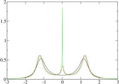
Figure 1: $d$-level spectral function $\rho_{d}(\omega)$ for fixed $U=2$ and inverse temperatures $\beta=4,20,2000$, with the conduction electron bath described in the text

On Fig. 1, we display our results for the impurity-orbital spectral function $\rho_{d}(\omega)$, at three different temperatures (the density of states of the conduction electron bath is chosen as a semi-circle with half-width $\Lambda=6$, the resonant level width is $\Delta_{0}=0.16$ and we take $U=2$). The growth of the Kondo resonance as the temperature is lowered is clearly seen. The temperatures in Fig. 1 have been chosen such as to illustrate three different regimes: for $T\gg T_{K}$, no resonance is seen and the spectral density displays a “pseudogap” separating the two high-energy bands; for $T\simeq T_{K}$ transfer of spectral weight to low energy is seen, resulting in a fully developed Kondo resonance for $T\ll T_{K}$. We have not obtained an analytical determination of the Kondo temperature within the present scheme. In the case of NCA equations, it is possible to derive a set of differential equations in the limit of infinite bandwith which greatly facilitate this. This procedure cannot be applied here, because of the form (27) of the boson propagator. Nevertheless, we checked that the numerical estimates of the width of the Kondo peak is indeed exponentially small in $U$ as in formula (36), see Fig. 2. However, because $U$ is normalized as in (33), (which gives the correct atomic limit), the prefactor inside the exponential appears to be twice too small.

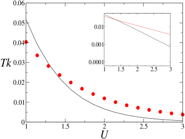
Figure 2: Kondo temperature $T_{K}$ from the exact formula (line) and from the numerical solution of the DSR equations (dots). Units of energy are such that $\Delta_{0}=0.16$.

On Fig. 3, we display the spectral function for a fixed low temperature and increasing values of $U$. The strong reduction of the Kondo scale (resonance width) upon increasing $U$ is clear on this figure. We note that the high-energy peaks have a width which remains of order $\Delta_{0}$, independently of $U$, which is satisfactory. However, we also note that they are not peaked exactly at the atomic value $\pm U/2$, which might be an artefact of these integral equations. The shift is rather small however.

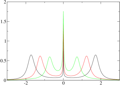
Figure 3: $\rho_{d}(\omega)$ at low temperature ($\beta=600$) and for increasing $U=1,2,3$

Fig. 4 illustrates how the high- and low- energy features in the d-level spectral functions are associated with corresponding features in the auxiliary particle spectral functions $\rho_{f}$ and $\rho_{X}$. In particular, the sigma-model boson (slave rotor) is entirely responsible for the Hubbard bands at high energy (as expected, since it describes charge fluctuations).

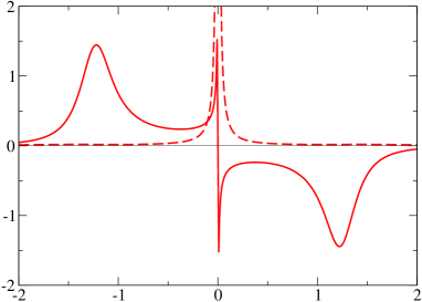
Figure 4: Pseudo-particule spectral function at $U=2$ and $\beta=600$. The Kondo resonance is visible in $\rho_{f}(\omega)$, broken curve, whereas $\rho_{X}(\omega)$ displays higher energy features, plain curve

As stressed in the introduction, an advantage of our scheme is that the d-level self-energy is always causal, even for small $U$ or large doping. This is definitely an improvement as compared to the usual $U$-NCA approximation. This is illustrated by Fig. 5, from which it is also clear that $\Sigma_{d}$ decreases (and eventually vanishes) as $U$ goes to zero (for a more detailed discussion and comparison to NCA, see Sec. III). However, it is also clear from this figure that the low-energy behavior of the self-energy is not consistent with Fermi liquid theory. This is a generic drawback of NCA-like integral equation approaches, that we now discuss in more details.

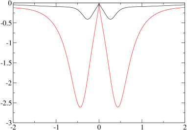
Figure 5: Imaginary part of the physical self-energy on the real-frequency axis, for $U=0.5$ (upper curve) and $U=2$ (lower curve) at $\beta=600$

IV.2 Low-energy behaviour and Friedel sum-rule

We discuss here the low-energy behavior of the integral equations (in the case of a featureless conduction electron bath), for both the d-level and auxiliary field Green’s functions. As explained below, this low-energy behavior depends sensitively on the ratio ${\cal N}=N/M$ which is kept fixed in the limit considered in this paper. The calculations are detailed in Appendix C, where we establish the following.

• Friedel sum rule. The zero-frequency value of the d-level spectral function at $T=0$ is independent of $U$ and reads:

  $$\rho_{d}(\omega=T=0) = \frac{-1}{\pi\Delta^{\prime\prime}(0)}\frac{\pi/2}{{\cal N}+1}\tan\left(\frac{\pi}{2}\frac{{\cal N}}{{\cal N}+1}\right)$$

  (37)

  This is to be contrasted with the exact value for the $O(2)$ model ($M=1$), which is independent of $N$ and reads:

  $$\rho_{d}^{{{\mathrm{exact}}}}(\omega=T=0)=\frac{-1}{\pi\Delta^{\prime\prime}(0)}\;\;\;(M=1,\;\;{{\mathrm{any}}}\;N)$$ (38)

  This is the Friedel sum rule [18, 4], which in this particle-hole symmetric case simply follows from the Fermi-liquid requirement that the (inverse) lifetime $\Sigma^{\prime\prime}_{d}(\omega=0)$ should vanish at $T=0$ (since $G_{d}^{-1}=i\omega-\Delta(i\omega)-\Sigma_{d}(i\omega)$). As a result, $\rho_{d}(0)$ is pinned at its non-interacting value. The integral equations discussed here yield a non-vanishing $\Sigma^{\prime\prime}_{d}(\omega=0)$ (albeit always negative in order to satisfy causality), and hence do not describe a Fermi liquid at low energy. The result (37) is identical to that found in the NCA for $U=\infty$, but holds here for arbitrary $U$. There is actually no contradiction between this remark and the fact that our integral equations yield the exact spectral function in the $U\rightarrow~{}0$ limit. Indeed, the limit $U\rightarrow 0$ at finite $T,\omega$ does not commute with $\omega,T\rightarrow 0$ at finite $U$ (in which (37) holds).

• Low-frequency behavior. The auxiliary particle spectral functions have a low-frequency singularity characterized by exponents which depend continuously on ${\cal N}$ (as in the $U=\infty$ NCA): $\rho_{f}(\omega)\propto 1/\Sigma^{\prime\prime}_{f}(\omega)\propto 1/|\omega|^{\alpha_{f}}$, $\rho_{X}(\omega)\propto 1/\Sigma^{\prime\prime}_{X}(\omega)\propto{{\mathrm{Sign}}}(\omega)/|\omega|^{\alpha_{X}}$, with: $\alpha_{f}=1-\alpha_{X}=1/({\cal N}+1)$. These behavior are characterized more precisely in Appendix C. A power-law behavior is also found for the physical self-energy $\Sigma^{\prime\prime}_{d}(\omega)-\Sigma^{\prime\prime}_{d}(0)$ at low frequency (as evident from Fig. 5).

Let us comment on the origin of these low-energy features, as well as on their consequences for the practical use of the present method.

First, it is clear from expression (21) that the Anderson impurity hamiltonian generalized to ${{\mathrm{SU}}}(N)\times{{\mathrm{O}}}(2M)$ actually involves $M$ channels of conduction electrons. Hence, the non-Fermi liquid behaviour found when solving the integral equations associated with the $N,M\rightarrow\infty$ limit simply follows from the fact that multi-channel models lead to overscreening of the impurity spin, and correspond to a non-Fermi liquid fixed point. In that sense, these integral equations reproduce very accurately the expected low-energy physics, as previously studied for the simplest case of the Kondo model in [11, 12].

Naturally, this means that the use of such integral equations to describe the one-channel (exactly screened) case becomes problematic in the low-energy region. In particular, the exact Friedel sum rule is violated, the d-level lifetime remains finite at low energy and non-Fermi liquid singularities are found. While the approach is reasonable in order to reproduce the overall features of the one-electron spectra, it should not be employed to calculate transport properties at low energy for example. We note however that the deviation from the exact Friedel sum rule vanishes in the ${\cal N}\rightarrow\infty$ limit. This is expected from the fact that in this limit the number of channels ($M$) is small as compared to orbital degeneracy ($N$). The violation of the sum rule remains rather small even for reasonable values of ${\cal N}$. This parameter can actually be used as an adjustable parameter when using the present method as an approximate impurity solver. There is no fundamental reason for which ${\cal N}=N$ should provide the best approximate description of the spectral functions of the one-channel case. We shall use this possibility when applying this method in the DMFT context in the next section: there, we choose ${\cal N}=3$ in order to adjust to the known critical value of $U$ for a single orbital. We also used this value in the calculations reported above. The zero-frequency value of the spectral density is thus $\rho_{d}(0)\simeq 1.85$, while the Friedel sum rule would yield $\rho_{d}(0)\simeq 1.95$ (cf. Fig. 3). Hence the violation of the sum rule is a small effect (of the order of $5\%$), comparable to the one found with ”numerically exact” solvers, due to discretization errors [19]. Also, we point out that the pinning of $\rho_{d}(0)$ at a value independent of $U$ (albeit not that of the Friedel sum-rule) is an important aspect of the present method, which will prove to be crucial in the context of DMFT in order to recover the correct scenario for the Mott transition.

Finally, we emphasize that increasing the parameter ${\cal N}$ also corresponds to increasing the orbital degeneracy of the impurity level. This will be studied in more details in Sec. V.4. In particular, we shall see that correlation effects become weaker as ${\cal N}$ is increased (for a given value of $U$), due to enhanced orbital fluctuations.

V Applications to Dynamical Mean-Field Theory and the Mott transition

V.1 One-orbital case: Mott transition, phase diagram

Dynamical Mean-Field Theory has led to significant progress in our understanding of the physics of a correlated metal close to the Mott transition [2]. The detailed description of this transition itself within DMFT is now well established [2, 7, 20, 22, 21, 19, 15]. In this section, we use these established results as a benchmark and test the applicability of the method introduced in this paper in the context of DMFT, with very encouraging results. As explained above, this is particularly relevant in view of the recent applications of DMFT to electronic structure calculations of correlated solids [5], which call for efficient multi-orbital impurity solvers.

As is well-known [6, 2, 3], DMFT maps a lattice hamiltonian onto a self-consistent quantum impurity model. We discuss first the half-filled Hubbard model, and address later the doped case. We then have to solve a particle-hole symmetric Anderson impurity model :

$$S = \int_{0}^{\beta}\!\!\!\!d\tau\sum_{\sigma}d_{\sigma}^{\dagger}\partial_{\tau}d_{\sigma}+\frac{U}{2}\left[\sum_{\sigma}d_{\sigma}^{\dagger}d_{\sigma}-1\right]^{2}$$

$$+ \int_{0}^{\beta}\!\!\!\!d\tau\int_{0}^{\beta}\!\!\!\!d\tau^{\prime}\;\Delta(\tau-\tau^{\prime})\sum_{\sigma}d_{\sigma}^{\dagger}(\tau)d_{\sigma}(\tau^{\prime})$$

subject to the self-consistency condition:

$$\Delta(\tau)=t^{2}G_{d}(\tau)$$ (40)

In this expression, a semi-circular density of states with half-bandwith $D=2t$ has been considered, corresponding to a infinite-connectivity Bethe lattice ($z=\infty$) with hopping $t_{ij}=t/\sqrt{z}$. In the following, we shall generally express all energies in units of $D$ ($D=1$).

In practice, one must iterate numerically the “DMFT loop”: $\Delta(\tau)\rightarrow G_{d}(\tau)\rightarrow\Delta(\tau)_{new}=t^{2}G_{d}$, using some “impurity solver”. Here, we make use of the integral equations (28-III.2). The hybridization function $\Delta(\tau)$ being determined by the self-consistency condition (40), there are only two free parameters, the local Coulomb repulsion $U$ and the temperature $T$ (normalized by $D$).

We display in Fig. 6 the spectral functions obtained at low temperature, for increasing values of $U$, and in Fig. 7 the corresponding phase diagram. The value of the parameter ${\cal N}$ has been adapted to the description of the one-orbital case (see below). The most important point is that we find a coexistence region at low-enough temperature: for a range of couplings $U_{c1}(T)\leq U\leq U_{c2}(T)$, both a metallic solution and an insulating solution of the (paramagnetic) DMFT equations exist. The Mott transition is thus first-order at finite temperatures. This is in agreement with the results established for this problem by solving the DMFT equations with controlled numerical methods [21, 19], as well as with analytical results [22, 20]. In particular, the spectral functions that we obtain (Fig. 6) display the well-known separation of energy scales found within DMFT: there is a gradual narrowing of the quasiparticle peak, together with a preformed Mott gap at the transition. In the next section, we compare these spectral functions to those obtained using other approximate solvers. As pointed out there, despite some formal similarity in the method, it is well-known that the standard $U$-NCA does not reproduce correctly this separation of energy scales close to the transition [23].

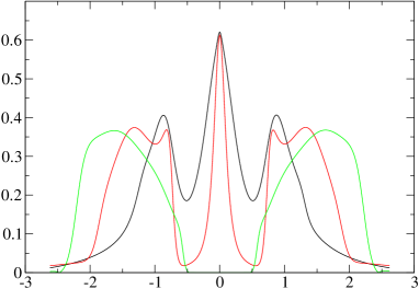
Figure 6: Local spectral function at $\beta=40$ and $U=1,2,3$ for the half-filled Hubbard model within DMFT, as obtained with the DSR solver

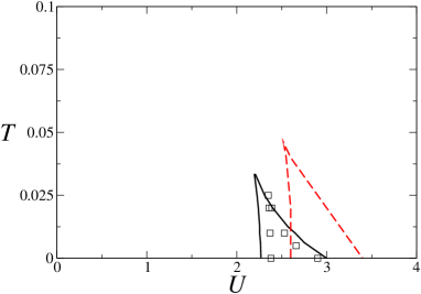
Figure 7: Single-orbital (paramagnetic) phase diagram at half-filling. Squares indicate the ED result, the DSR result is the solid line, and IPT the broken line

Let us explain how the parameter ${\cal N}$ has been chosen in these calculations. As demonstrated below, the values of the critical couplings $U_{c1}$ and $U_{c2}$ (and hence the whole phase diagram and coexistence window) strongly depends on the value of this parameter. This is expected, since ${\cal N}$ is a measure of orbital degeneracy. What has been done in the calculations displayed above is to choose ${\cal N}$ in such a way that the known value [20] $U_{c2}(T=0)\simeq 2.9$ of the critical coupling at which the $T=0$ metallic solution disappears in the single-orbital case, is accurately reproduced. We found that this requires ${\cal N}\simeq 3$ (note that $N/M=2$ in the one-orbital case, so that the best agreement is not found by a naive application of the large $N,M$ limit). This value being fixed, we find a critical coupling $U_{c1}(T=0)\simeq 2.3$ in good agreement with the value from (adaptative) exact diagonalizations $U_{c1}\simeq 2.4$. The whole domain of coexistence in the $(U,T)$ plane is also in good agreement with established results (in particular we find the critical endpoint at $T_{c}\simeq 1/30$, while QMC yields $T_{c}\simeq 1/40$). These are very stringent tests of the applicability of the present method, since we have allowed ourselves to use only one adjustable parameter (${\cal N}$). In Sec.V.4, we study how the Mott transition depends on the number of orbitals, which further validates the procedure followed here.

V.2 Comparison to other impurity solvers: spectral functions

Let us now compare the spectral functions obtained by the present method with other impurity solvers commonly used for solving the DMFT equations. We start with the iterated perturbation theory approximation (IPT) and the exact diagonalization method (ED). Both methods have played a major role in the early developments of the DMFT approach to the Mott transition [7]. A comparison of the spectral functions obtained by the present method to those obtained with IPT and ED is displayed in Fig. 8, for a value of $U$ corresponding to a correlated metal close to the transition.

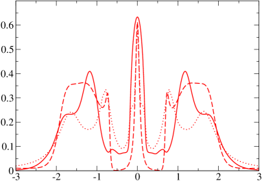
Figure 8: Comparison between DSR (dash), IPT (straight) and ED (dot) at $U=2.4$ and $\beta=60$

The overall shape and characteristic features of the spectral function are quite similar for the three methods. A narrow quasiparticle peak is formed, together with Hubbard bands, and there is a clear separation of energy scales between the width of the central peak (related to the quasiparticle weight) and the “preformed” Mott (pseudo-)gap associated with the Hubbard bands: this is a distinguishing aspect of DMFT. It is crucial for an approximate solver to reproduce this separation of energy scales in order to yield a correct description of the Mott transition and phase diagram.

There are of course some differences between the three methods, on which we now comment. First, we note that the IPT approximation has a somewhat larger quasiparticle bandwith. This is because the transition point $U_{c2}$ is overestimated within IPT (cf. Fig. 7), so that a more fair comparison should perhaps be made at fixed $U/U_{c2}$. It is true however, that the DSR method has a tendency to underestimate the quasiparticle bandwith, and particularly at smaller values of $U$. Accordingly, the Hubbard bands have a somewhat too large spectral weight, but are correctly located in first approximation. The detailed shape of the Hubbard bands is not very accurately known, in any case. (The ED method involves a broadening of the delta-function peaks obtained by diagonalizing the impurity hamiltonian with a limited number of effective orbitals, so that the high-energy behaviour is not very accurate on the real axis. This is also true, actually, of the more sophisticated numerical renormalization group). We emphasize that, since the DSR method does not have the correct low-frequency Fermi liquid behaviour, the quasiparticle bandwith should be interpreted as the width of the central peak in $\rho_{d}(\omega)$ (while the quasiparticle weight $Z$ cannot be defined formally).

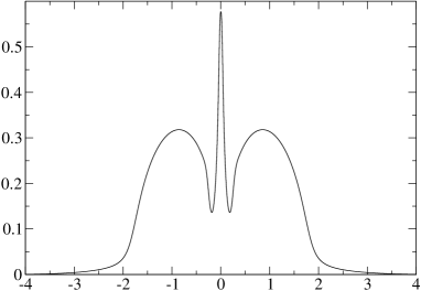
Figure 9: $U$-NCA spectral function for $U=1.5$ at low temperature.

In Fig 9 and Fig. 10, we display the spectral functions obtained by using the NCA method (extended at finite $U$ in the simplest manner). It is clear that the $U$-NCA underestimates considerably the quasiparticle bandwith (and thus yields a Mott transition at a rather low value of the coupling). This is not very surprising, since this method is based on a strong coupling expansion around the atomic limit, and one could think again of a comparison for fixed $U/U_{c}$. More importantly, the $U$-NCA misses the important separation of energy scales between the central peak and the Mott gap. As a result, it does not reproduce correctly the phase diagram for the Mott transition within DMFT (in particular regarding coexistence). A related key observation is that the $U$-NCA does not have the correct weak-coupling (small $U$) limit. To illustrate this point, we display in Fig. 10 the $U$-NCA and DSR spectral functions for a tiny value of the interaction $U/D=0.1$: the DSR result is shown to approach correctly the semi-circular shape of the non-interacting density of states, while the $U$-NCA displays a characteristic inverted V-shape: in this regime the violation of the Friedel sum rule becomes large and the negative lifetime pathology is encountered within $U$-NCA. In contrast, the DSR yields a pinning of the spectral density at a $U$-independent value and does not lead to a violation of causality. It should be emphasized however that, even though it yields the exact $U=0$ density of states at $T=0$, the DSR method is not quantitatively very accurate in the weak-coupling regime.

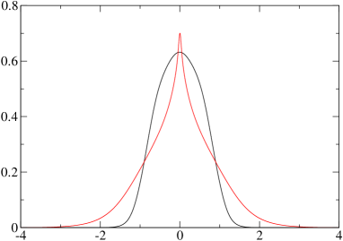
Figure 10: Results for $U=0.1$ showing how $U$-NCA overshoots the Friedel’s sum rule. The Slave Rotor method is correctly converging towards the free density of states (semi-circular)

V.3 Double occupancy

Finally, we demonstrate that two-particle correlators in the charge sector can also be reliably studied with the DSR method, taking the fraction of doubly occupied sites $d_{\uparrow\downarrow}\equiv\left<n_{\uparrow}n_{\downarrow}\right>$ as an example.

Using the constraint (4), we calculate the connected charge susceptibility in the following manner:

$$\chi_{c}(\tau) \equiv \left<\sum_{\sigma}\left(n_{\sigma}(\tau)-\frac{1}{2}\right)\sum_{\sigma^{\prime}}\left(n_{\sigma^{\prime}}(0)-\frac{1}{2}\right)\right>$$

$$= \left<\hat{L}(\tau)\hat{L}(0)\right>=\frac{1}{U^{2}}\left<\partial_{\tau}\theta(\tau)\partial_{\tau}\theta(0)\right>$$

$$= \frac{2}{U^{2}}\left[G_{X}(\tau)\partial_{\tau}^{2}G_{X}(\tau)+U\delta(\tau)-(\partial_{\tau}G_{X}(\tau))^{2}\right]$$

The double occupancy is obtained by taking the equal-time value:

$$\chi_{c}(\tau=0)=2\left<n_{\uparrow}n_{\downarrow}\right>=2d_{\uparrow\downarrow}$$ (42)

In Fig. 11, we plot the double occupancy obtained in that manner, in comparison to the ED and IPT results. Within ED, $d_{\uparrow\downarrow}$ is calculated directly from the charge correlator. Within IPT, $\chi_{c}(\tau)$ is not approximated very reliably [24], but the double occupancy can be accurately calculated by taking a derivative of the internal energy with respect to $U$.

Fig. 11 demonstrates that the DSR method is very accurate in the Mott transition region and in the insulator. In particular, the hysteretic behaviour is well reproduced. In the weak coupling regime however, the approximation deteriorates. This issue actually depends on the quantity: the physical Green’s function has the correct limit $U\rightarrow 0$, as emphasized above, but this is not true for the charge susceptibility (hence for $d_{\uparrow\downarrow}$). The mathematical reason is that the constraint (4) is crucial for writing (V.3), but this constraint is only treated on average within our method. This shows the inherent limitations of slave-boson techniques for evaluating two-particle properties. The frequency dependence of two-particle correlators will be dealt with in a forthcoming publication.

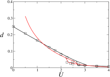
Figure 11: Double occupancy at $\beta=80$ as a function of $U$. The ED result is indicated with squares. DSR overshoots the exact result on the left, whereas IPT is slightly displaced to the right.

V.4 Multi-orbital effects

In this section, we apply the DSR method to study the dependence of the Mott transition on orbital degeneracy $N$. We emphasize that there are at this stage very few numerical methods which can reliably handle the multi-orbital case, specially when $N$ becomes large. Multi-orbital extensions of IPT have been studied [8], but the results are much less satisfactory than in the one-orbital case. The ED method is severely limited by the exponential growth of the size of the Hilbert space. The Mott transition has been studied in the multi-orbital case using QMC, with a recent study [25] going up to $N=8$ (4 orbitals with spin). Furthermore, we have recently obtained [15] some analytical results on the values of the critical couplings in the limit of large-$N$. Those, together with the QMC results, can be used as a benchmark of the DSR approximation presented here. As explained above, a value of ${\cal N}_{N=2}\simeq 3$ was found to describe best the single orbital case ($N=2$). Hence, upon increasing $N$, we choose the parameter ${\cal N}$ such that ${\cal N}_{N}/{\cal N}_{N=2}=N/2$.

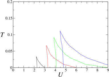
Figure 12: Instability lines $U_{c1}(T)$,$U_{c2}(T)$, and coexistence region for one, two, three and four orbitals ($N=2,4,6,8$) as obtained by DMFT (DSR solver)

In Fig. 12, we display the coexistence region in the $(U,T)$ plane for increasing values of $N$, as obtained with DSR. The values of the critical interactions grow with $N$. A fit of the transition lines $U_{c1}(T)$ (where the insulator disappears) and $U_{c2}(T)$ (where the metal disappears) yields:

$$U_{c1}(N,T) = A_{1}(T)\sqrt{N}$$ (43)

$$U_{c2}(N,T) = A_{2}(T)N$$ (44)

These results are in good accordance with both the QMC data [25], and the exact results established in [15]. When increasing the number of orbitals, the coexistence region widens and the critical temperature associated with the endpoint of the Mott transition line also increases.

We display on Fig. 13 the DSR result for the spectral function for $N=2$ and $N=4$, at a fixed value of $U$ and $T$. Two main effects should be noted. First, correlations effects in the metal become weaker as $N$ is increased (for a fixed $U$), as clear e.g from the increase of the quasiparticle bandwith. This is due to increasing orbital fluctuations. Second, the Hubbard bands also shift towards larger energies, an effect which can be understood in the way atomic states broadens in the insulator [26].

To conclude this section, we have found that the DSR yields quite satisfactory results when used in the DMFT context for multi-orbital models. In the future, we plan to use this method in the context of realistic electronic structure calculations combined with DMFT, in situations where “numerically exact” solvers (e.g QMC) become prohibitively heavy. There are however some limitations to the use of DSR (at least in the present version of the approach), which are encountered when the occupancy is not close to $N/2$. We examine this issue in the next section.

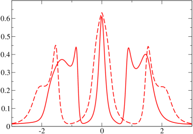
Figure 13: Spectral function at $U=2$, $\beta=60$ and for one (full line) and two orbitals (broken line)

V.5 Effects of doping

Up to now, we studied the half-filled problem (i.e. containing exactly $N/2$ electrons), with exact particle-hole symmetry. In that case, $\epsilon_{0}\equiv\epsilon_{d}+U/2=0$ and the Lagrange multiplier $h$ enforcing the constraint (III.2) could be set to $h=0$. In realistic cases, particle-hole symmetry will be broken (so that $\epsilon_{0}\neq 0$), and we need to consider fillings different from $N/2$. Hence, the Lagrange multiplier $h$ must be determined in order to fulfill (III.2), which we rewrite more explicitly as:

$$n_{f} = \frac{1}{2}-\frac{2h}{{\cal N}U}$$

$$+ \frac{1}{{\cal N}U}\frac{1}{\beta}\sum_{n}\frac{-i\nu_{n}\left(e^{i\nu_{n}0^{+}}+e^{i\nu_{n}0^{-}}\right)}{\nu_{n}^{2}/U+\lambda-2ih\nu_{n}/U-\Sigma_{X}(i\nu_{n})}$$

In this expression, $n_{f}=\frac{1}{N}\sum_{\sigma}\langle f^{\dagger}_{\sigma}f_{\sigma}\rangle=\frac{1}{N}\sum_{\sigma}\langle d^{\dagger}_{\sigma}d_{\sigma}\rangle$ is the average occupancy per orbital flavor. (Note that the number of auxiliary fermions and physical fermions coincide, as clear from (34)). $n_{f}$ is related to the d-level position (or chemical potential, in the DMFT context) by:

$$n_{f}=\frac{1}{\beta}\sum_{n}\frac{e^{i\omega_{n}0^{+}}}{i\omega_{n}-\epsilon_{0}+h-\Sigma_{f}(i\omega_{n})}$$ (46)

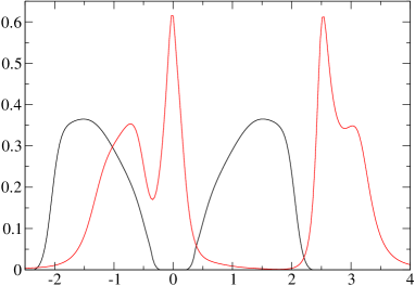
Figure 14: Doping the insulator ($U=3$ and $\beta=60$) with $\epsilon_{0}=0,1$ (corresponding to $n_{f}=0.5,0.4$ respectively)

We display in Fig. 14 the spectral function obtained with the DSR solver when doping the Mott insulator away from half-filling. A critical value of the chemical potential (i.e. of $\epsilon_{0}$) is required to enter the metallic state. The spectral function displays the three expected features: a lower and upper Hubbard bands, as well as a quasiparticle peak (which in this case where the doping is rather large, is located almost at the top of the lower Hubbard band). However, it is immediately apparent from this figure that the DSR method in the doped case overestimates the spectral weight of the upper Hubbard band. This can be confirmed by a comparison to other solvers (e.g ED). Note that the energy scale below which a causality violation appears within U-NCA becomes rapidly large as the system is doped, while no such violation occurs within DSR.

The DSR method encouters severe limitations however as the total occupancy becomes very different from $N/2$. This is best understood by studying the dependence of the occupancy upon $\epsilon_{0}$, in the atomic limit. As explained in Appendix. A, the use of sigma-model variables $X$ (in the large-$M$ limit) results in a poor description of the $n_{f}$ vs. $\epsilon_{0}$ dependence (“Coulomb staircase”). As a result, it is not possible to describe the Mott transitions occurring in the multi-orbital model at integer fillings different from $N/2$ using the DSR approximation. It should be emphasized however that this pathology is only due to the approximation of the $O(2)$ quantum rotor $e^{i\theta}$ by a $O(M)$ sigma-model field. A perfect description of the Coulomb staircase is found for all fillings when treating the constraint (4) on average while keeping a true quantum rotor [27]. Hence, it seems feasible to overcome this problem and extend the practical use of the (dynamical) slave rotor approach to all fillings. We intend to address this issue in a future work.

VI Conclusion

We conclude by summarizing the strong points as well as the limitations of the new quantum impurity solver introduced in this paper, as well as possible extensions and applications.

On the positive side, the DSR method provides an interpolating scheme between the weak coupling and atomic limits (at half-filling). It is also free of some of the pathologies encountered in the simplest finite-$U$ extensions of NCA (negative lifetimes at low temperature). When applied in the context of DMFT, it is able to reproduce many of the qualitatively important features associated with the Mott transition, such as coexisting insulating and metallic solutions and the existence of two energy scales in the DMFT description of a correlated metal (the quasi-particle coherence bandwith and the “preformed gap”). Hence the DSR solver is quite useful in the DMFT context, at a low computational cost, and might be applicable to electronic structure calculations for systems close to half-filling when the orbital degeneracy becomes large. To incorporate more realistic modelling, one can introduce different energy levels for each correlated orbital, while the extension to non-symmetric Coulomb interactions (such as the Hund’s coupling) may require some additional work.

The DSR method does not reproduce Fermi-liquid behaviour at low energy however, which makes it inadequate to address physical properties in the very low-energy regime (as is also the case with NCA). The main limitation however is encountered when departing from half-filling (i.e from $N/2$ electrons in an $N$-fold degenerate orbital). While the DSR approximation can be used at small dopings, it fails to reproduce the correct atomic limit when the occupancy differs significantly from $N/2$ (and in particular cannot deal with the Mott transition at other integer fillings in the multi-orbital case). We would like to emphasize however that this results from extending the slave rotor variable to a field with a large number of components. It is possible to improve this feature of the DSR method by dealing directly with an $O(2)$ phase variable, which does reproduce accurately the atomic limit even when the constraint is treated at the mean-field level. We intend to address this issue in a future work. Another possible direction is to examine systematic corrections beyond the saddle-point approximation in the large $N,M$ expansion.

Finally, we would like to outline some other possible applications of the slave rotor representation introduced in this paper (Sec. II). This representation is both physically natural and economical. In systems with strong Coulomb interactions, the phase variable dual to the local charge is an important collective field. Promoting this single field to the status of a slave particle avoids the redundancies of usual slave-boson representations. In forthcoming publications, we intend to use this representation for: i) constructing impurity solvers in the context of extended DMFT [29], in which the frequency-dependent charge correlation function must be calculated [28] ii) constructing mean-field theories of lattice models of correlated electrons (e.g the Hubbard model) [27] and iii) dealing with quantum effects on the Coulomb blockade in mesoscopic systems.

Appendix A The Atomic limit

In this appendix we prove the claim that the atomic limit of the model is exact at half-filling and at zero temperature (at finite temperature, deviations from the exact result are of order $\exp{(-\beta U)}$ and therefore negligeable for pratical purposes). To do this, we first extract the values of the mean-field parameters $\lambda$ and $h$ from the saddle-point equations at zero temperature and $\Delta(\tau)\equiv 0$.

$$1 = \int\!\frac{{{\mathrm{d}}}\nu}{2\pi}\frac{1}{\frac{\nu^{2}}{U}+\lambda+\frac{2ih\nu}{U}}$$ (47)

$$\theta(h-\epsilon_{0}) = \frac{1}{2}-\frac{2h}{{\cal N}U}+\frac{4h}{{\cal N}U^{2}}\int\!\frac{{{\mathrm{d}}}\nu}{2\pi}\frac{\nu^{2}}{\left(\frac{\nu^{2}}{U}+\lambda\right)^{2}+\left(\frac{2h\nu}{U}\right)^{2}}$$

Performing the integrals shows that $\lambda=(U^{2}-4h^{2})/(4U)$ and $\theta(h-\epsilon_{0})=1/2$, so that $h=\epsilon_{0}$. If $|\epsilon_{0}|>U/2$, the equations lead actually to a solution with an empty or full valence that we show on Fig. 15.

We can now compute the physical Green’s function $G_{d}(\tau)=G_{f}(\tau)G_{X}(-\tau)$ from the pseudo-propagators $G_{f}(i\omega_{n})=1/(i\omega_{n})$ and:

$$G_{X}(i\nu_{n}) = \frac{1}{\nu_{n}^{2}/U+(U/4-\epsilon_{0}^{2}/U)-2i\epsilon_{0}\nu_{n}/U}$$

$$= \frac{-1}{i\nu_{n}+\epsilon_{0}-U/2}+\frac{1}{i\nu_{n}+\epsilon_{0}+U/2}$$

Performing the convolution in imaginary frequency and taking the limit $T=0$ leads to:

$$G_{d}(i\omega_{n}) = \frac{1}{\beta}\sum_{i\nu_{n}}G_{X}(i\nu_{n})G_{f}(i\omega_{n}+i\nu_{n})$$ (49)

$$= \frac{1/2}{i\omega_{n}-\epsilon_{0}+U/2}+\frac{1/2}{i\omega_{n}-\epsilon_{0}-U/2}$$ (50)

Because $\epsilon_{0}=-\mu+U/2$ this is the correct atomic limit of the single-band model (at half-filling). The result for the empty or full orbital is however not accurate, as shown in figure 15. This discrepancy with the correct result (even for one orbital) finds its root in the large $M$ treatment of the slave rotor $X$.

Figure 15: Impurity occupancy in function of the $d$-level position in the rotor description (full curve) and the exact result (dot curve), in the two-orbital case.

Appendix B Numerical solution of the real time equations

Here we show how the saddle-point equations (28-III.2) can be analytically continued along the real axis. We start with $\Sigma_{X}(\tau)=-{\cal N}\Delta(\tau)G_{f}(-\tau)$, which can be first Fourier transformed into:

$$\Sigma_{X}(i\nu_{n})= \!\!\!\!\!\int_{0}^{\beta}\!\!\!\!d\tau\;\Sigma_{X}(\tau)e^{i\nu_{n}\tau}$$ (51)

$$=-{\cal N}\int\frac{{{\mathrm{d}}}\epsilon_{1}}{\pi} \!\!\!\!\!\!G_{f}^{\prime\prime}(\epsilon_{1})\int\frac{{{\mathrm{d}}}\epsilon_{2}}{\pi}\Delta^{\prime\prime}(\epsilon_{2})\frac{n_{F}(\epsilon_{1})-n_{F}(\epsilon_{2})}{i\nu_{n}+\epsilon_{1}-\epsilon_{2}}$$

where we used the spectral representation

$$G(z)=-\int\frac{{{\mathrm{d}}}\omega}{\pi}\frac{G^{\prime\prime}(\epsilon)}{z-\epsilon}$$ (52)

for each Green’s function. The notations here are quite standard: $G^{\prime\prime}(\epsilon)\equiv{\mathcal{I}}m\,G(\epsilon+i0^{+})$, $n_{F}(\epsilon)$ is the Fermi factor, and $n_{B}(\epsilon)$ denotes the Bose factor.

It is then immediate to continue $i\nu_{n}\rightarrow\nu+i0^{+}$ in equation (51), and using again the spectral decomposition (52), we derive an equation between retarded quantities:

$$\Sigma_{X}(\nu) = -{\cal N}\int\frac{{{\mathrm{d}}}\epsilon}{\pi}G_{f}^{\prime\prime}(\epsilon)n_{F}(\epsilon)\Delta(\epsilon+\nu)$$

$$-{\cal N}\int\frac{{{\mathrm{d}}}\epsilon}{\pi}\Delta^{\prime\prime}(\epsilon)n_{F}(\epsilon)G_{f}(\epsilon-\nu)$$

A calculation along the same lines for the fermionic self-energy $\Sigma_{f}(\tau)=\Delta(\tau)G_{X}(\tau)$ leads to:

$$\Sigma_{f}(\omega) = -\int\frac{{{\mathrm{d}}}\epsilon}{\pi}G_{X}^{\prime\prime}(\epsilon)n_{B}(\epsilon)\Delta(\omega-\epsilon)$$

$$-\int\frac{{{\mathrm{d}}}\epsilon}{\pi}\Delta^{\prime\prime}(\epsilon)n_{F}(\epsilon)G_{X}(\omega-\epsilon)$$

The numerical implementation is then straightforward because (B) and (B) can each be expressed as the convolution product of two quantities, so that they can be calculated rapidly using FFT. The algorithm is looped back using the Dyson equations (for real frequency):

$$G^{-1}_{f}(\omega) = \omega-\epsilon_{0}+h-\Sigma_{f}(\omega)$$ (55)

$$G^{-1}_{X}(\nu) = -\frac{\nu^{2}}{U}+\lambda+\frac{2h\nu}{U}-\Sigma_{X}(\nu)$$ (56)

At each iteration, $\lambda$ and $h$ are determined using a bisection on the equations (30-III.2), which can be properly expressed in terms of retarded Green’s functions:

$$1 = \int\frac{{{\mathrm{d}}}\epsilon}{\pi}G_{X}^{\prime\prime}(\epsilon)n_{B}(\epsilon)$$ (57)

$$n_{f} = \frac{1}{2}-\frac{2h}{{\cal N}U}-\frac{2}{{\cal N}U}\int\frac{{{\mathrm{d}}}\epsilon}{\pi}G_{X}^{\prime\prime}(\epsilon)\epsilon n_{B}(\epsilon)$$ (58)

where $n_{f}$, the average number of physical fermions, is:

$$n_{f}=G_{f}(\tau\!=\!0^{-})=-\int\frac{{{\mathrm{d}}}\epsilon}{\pi}G_{f}^{\prime\prime}(\epsilon)n_{F}(\epsilon)$$ (59)

We note here that solving these real-time integral equations can be quite difficult deep in the Kondo regime of the Anderson model, or very close to the Mott transition for the full DMFT equations. The reason is that $G_{f}(\omega)$ and $G_{X}(\omega)$ develop low energy singularities (this is analytically shown in the next appendix), that make the numerical resolution very unprecise if one uses FFT. In that case, it is necessary to introduce a logarithmic mesh of frequency (loosing the benefit of the FFT speed, but increasing the accuracy), or to perform a Padé extrapolation of the imaginary time solution.

Appendix C Friedel’s sum rule

We present here for completeness the derivation of the Slave Rotor Friedel’s sum rule, equation (37), at half-filling. The idea, motivated by the numerical analysis as well as theoretical arguments [30, 12], is that the pseudo-particles develop low frequency singularities at zero temperature:

$$G_{f}^{\prime\prime}(\omega) = A_{f}|\omega|^{-\alpha_{f}}$$ (60)

$$G_{X}^{\prime\prime}(\omega) = A_{X}|\omega|^{-\alpha_{X}}{{\mathrm{Sign}}}(\omega)$$ (61)

Using the spectral representation

$$G(\tau)=\int_{0}^{+\infty}\frac{{{\mathrm{d}}}\omega}{\pi}\;e^{-\omega\tau}G^{\prime\prime}(\omega)$$ (62)

we deduce the long time behavior of the Green’s functions (we denote by $\Gamma(z)$ the gamma function):

$$G_{f}(\tau) = \frac{A_{f}\Gamma(1-\alpha_{f})}{\pi}\frac{{{\mathrm{Sign}}}(\tau)}{|\tau|^{1-\alpha_{f}}}$$ (63)

$$G_{X}(\tau) = \frac{A_{X}\Gamma(1-\alpha_{X})}{\pi}\frac{1}{|\tau|^{1-\alpha_{X}}}$$ (64)

We have similarly

$$\Delta(\tau)=\frac{\Delta^{\prime\prime}(0)}{\pi\tau}$$ (65)

if one assumes a regular bath density of states at zero frequency. The previous expressions allow to extract the long time behavior of the pseudo-self-energies (using the saddle-point equations (28-29)):

$$\Sigma_{X}(\tau) = \frac{{\cal N}A_{f}\Gamma(1-\alpha_{f})}{\pi^{2}}\frac{\Delta^{\prime\prime}(0)}{|\tau|^{2-\alpha_{f}}}$$ (66)

$$\Sigma_{f}(\tau) = \frac{A_{X}\Gamma(1-\alpha_{X})}{\pi^{2}}\frac{\Delta^{\prime\prime}(0)\;{{\mathrm{Sign}}}(\tau)}{|\tau|^{2-\alpha_{X}}}$$ (67)

The next step is to use (62) the other way around to get from (66-67) the $\omega$-dependance of the self-energies:

$$\Sigma_{X}^{\prime\prime}(\omega) = \frac{{\cal N}}{\pi}\frac{A_{f}\Delta^{\prime\prime}(0)}{1-\alpha_{f}}|\omega|^{1-\alpha_{f}}\;{{\mathrm{Sign}}}(\omega)$$ (68)

$$\Sigma_{f}^{\prime\prime}(\omega) = \frac{1}{\pi}\frac{A_{X}\Delta^{\prime\prime}(0)}{1-\alpha_{X}}|\omega|^{1-\alpha_{X}}$$ (69)

It is necessary at this point to calculate the real part of both self-energies. This can be done using the Kramers-Kronig relation, but analyticity provides a simpler route. Indeed, by noticing that $\Sigma(z)$ is an analytic function of $z$ and must be uni-valuated above the real axis , we find:

$$\Sigma_{X}(z) = \frac{{\cal N}}{\pi}\frac{A_{f}\Delta^{\prime\prime}(0)}{1-\alpha_{f}}\frac{e^{i(\alpha_{f}-1)\pi/2}}{\sin[(\alpha_{f}-1)\pi/2]}|z|^{1-\alpha_{f}}$$

$$\Sigma_{f}(z) = \frac{1}{\pi}\frac{A_{X}\Delta^{\prime\prime}(0)}{1-\alpha_{X}}\frac{e^{i\alpha_{X}\pi/2}}{\sin[\alpha_{X}\pi/2]}|z|^{1-\alpha_{X}}$$

The same argument shows from (60-61) that:

$$G_{f}(z) = A_{f}\frac{e^{i(\alpha_{f}+1)\pi/2}}{\sin[(\alpha_{f}+1)\pi/2]}|z|^{-\alpha_{f}}$$ (70)

$$G_{X}(z) = A_{X}\frac{e^{i\alpha_{X}\pi/2}}{\sin[\alpha_{X}\pi/2]}|z|^{-\alpha_{X}}$$ (71)

We can therefore collect the previous expressions, using Dyson’s formula for complex argument:

$$G^{-1}_{f}(z) = z-\Sigma_{f}(z)$$ (72)

$$G^{-1}_{X}(z) = -\frac{z^{2}}{U}+\lambda-\Sigma_{X}(z)$$ (73)

and this enables us to extract the leading exponents, as well as the product of the amplitudes:

$$\alpha_{f} = \frac{1}{{\cal N}+1}$$ (74)

$$\alpha_{X} = \frac{{\cal N}}{{\cal N}+1}$$ (75)

$$A_{f}A_{X} = \frac{\pi}{{\cal N}+1}\frac{1}{\Delta^{\prime\prime}(0)}\sin^{2}\left(\frac{\pi}{2}\frac{{\cal N}}{{\cal N}+1}\right)$$ (76)

We finish by computing the long time behavior of the physical Green’s function $G_{d}(\tau)=G_{f}(\tau)G_{X}(-\tau)$ together with equations (63-64):

$$G_{d}(\tau)=\frac{\pi}{2({\cal N}+1)}\tan\left(\frac{\pi}{2}\frac{{\cal N}}{{\cal N}+1}\right)\frac{1}{\pi\Delta^{\prime\prime}(0)}\frac{1}{\tau}$$ (77)

This proves (37). In principle, next leading order corrections can be computed by the same line of arguments, although this is much more involved [12]. Non Fermi Liquid correlations in the physical Green’s function would appear in this computation.

References

- [1] For an introduction, see: L. Kouwenhoven and L. Glazman, Phys. World 14, 33 (2001)
- [2] For a review, see: A. Georges, G. Kotliar, W. Krauth and M. Rozenberg, Rev. Mod. Phys. 68, 13 (1996)
- [3] For a review, see: T. Pruschke, M. Jarrell, and J.K. Freericks, Adv. Phys. 42, 187 (1995)
- [4] See e.g: A. Hewson, ”The Kondo problem to heavy fermions” (Cambridge)
-
[5]
For recent reviews, see: ”Strong Coulomb Correlations in Electronic Structure Calculations”
(Advances in Condensed Matter Science),
Edited by V. Anisimov. Taylor and Francis (2001)
K.Held et al. in “Quantum Simulations of Complex Many-Body Systems” Edited by: J. Grotendorst, D. Marx and A. Muramatsu (NIC - Serie Band 11) cond-mat/0112079. - [6] A. Georges and G. Kotliar, Phys. Rev. B 45, 6479 (1992)
- [7] X.Y. Zhang, M. J. Rozenberg, and G. Kotliar, Phys. Rev. Lett. 70, 1666, (1993); A. Georges and W. Krauth, Phys. Rev. B 48, 7167 (1993); M.J. Rozenberg, G. Kotliar and X.Y. Zhang, Phys. Rev. B 49, 10181 (1994).
-
[8]
G. Kotliar and H. Kajueter, Phys. Rev. B 54, R14221 (1996)
H. Kajueter and G. Kotliar, Int. J. Mod. Phys. 11, 729 (1997) - [9] N. Bikers, Rev. Mod. Phys. 59, 845 (1993)
- [10] T. Pruschke and N. Grewe, Z. Phys. B 74, 439 (1989)
- [11] D.L. Cox and A.E. Ruckenstein, Phys. Rev. Lett. 71, 1613 (1993)
-
[12]
O. Parcollet, A. Georges, G. Kotliar and A. Sengupta,
Phys. Rev. B 58, 3794 (1998)
O. Parcollet, PhD thesis, unpublished. - [13] J. Kroha and P. Wölfle, cond-mat/0105491
- [14] G. Kotliar and A.E. Ruckenstein, Phys. Rev. Lett. 57, 1362 (1986)
- [15] S. Florens, A. Georges, G. Kotliar and O. Parcollet, cond-mat/0205263
- [16] T. Pruschke, private communication
- [17] S. Pairault, D. Senechal and A-M. Tremblay, Eur. Phys. J. B 16, 85 (2000)
- [18] K. Yamada, Prog. Theo. Phys. 53, 970 (1975)
- [19] R. Bulla, A.C. Hewson and T. Pruschke, J. Phys: Condens Matter 10 8365 (1998); R. Bulla, T.A. Costi and D. Vollhardt Phys. Rev. B 64, 045103 (2001)
- [20] G. Moeller, Q. Si, G. Kotliar, M. Rozenberg and D.S. Fisher, Phys. Rev. Lett. 74, 2082 (1995)
- [21] M.J. Rozenberg, R. Chitra and G. Kotliar, Phys. Rev. Lett 83, 3498 (1999). W. Krauth, Phys. Rev. B 62, 6860 (2000); J. Joo and V. Oudovenko Phys. Rev. B 64, 193102 (2001)
- [22] G. Kotliar, Eur. Phys. J. B, 11, 27 (1999); G. Kotliar, E. Lange and M.J. Rozenberg, Phys. Rev. Lett. 84, 5180 (2000).
-
[23]
T. Pruschke, D.L. Cox and M. Jarrell, Phys. Rev. B 47, 3553 (1993)
P. Lombardo and G. Albinet, Phys. Rev. B 65, 115110 (2002) - [24] J.K Freericks and M. Jarrell, Phys. Rev. B 50, 6939 (1994)
- [25] B. Amadon and S. Biermann, unpublished
- [26] J.E. Han, M. Jarrell and D.L. Cox, Phys. Rev. B 58, R4199 (1998)
- [27] S. Florens and A. Georges, in preparation
- [28] S. Florens, L. de Medici and A. Georges in preparation
- [29] Q. Si and J. L. Smith, Phys. Rev. Lett. 77, 3391 (1996); H. Kajueter PhD thesis Rutgers University, 1996; J.L. Smith and Q. Si, Phys. Rev. B 61, 5184 (2000); A.M. Sengupta and A. Georges Phys. Rev. B 52 10295 (1995).
- [30] E. Mueller-Hartmann, Z. Phys. B 57,281 (1984)