Generalized two-leg Hubbard ladder at half-filling:
Phase diagram and quantum criticalities

Abstract

The ground-state phase diagram of the half-filled two-leg Hubbard ladder with inter-site Coulomb repulsions and exchange coupling is studied by using the strong-coupling perturbation theory and the weak-coupling bosonization method. Considered here as possible ground states of the ladder model are four types of density-wave states with different angular momentum ($s$-density-wave state, $p$-density-wave state, $d$-density-wave state, and $f$-density-wave state) and four types of quantum disordered states, i.e., Mott insulating states (S-Mott, D-Mott, S’-Mott, and D’-Mott states, where S and D stand for $s$- and $d$-wave symmetry). The $s$-density-wave state, the $d$-density-wave state, and the D-Mott state are also known as the charge-density-wave state, the staggered-flux state, and the rung-singlet state, respectively. Strong-coupling approach naturally leads to the Ising model in a transverse field as an effective theory for the quantum phase transitions between the staggered-flux state and the D-Mott state and between the charge-density-wave state and the S-Mott state, where the Ising ordered states correspond to doubly degenerate ground states in the staggered-flux or the charge-density-wave state. From the weak-coupling bosonization approach it is shown that there are three cases in the quantum phase transitions between a density-wave state and a Mott state: the Ising (Z₂) criticality, the SU(2)₂ criticality, and a first-order transition. The quantum phase transitions between Mott states and between density-wave states are found to be the U(1) Gaussian criticality. The ground-state phase diagram is determined by integrating perturbative renormalization-group equations. It is shown that the S-Mott state and the staggered-flux state exist in the region sandwiched by the charge-density-wave phase and the D-Mott phase. The $p$-density-wave state, the S’-Mott state, and the D’-Mott state also appear in the phase diagram when the next-nearest-neighbor repulsion is included. The correspondence between Mott states in extended Hubbard ladders and spin liquid states in spin ladders is also discussed.

I Introduction

Ladder systems have been studied intensively over the years as a simplified model system that shows variety of quantum phenomena due to strong electron correlations.Dagotto Since the ladder models can be analyzed with powerful nonperturbative methods such as bosonization and conformal field theory as well as with large-scale numerical calculations, they provide a useful testing ground of various theoretical ideas developed for the two-dimensional case. Moreover, the studies of ladder systems have been strongly stimulated by experimental developments in synthesizing compounds with ladder structure that show superconductivity and spin-liquid behavior.Azuma ; Ishida ; Kojima A good example is the ladder compound Sr₁₄Cu₂₄O₄₁ that shows $d$-wave superconducting orderUehara under pressure with Ca doping and charge-density-wave (CDW) order as recently suggested experimentally.Blumberg ; Gorshunov Theoretical studies on doped ladder models such as the Hubbard and $t$-$J$ ladders Dagotto1992 ; Finkelstein ; Fabrizio ; Noack ; Sigrist ; Tsunetsugu1994 ; Khveshchenko1994 ; Nagaosa ; Dagotto ; Gopalan ; Sano ; Schulz1996 ; Balents1996 ; Orignac ; Yoshioka1997 ; Tsuchiizu2001 have established that the dominant correlation is indeed a $d$-wave-like superconducting order, a feature that is reminiscent of the $d$-wave superconductivity in high-$T_{c}$ cuprates. On the other hand, undoped half-filled Hubbard and Heisenberg ladders are insulators that have a gap in both charge and spin excitations.Dagotto ; Gopalan ; Khveshchenko1994 ; Shelton ; Lin ; Noack ; White1994 ; LeHur This spin-liquid behavior is caused by singlet formation on each rung, and the state is said to be in the rung-singlet phase. It is also named D-Mott phaseLin because of its close connection to the $d$-wave-like paring state.

Recent theoretical interest on the ladder models has been focused on the search of exotic phases in these systems. In particular, the staggered-flux (SF) state,Marston which is also known as the orbital antiferromagnetHalperin ; Nersesyan1989 ; Schulz1989 and the $d$-density wave,Nayak2000 ; Chakravarty has received a lot of attention.Nersesyan1991 ; Nersesyan1993 ; Ivanov1998 ; Scalapino2001 ; Tsutsui2001 ; Fjaerestad For more than a decade the SF state has been intensively studied in connection with the pseudo-gap phase in the two-dimensional high-$T_{c}$ cuprates.Marston ; Sachdev2000 ; Lee ; Ivanov2000 ; Leung ; Nayak2000 ; Chakravarty ; Nayak2002 The SF state has spontaneous currents flowing around plaquettes, breaking the time-reversal symmetry. Even though ladders are one-dimensional (1D), the long-range order of the SF correlation is possible at half-filling, since the symmetry broken in this state is discrete. This point was emphasized recently in Ref. Fjaerestad, , where it is also suggested that the SF phase should occur in the phase diagram of the SO(5) symmetric Hubbard model.Scalapino1998 ; Frahm Besides the SF phase, the ground-state phase diagram of the ladder models can include the D-Mott phase mentioned above, the CDW phase,Vojta1999 and other phases.

Motivated by these developments, in this paper we attempt systematic exploration of the ground-state phase diagram of a generalized two-leg Hubbard ladder at half-filling that has not only repulsive on-site and inter-site interactions but also antiferromagnetic (AF) exchange interaction and pair hoppings between the legs. To map out the possible phases in the parameter space of the model and to analyze various quantum phase transitions, we employ both the strong-coupling perturbation theory and the weak-coupling bosonization method. We find that the inclusion of the additional interactions leads to emergence of various new phases.

In the strong-coupling approach, we describe the SF state as an AF ordered state of pseudo-spins that represent currents flowing on the rungs. The effective theory near the phase boundary between the SF state and the D-Mott state is then found to be the 1D Ising model in a transverse field. The D-Mott phase is thus interpreted as a disordered state of the Ising model. We also present a similar mapping to the 1D quantum Ising model for the quantum phase transition between the CDW phase and the S-Mott phase.Lin Here the CDW state and the S-Mott state correspond to the ordered and quantum disordered states of the Ising model, respectively. Furthermore, we show that a low-energy effective theory near the phase transition between the D-Mott and the S-Mott phases is the XXZ spin chain in a staggered field, which exhibits a U(1) Gaussian criticality.

In the weak-coupling limit, we follow the standard approach of taking continuum limit and bosonizing the Hamiltonian. We obtain a coupled sine-Gordon model for four bosonic modes (charge/spin & even/odd modes) and analyze it by perturbative renormalization-group (RG) method and a semiclassical approximation. The scaling equations we derive are equivalent to those obtained earlier by Lin, Balents, and Fisher.Lin We depart here from the earlier work. We consider four types of density-wave states with different angular momentum:Nayak2000 $s$-density wave (= CDW), $p$-density wave (PDW, which is equivalent to the spin-Peierls state), $d$-density wave (= SF), and $f$-density wave (FDW). These density-wave states break Z₂ symmetry and can have long-range order at zero temperature. We find that in general there should appear four types of Mott insulating phases (called S-Mott, D-Mott, S’-Mott, and D’-Mott states), each of which can be obtained as a quantum disordered state from one of the four Z₂-symmetry-breaking density-wave states. We then study quantum phase transitions among these 8 phases and show that a transition between a density-wave state and a Mott state is either second order (in the Ising or SU(2)₂ universality class) or first order.transitions Phase transitions between density-wave states and between Mott states are U(1) Gaussian criticalities. After classifying the phases and the quantum phase transitions, we determine the ground-state phase diagram of the extended Hubbard model with extra inter-site repulsion and the exchange interaction. We find that the S-Mott and the SF phases appear in the parameter space of couplings where the D-Mott and the CDW phases compete. We also show that the next-nearest-neighbor repulsion stabilizes the S’-Mott state and the PDW state; the latter state is connected to the D-Mott state through the SU(2)₂ criticality.

This paper is organized as follows. In Sec. II the model we analyze in this paper is introduced. In Sec. III we study the ground-state phase diagram by the strong-coupling perturbation theory, and examine phase transitions between the competing ground states: the SF, D-Mott, CDW, and S-Mott states. In Sec. IV we apply the weak-coupling bosonization method to study the ground-state phase diagram. We derive effective low-energy theory for the charge mode and for the spin mode that describe the Gaussian, Ising, and SU(2)₂ criticalities. The connection of our results to the phase diagram of spin ladders with spin liquid ground states is also discussed. We then determine the phase diagram of the generalized Hubbard ladder from perturbative RG equations. Finally, the results are summarized in Sec. V.

II Model

We consider a half-filled two-leg Hubbard ladder with on-site and inter-site Coulomb repulsions and rung exchange interaction. The Hamiltonian we study in this paper is given by

$$H=H_{t_{\parallel}}+H_{t_{\perp}}+H_{\mathrm{int}}+H_{V_{\parallel}}+H_{V^{\prime}}+H_{\mathrm{pair}}.$$ (1)

The first two terms describe hopping along and between the legs, respectively:

$$H_{t_{\parallel}} = -t_{\parallel}\sum_{j,\sigma,l}(c_{j,l,\sigma}^{\dagger}\,c_{j+1,l,\sigma}+\mathrm{H.c.}),$$ (2)

$$H_{t_{\perp}} = -t_{\perp}\sum_{j,\sigma}(c_{j,1,\sigma}^{\dagger}\,c_{2,j,\sigma}+\mathrm{H.c.}),$$ (3)

where $c_{j,l,\sigma}$ annihilates an electron of spin $\sigma(=\uparrow,\downarrow)$ on rung $j$ and leg $l(=1,2)$. The Hamiltonian $H_{\mathrm{int}}=H_{U}+H_{V_{\perp}}+H_{J_{\perp}}$ consists of three terms representing interactions within a rung: the on-site repulsion,

$$H_{U}=U\sum_{j,l}n_{j,l,\uparrow}\,n_{j,l,\downarrow},$$ (4)

the nearest-neighbor repulsion on a rung,

$$H_{V_{\perp}}=V_{\perp}\sum_{j}n_{j,1}\,n_{j,2},$$ (5)

and the nearest-neighbor exchange interaction on a rung,

$$H_{J_{\perp}}=J_{\perp}\sum_{j}\bm{S}_{j,1}\cdot\bm{S}_{j,2}.$$ (6)

The density operators are $n_{j,l,\sigma}=c_{j,l,\sigma}^{\dagger}\,c_{j,l,\sigma}$ and $n_{j,l}=n_{j,l,\uparrow}+n_{j,l,\downarrow}$, and the spin-$\frac{1}{2}$ operator is given by

$$\mbox{\boldmath$S$}_{j,l}=\frac{1}{2}\sum_{\sigma_{1},\sigma_{2}}c_{j,l,\sigma_{1}}^{\dagger}\,\bm{\sigma}_{\sigma_{1},\sigma_{2}}\,c_{j,l,\sigma_{2}},$$ (7)

where $\bm{\sigma}_{\sigma_{1},\sigma_{2}}$ are the Pauli matrices. The Hamiltonian (1) also has nearest-neighbor repulsive interaction within a leg,

$$H_{V_{\parallel}}=V_{\parallel}\sum_{j,l}n_{j,l}\,n_{j+1,l},$$ (8)

and next-nearest-neighbor repulsion,

$$H_{V^{\prime}}=V^{\prime}\sum_{j}\left(n_{j,1}\,n_{j+1,2}+n_{j,2}\,n_{j+1,1}\right).$$ (9)

The last component of the Hamiltonian (1) is the pair hopping between the legs,

$$H_{\mathrm{pair}}=t_{\mathrm{pair}}\sum_{j}\left(c_{j,1,\uparrow}^{\dagger}\,c_{j,1,\downarrow}^{\dagger}\,c_{j,2,\downarrow}\,c_{j,2,\uparrow}+\mathrm{H.c.}\right).$$ (10)

The coupling constants, $U$, $V_{\perp}$, $V_{\parallel}$, $V^{\prime}$, $J_{\perp}$, and $t_{\mathrm{pair}}$, are assumed to be either zero or positive. (Most of our discussions are actually concerned with the case $V_{\parallel}=V^{\prime}=t_{\mathrm{pair}}=0$.) In this paper we consider only the half-filled case where $\sum_{j,l}n_{j,l}$ equals the number of total lattice sites.

III Strong-Coupling Approach

In this section, we perform strong-coupling analysis starting from the independent rungs and discuss transitions between various insulating phases.

We begin with eigenstates of $H_{\mathrm{int}}$ for decoupled rungs at half-filling. Convenient basis states for two electrons on a single rung (e.g., $j$th rung) with $S^{z}_{j,1}+S^{z}_{j,2}=0$ are

$$|1\rangle_{j} = \left|\begin{array}[]{c}\uparrow\\ \downarrow\end{array}\right\rangle_{j}\equiv c_{j,1,\uparrow}^{\dagger}\,c_{j,2,\downarrow}^{\dagger}\,|0\rangle,$$ (13)

$$|2\rangle_{j} = \left|\begin{array}[]{c}\downarrow\\ \uparrow\end{array}\right\rangle_{j}\equiv c_{j,1,\downarrow}^{\dagger}\,c_{j,2,\uparrow}^{\dagger}\,|0\rangle,$$ (16)

$$|3\rangle_{j} = \left|\begin{array}[]{c}\uparrow\downarrow\\ -\end{array}\right\rangle_{j}\equiv c_{j,1,\uparrow}^{\dagger}\,c_{j,1,\downarrow}^{\dagger}\,|0\rangle,$$ (19)

$$|4\rangle_{j} = \left|\begin{array}[]{c}-\\ \uparrow\downarrow\end{array}\right\rangle_{j}\equiv c_{j,2,\uparrow}^{\dagger}\,c_{j,2,\downarrow}^{\dagger}\,|0\rangle.$$ (22)

The interaction Hamiltonian $H_{\mathrm{int}}$ is diagonalized as

$$H_{\mathrm{int}}\frac{|1\rangle_{j}-|2\rangle_{j}}{\sqrt{2}} = \left(V_{\perp}-\frac{3}{4}J_{\perp}\right)\frac{|1\rangle_{j}-|2\rangle_{j}}{\sqrt{2}},$$ (23)

$$H_{\mathrm{int}}\frac{|1\rangle_{j}+|2\rangle_{j}}{\sqrt{2}} = \left(V_{\perp}+\frac{1}{4}J_{\perp}\right)\frac{|1\rangle_{j}+|2\rangle_{j}}{\sqrt{2}},$$ (24)

$$H_{\mathrm{int}}\,|3\rangle_{j} = U\,|3\rangle_{j},$$ (25)

$$H_{\mathrm{int}}\,|4\rangle_{j} = U\,|4\rangle_{j}.$$ (26)

Comparing the eigenvalues, we find that the lowest-energy state of $H_{\mathrm{int}}$ for $U>V_{\perp}-3J_{\perp}/4$ is

$$|\mbox{D-Mott}\rangle=\prod_{j}\frac{1}{\sqrt{2}}\left[\left|\begin{array}[]{c}\uparrow\\ \downarrow\end{array}\right\rangle_{j}-\left|\begin{array}[]{c}\downarrow\\ \uparrow\end{array}\right\rangle_{j}\right].$$ (31)

This state is a direct product of rung singlets and is nothing but the strong-coupling limit of the D-Mott phaseLin or the Mott insulating phase of a half-filled Hubbard ladder.

When $U<V_{\perp}-3J_{\perp}/4$, on the other hand, the doubly occupied states $|3\rangle$ and $|4\rangle$ become lowest-energy states. In this case, one of the possible ground states is the on-site paired insulating state realized in the S-Mott phase,Lin

$$|\mbox{S-Mott}\rangle=\prod_{j}\frac{1}{\sqrt{2}}\left[\left|\begin{array}[]{c}\uparrow\downarrow\\ -\end{array}\right\rangle_{j}+\left|\begin{array}[]{c}-\\ \uparrow\downarrow\end{array}\right\rangle_{j}\right].$$ (32)

Another possible ground state is the CDW state:

$$|\mathrm{CDW}\rangle_{1}=\prod_{j}\left[\left|\begin{array}[]{c}\uparrow\downarrow\\ -\end{array}\right\rangle_{2j-1}\left|\begin{array}[]{c}-\\ \uparrow\downarrow\end{array}\right\rangle_{2j}\right]$$ (33a)

and

$$|\mathrm{CDW}\rangle_{2}=\prod_{j}\left[\left|\begin{array}[]{c}-\\ \uparrow\downarrow\end{array}\right\rangle_{2j-1}\left|\begin{array}[]{c}\uparrow\downarrow\\ -\end{array}\right\rangle_{2j}\right].$$ (33b)

In the next subsections we study phase transitions between these phases.

III.1 CDW–S-Mott transition: Ising criticality

In this subsection we discuss the phase transition between the S-Mott phaseLin and the CDW phaseLin ; Vojta1999 for $U<V_{\perp}-3J_{\perp}/4$. This can be analyzed by mapping the system onto an effective spin model. A similar analysis for the SO(5) symmetric ladder is reported in Refs. Scalapino1998, and Frahm, .

We restrict ourselves to the lowest-energy states $|3\rangle$ and $|4\rangle$ and denote them as

$$|+\rangle_{j}\equiv\left|3\right\rangle_{j},\,\,\,|-\rangle_{j}\equiv\left|4\right\rangle_{j}$$ (34)

to make the connection to a spin model more evident. We regard $|\pm\rangle$ as the pseudo-spin up/down states. In this picture, the antiferromagnetic ordering of the spins corresponds to the CDW ordering. We will treat the single-particle hopping terms $H_{t_{\parallel}}$ and $H_{t_{\perp}}$ as weak perturbations to derive effective Hamiltonian in the Hilbert space of $|+\rangle$ and $|-\rangle$. The lowest-order contributions come from the second-order processes:

$$H^{(2a)} = H_{t_{\parallel}}\,\frac{1}{E_{0}-H_{\mathrm{int}}}\,H_{t_{\parallel}},$$ (35)

$$H^{(2b)} = H_{t_{\perp}}\,\frac{1}{E_{0}-H_{\mathrm{int}}}\,H_{t_{\perp}},$$ (36)

where $E_{0}=NU$ with $N$ being the number of rungs. The nonzero matrix elements of $H^{(2a)}$ and $H^{(2b)}$ are given by

$$\langle\pm,\mp|H^{(2a)}|\pm,\mp\rangle_{j} = \frac{4t_{\parallel}^{2}}{U-2V_{\perp}},$$ (37)

$$\langle\pm|H^{(2b)}|\pm\rangle_{j}=\langle\pm|H^{(2b)}|\mp\rangle_{j} = \frac{2t_{\perp}^{2}}{U-V_{\perp}+3J_{\perp}/4},$$

where $|s,s^{\prime}\rangle_{j}\equiv|s\rangle_{j}|s^{\prime}\rangle_{j+1}$ ($s,s^{\prime}=\pm$). The above Hamiltonian is written in terms of pseudo-spin operators as

$$H^{(2a)} = \frac{2t_{\parallel}^{2}}{2V_{\perp}-U}\sum_{j}\left(\tau_{j}^{z}\,\tau_{j+1}^{z}-1\right),$$ (39)

$$H^{(2b)} = \frac{2t_{\perp}^{2}}{U-V_{\perp}+3J_{\perp}/4}\sum_{j}\tau_{j}^{x}+\mathrm{const.},$$ (40)

where $\tau_{j}^{z}$ and $\tau_{j}^{x}$ are Pauli matrices acting on the pseudo-spin states: $\tau_{j}^{z}|\pm\rangle_{j}=\pm|\pm\rangle_{j}$ and $\tau_{j}^{x}|\pm\rangle_{j}=|\mp\rangle_{j}$. Here we find that $H^{(2a)}$ favors antiferromagnetic ordering, while $H^{(2b)}$ prevents the order. We thus find that the effective Hamiltonian for the doubly occupied states $H^{\mathrm{eff}}_{\mathrm{CS}}=H^{(2a)}+H^{(2b)}$ is given by the one-dimensional quantum Ising model,

$$H^{\mathrm{eff}}_{\mathrm{CS}} = \sum_{j}\left(K\,\tau_{j}^{z}\,\tau_{j+1}^{z}-h\,\tau_{j}^{x}\right),$$ (41)

where the antiferromagnetic exchange coupling $K$ and the magnitude of the transverse field $h$ are given by

$$K=\frac{2t_{\parallel}^{2}}{2V_{\perp}-U},\,\,\,h=\frac{2t_{\perp}^{2}}{V_{\perp}-3J_{\perp}/4-U}.$$ (42)

This model exhibits the Ising criticality at $K=h$ between the ordered phase (i.e., the CDW phase) for $K>h$ and the disordered phase for $K<h$. The ground state in the disordered phase is essentially the eigenstate of $\tau^{x}$ with eigenvalue $+1$, which is nothing but the S-Mott phase:

$$|\tau^{x}\!=\!+1\rangle_{j}=\frac{|+\rangle_{j}+|-\rangle_{j}}{\sqrt{2}}\to|\mbox{S-Mott}\rangle.$$ (43)

The condition for the CDW phase to appear is given in terms of the Hubbard interactions as

$$V_{\perp}>\frac{1-(t_{\perp}/t_{\parallel})^{2}}{1-2(t_{\perp}/t_{\parallel})^{2}}U+\frac{3}{4[1-2(t_{\perp}/t_{\parallel})^{2}]}J_{\perp},$$ (44)

where $0<t_{\perp}/t_{\parallel}<1/\sqrt{2}$. When $t_{\perp}/t_{\parallel}>1/\sqrt{2}$, the CDW phase is not realized within our approximation.

Here we briefly discuss effects of $H_{V_{\parallel}}$, $H_{V^{\prime}}$, and $H_{\mathrm{pair}}$, treating them as small perturbations. The lowest-order contributions come from the first-order perturbation, $H^{(1a)}=H_{V_{\parallel}}+H_{V^{\prime}}$ and $H^{(1b)}=H_{\mathrm{pair}}$, which can be written in terms of the pseudo-spin operators as $H^{(1a)}=2V_{\parallel}\sum_{j}(\tau^{z}_{j}\,\tau^{z}_{j+1}+1)-2V^{\prime}\sum_{j}(\tau^{z}_{j}\,\tau^{z}_{j+1}-1)$ and $H^{(1b)}=t_{\mathrm{pair}}\sum_{j}\tau^{x}_{j}$. The coupling constants in the quantum Ising model are modified to

$$K\!\! = \!\!\frac{2t_{\parallel}^{2}}{2V_{\perp}-U}+2V_{\parallel}-2V^{\prime},$$ (45)

$$h\!\! = \!\!\frac{2t_{\perp}^{2}}{V_{\perp}-3J_{\perp}/4-U}-t_{\mathrm{pair}}.$$ (46)

Thus, $H_{V_{\parallel}}$, $H_{V^{\prime}}$, and $H_{\mathrm{pair}}$ do not change the Ising universality and only affects the coupling constants. Their main effect is to move the phase boundary. The $V_{\parallel}$ and $t_{\mathrm{pair}}$ interactions favor the Ising ordered phase or the CDW phase, while the $V^{\prime}$ interaction is in favor of the S-Mott phase.

III.2 D-Mott–S-Mott transition: Gaussian criticality

Next we discuss the parameter region $U\approx V_{\perp}-3J_{\perp}/4$. In this case the low-energy states of $H_{\mathrm{int}}$ are formed out of $(|1\rangle_{j}-|2\rangle_{j})/\sqrt{2}$, $|3\rangle_{j}$, and $|4\rangle_{j}$; see Eqs. (23)-(26). The analysis in the previous subsection indicates that, among the states made of $|3\rangle_{j}$ and $|4\rangle_{j}$, only the S-Mott phase can appear for $U\approx V_{\perp}-3J_{\perp}/4$ due to the large transverse field $h$. We thus keep only the two states,

$$|+\rangle\!\rangle_{j}\equiv\frac{|1\rangle_{j}-|2\rangle_{j}}{\sqrt{2}},\quad|-\rangle\!\rangle_{j}\equiv\frac{|3\rangle_{j}+|4\rangle_{j}}{\sqrt{2}},$$ (47)

for each rung and derive an effective low-energy Hamiltonian for these states to study the competition between the S-Mott and D-Mott phases. In this basis, $H_{\mathrm{int}}$ and $H_{t_{\perp}}$ on the $j$th rung read

$$H_{\mathrm{int}} = \left(\begin{array}[]{cc}V_{\perp}-\frac{3}{4}J_{\perp}&0\\ 0&U\end{array}\right),$$ (50)

$$H_{t_{\perp}} = \left(\begin{array}[]{cc}0&-2t_{\perp}\\ -2t_{\perp}&0\end{array}\right),$$ (53)

where $|+\rangle\!\rangle_{j}={}^{t}(1,0)$ and $|-\rangle\!\rangle_{j}={}^{t}(0,1)$. Since we are interested in the region near the level crossing point $U=V_{\perp}-3J_{\perp}/4$, we split the Hamiltonian as

$$H_{\mathrm{int}}+H_{t_{\perp}}+H_{t_{\parallel}}=H^{(0)}_{\mathrm{DS}}+H^{\prime}_{\mathrm{DS}},$$ (54)

where the unperturbed Hamiltonian $H^{(0)}_{\mathrm{DS}}$ and the perturbation term $H^{\prime}_{\mathrm{DS}}$ are given by $H^{(0)}_{\mathrm{DS}}=U\sum_{j}(n_{j,1,\uparrow}\,n_{j,1,\downarrow}+n_{j,2,\uparrow}\,n_{j,2,\downarrow}+n_{j,1}\,n_{j,2})$ and $H^{\prime}_{\mathrm{DS}}=(V_{\perp}-U)\sum_{j}n_{j,1}\,n_{j,2}+H_{J_{\perp}}+H_{t_{\perp}}+H_{t_{\parallel}}$. Up to second order in $H^{\prime}_{\mathrm{DS}}$ the effective Hamiltonian is obtained as $H^{(0)}+H^{(1)}+H^{(2)}$:

$$H^{(0)}_{j}=\left(\begin{array}[]{cc}U&0\\ 0&U\end{array}\right),$$ (57)

$$H^{(1)}_{j}=\left(\begin{array}[]{cc}-(U-V_{\perp}+\frac{3}{4}J_{\perp})&-2t_{\perp}\\ -2t_{\perp}&0\end{array}\right),$$ (60)

$$H^{(2)}=H_{t_{\parallel}}\frac{1}{E_{0}-H_{0}}H_{t_{\parallel}},$$ (61)

where $H^{(0)}=\sum_{j}H^{(0)}_{j}$, $H^{(1)}=\sum_{j}H^{(1)}_{j}$, and $E_{0}=NU$. Now we introduce spin-1/2 operators $\widetilde{S}^{x}_{j}$, $\widetilde{S}^{y}_{j}$, and $\widetilde{S}^{z}_{j}$ and identify the two states $|+\rangle\!\rangle_{j}$ and $|-\rangle\!\rangle_{j}$ with up and down states of the pseudo-spin $\widetilde{S}^{z}_{j}$. The first-order term $H^{(1)}$ (60) is then written as

$$H^{(1)} = -\left(U-V_{\perp}+\frac{3}{4}J_{\perp}\right)\sum_{j}\left(\widetilde{S}^{z}_{j}+\frac{1}{2}\right)$$ (62)

$${}-4t_{\perp}\sum_{j}\widetilde{S}^{x}_{j}.$$

The energy difference between the $|\pm\rangle\!\rangle_{j}$ states and the rung hopping are represented as the longitudinal and transverse magnetic fields, respectively. The nonzero matrix elements of $H^{(2)}$ (61) are given by

$$\langle\!\langle\pm,\pm|H^{(2)}|\pm,\pm\rangle\!\rangle_{j} = -\frac{2t_{\parallel}^{2}}{U},$$ (63)

$$\langle\!\langle\pm,\pm|H^{(2)}|\mp,\mp\rangle\!\rangle_{j} = +\frac{2t_{\parallel}^{2}}{U},$$ (64)

$$\langle\!\langle\pm,\mp|H^{(2)}|\pm,\mp\rangle\!\rangle_{j} = -\frac{t_{\parallel}^{2}}{2U},$$ (65)

$$\langle\!\langle\pm,\mp|H^{(2)}|\mp,\pm\rangle\!\rangle_{j} = +\frac{t_{\parallel}^{2}}{2U},$$ (66)

where $|s,s^{\prime}\rangle\!\rangle_{j}\equiv|s\rangle\!\rangle_{j}|s^{\prime}\rangle\!\rangle_{j+1}$ ($s,s^{\prime}=\pm$). Thus the second-order contribution $H^{(2)}$ is written in terms of the pseudo-spin operators as

$$H^{(2)} = -\frac{t_{\parallel}^{2}}{U}\sum_{j}\left(3\widetilde{S}^{z}_{j}\widetilde{S}^{z}_{j+1}+\frac{5}{4}\right)$$ (67)

$${}+\frac{2t_{\parallel}^{2}}{U}\sum_{j}\left(\widetilde{S}^{+}_{j}\widetilde{S}^{+}_{j+1}+\widetilde{S}^{-}_{j}\widetilde{S}^{-}_{j+1}\right)$$

$${}+\frac{t_{\parallel}^{2}}{2U}\sum_{j}\left(\widetilde{S}^{+}_{j}\widetilde{S}^{-}_{j+1}+\widetilde{S}^{-}_{j}\widetilde{S}^{+}_{j+1}\right).$$

From Eqs. (62) and (67) we find that, for $U\approx V_{\perp}-3J_{\perp}/4$, the low-energy effective Hamiltonian $H^{\mathrm{eff}}_{\mathrm{DS}}=H^{(1)}+H^{(2)}$ is given by the anisotropic spin chain under the longitudinal and transverse magnetic fields:

$$H^{\mathrm{eff}}_{\mathrm{DS}} = \sum_{j}\left[J^{x}\,\widetilde{S}^{x}_{j}\widetilde{S}^{x}_{j+1}-J^{yz}\left(\widetilde{S}^{y}_{j}\widetilde{S}^{y}_{j+1}+\widetilde{S}^{z}_{j}\widetilde{S}^{z}_{j+1}\right)\right]$$ (68)

$${}-\sum_{j}\left(h^{x}\widetilde{S}^{x}_{j}+h^{z}\widetilde{S}^{z}_{j}\right),$$

where $J^{x}=5t_{\parallel}^{2}/U$, $J^{yz}=3t_{\parallel}^{2}/U$, $h^{x}=4t_{\perp}$, and $h^{z}=U-V_{\perp}+3J_{\perp}/4$. We are interested in the case where the Zeeman field in the $z$ direction $h^{z}$ is weak. When $h^{z}=0$, $H^{\mathrm{eff}}_{\mathrm{DS}}$ is equivalent to the XXZ model with the exchange anisotropy $\Delta=J^{x}/J^{yz}=5/3$ and a uniform field in the $z$ direction. It is known Alcaraz ; Cabra that the XXZ model is in the massless phase governed by the $c=1$ conformal field theory (CFT) with a compactification radius $R$ ($1/2\sqrt{\pi}<R<1/\sqrt{\pi}$), if the uniform field is in the range $0.175J^{yz}\lesssim h^{x}<\frac{8}{3}J^{yz}$. The weak perturbation $h^{z}$ is acting on this gapless system. From the transformation $\widetilde{S}^{y,z}_{j}\to(-1)^{j}\widetilde{S}^{y,z}_{j}$ we see that the Zeeman field $h^{z}$ acts as a staggered transverse field in the antiferromagnetic XXZ model. Since the scaling dimension of $(-1)^{j}\widetilde{S}^{y,z}$ is $\pi R^{2}$, it is a relevant perturbation leading to the opening of a gap.Oshikawa

Hence we find that, when $h^{z}\neq 0$, the $h^{z}$ term is always relevant and generates a mass gap, while for $h^{z}=0$ the system reduces to the $c=1$ CFT or the Gaussian model. Therefore the D-Mott–S-Mott transition is a Gaussian U(1) criticality with the central charge $c=1$. The critical point is at $h^{z}=0$, i.e.,

$$U-V_{\perp}+\frac{3}{4}J_{\perp}=0.$$ (69)

The character of the gapped phases at $h^{z}\neq 0$ is deduced by looking at the dominant $h^{z}$-term. Since the gapped phases should correspond to states minimizing the relevant $h^{z}$-term, $-h^{z}\sum_{j}\widetilde{S}^{z}_{j}$, in Eq. (68), we conclude that for $h^{z}>0$ ($h^{z}<0$) the ground state is a ferromagnetically ordered state with positive (negative) magnetization $\langle\widetilde{S}^{z}\rangle$, or equivalently, in the D-Mott (S-Mott) phase in the original Hubbard ladder model; see Eq. (47).

Figure 1: Strong-coupling phase diagram of $H_{t_{\parallel}}+H_{t_{\perp}}+H_{\mathrm{int}}$ at $t_{\perp}=t_{\parallel}/2$ and $J_{\perp}=0$. The CDW–S-Mott transition is in the Ising universality class, while the S-Mott–D-Mott transition is in the U(1) (Gaussian) universality class. The CDW (S-Mott) phase corresponds to the ordered (disordered) phase in the effective quantum Ising model (41). The S-Mott and D-Mott phases are the ferromagnetically ordered phases of the effective spin model (68).

The phase diagram obtained from the strong-coupling perturbation theory is shown in Fig. 1, where parameters are taken as $t_{\perp}=t_{\parallel}/2$ and $J_{\perp}=0$. The phase transition between the D-Mott state and the S-Mott state is described as the Gaussian criticality, while the phase transition between the S-Mott state and the CDW state is in the universality of the Ising phase transition. The phase diagram for nonzero $J_{\perp}$ is shown in Fig. 2. The CDW phase is realized when the condition (44) is satisfied. We note that, within the strong-coupling expansion to second order, the CDW phase does not exist for $t_{\parallel}=t_{\perp}$.

Figure 2: Strong-coupling phase diagram of $H_{t_{\parallel}}+H_{t_{\perp}}+H_{\mathrm{int}}$ at $t_{\perp}=t_{\parallel}/2$ on the plane of $V_{\perp}/U$ and $J_{\perp}/U$. The CDW phase occupies the parameter region where the condition (44) is satisfied.

Finally we discuss effects of the remaining interactions, $H_{V_{\parallel}}$, $H_{V^{\prime}}$, and $H_{\mathrm{pair}}$. We find that we may ignore $H_{V_{\parallel}}$ and $H_{V^{\prime}}$ since they yield only a constant energy shift in the second-order perturbation theory. By contrast, the pair-hopping term changes the phase boundary. Since $H_{\mathrm{pair}}|+\rangle\!\rangle_{j}=0$ and $H_{\mathrm{pair}}|-\rangle\!\rangle_{j}=t_{\mathrm{pair}}|-\rangle\!\rangle_{j}$, the interaction part of the Hamiltonian Eq. (50) is modified as $H_{\mathrm{int}}^{\prime}=H_{\mathrm{int}}+H_{\mathrm{pair}}$, where

$$H_{\mathrm{int}}^{\prime} = \left(\begin{array}[]{cc}V_{\perp}-\frac{3}{4}J_{\perp}&0\\ 0&U+t_{\mathrm{pair}}\end{array}\right).$$ (72)

The main effect of $t_{\mathrm{pair}}$ is to change the coupling constant $h^{z}$ in Eq. (68) to $h^{z}=U-V_{\perp}+3J_{\perp}/4+t_{\mathrm{pair}}$. In this case, the critical behavior is still governed by the Gaussian theory, and the critical point appears at

$$U-V_{\perp}+\frac{3}{4}J_{\perp}+t_{\mathrm{pair}}=0.$$ (73)

Thus, for $t_{\mathrm{pair}}>0$, the pair hopping term tends to stabilize the D-Mott phase. As shown in the last subsection, it also stabilizes the CDW phase, and the net effect of the pair hopping is to suppress the S-Mott phase sandwiched by the D-Mott and the CDW phases.

III.3 SF state as AF ordering of rung-current and SF–D-Mott transition

In this subsection, we study the SF state in the ladder system using the strong-coupling expansion. Our starting point is the pair-hopping Hamiltonian $H_{\mathrm{pair}}$ (10). The eigenstates of $H_{\mathrm{pair}}$ are given by $|1\rangle_{j}$, $|2\rangle_{j}$, $(|3\rangle_{j}+|4\rangle_{j})/\sqrt{2}$, and $(|3\rangle_{j}-|4\rangle_{j})/\sqrt{2}$, satisfying

$$H_{\mathrm{pair}}|1\rangle_{j} = H_{\mathrm{pair}}|2\rangle_{j}=0,$$ (74)

$$H_{\mathrm{pair}}\frac{|3\rangle_{j}-|4\rangle_{j}}{\sqrt{2}} = -t_{\mathrm{pair}}\,\frac{|3\rangle_{j}-|4\rangle_{j}}{\sqrt{2}},$$ (75)

$$H_{\mathrm{pair}}\frac{|3\rangle_{j}+|4\rangle_{j}}{\sqrt{2}} = +t_{\mathrm{pair}}\,\frac{|3\rangle_{j}+|4\rangle_{j}}{\sqrt{2}}.$$ (76)

We thus find that the pair hopping term favors the on-site singlet state $(|3\rangle_{j}-|4\rangle_{j})/\sqrt{2}$. Anticipating competition between the on-site singlet state and the rung singlet state $(|1\rangle_{j}-|2\rangle_{j})/\sqrt{2}$ that has an energy gain of $-3J_{\perp}/4$ from the exchange term $H_{J_{\perp}}$, we will consider in this subsection the situation where $t_{\mathrm{pair}}\simeq 3J_{\perp}/4$ and $J_{\perp}$ is the largest energy scale in the problem. Introducing $\delta t_{\mathrm{pair}}=t_{\mathrm{pair}}-3J_{\perp}/4$ $(|\delta t_{\mathrm{pair}}|\ll J_{\perp})$, we define $\widetilde{H}_{0}$ and $\widetilde{H}^{\prime}$ by

$$\widetilde{H}_{0} = H_{J_{\perp}}+H_{\mathrm{pair}}^{(0)},$$ (77)

$$\widetilde{H}^{\prime} = H_{U}+H_{V_{\perp}}+H_{t_{\parallel}}+H_{t_{\perp}}+H_{\mathrm{pair}}^{\prime},$$ (78)

where $H_{\mathrm{pair}}^{(0)}$ and $H_{\mathrm{pair}}^{\prime}$ are obtained from $H_{\mathrm{pair}}$ by replacing $t_{\mathrm{pair}}$ with $3J_{\perp}/4$ and $\delta t_{\mathrm{pair}}$, respectively. The unperturbed Hamiltonian $\widetilde{H}_{0}$ has eigenstates,

$$\widetilde{H}_{0}\,\frac{|1\rangle_{j}-|2\rangle_{j}}{\sqrt{2}} = -\frac{3}{4}J_{\perp}\,\frac{|1\rangle_{j}-|2\rangle_{j}}{\sqrt{2}},$$ (79)

$$\widetilde{H}_{0}\,\frac{|3\rangle_{j}-|4\rangle_{j}}{\sqrt{2}} = -\frac{3}{4}J_{\perp}\,\frac{|3\rangle_{j}-|4\rangle_{j}}{\sqrt{2}},$$ (80)

$$\widetilde{H}_{0}\,\frac{|1\rangle_{j}+|2\rangle_{j}}{\sqrt{2}} = +\frac{1}{4}J_{\perp}\,\frac{|1\rangle_{j}+|2\rangle_{j}}{\sqrt{2}},$$ (81)

$$\widetilde{H}_{0}\,\frac{|3\rangle_{j}+|4\rangle_{j}}{\sqrt{2}} = +\frac{3}{4}J_{\perp}\,\frac{|3\rangle_{j}+|4\rangle_{j}}{\sqrt{2}}.$$ (82)

We will focus on the degenerate low-energy states $(|1\rangle_{j}-|2\rangle_{j})/\sqrt{2}$ and $(|3\rangle_{j}-|4\rangle_{j})/\sqrt{2}$ and work with the following states that break time reversal symmetry,

$$|\!\uparrow\,\rangle_{j} \equiv \frac{1}{2}\bigl{[}\bigl{(}|1\rangle_{j}-|2\rangle_{j}\bigr{)}+i\bigl{(}|3\rangle_{j}-|4\rangle_{j}\bigr{)}\bigr{]},$$ (83)

$$|\!\downarrow\,\rangle_{j} \equiv \frac{1}{2}\bigl{[}\bigl{(}|1\rangle_{j}-|2\rangle_{j}\bigr{)}-i\bigl{(}|3\rangle_{j}-|4\rangle_{j}\bigr{)}\bigr{]}.$$ (84)

We regard them as states with finite current running on the $j$th rung (Fig. 3), as they are eigenstates of the “rung-current operator” defined by

$$\hat{J}_{j} \equiv i\sum_{\sigma}\left(c_{j,1,\sigma}^{\dagger}\,c_{j,2,\sigma}-c_{j,2,\sigma}^{\dagger}\,c_{j,1,\sigma}\right)$$ (85)

with eigenvalues $\pm 2$,

$$\hat{J}_{j}|\!\uparrow\,\rangle_{j}=+2\,|\!\uparrow\,\rangle_{j},\hskip 14.22636pt\hat{J}_{j}|\!\downarrow\,\rangle_{j}=-2\,|\!\downarrow\,\rangle_{j}.$$ (86)

We note that $\hat{J}$ is not a true current operator for $\widetilde{H}_{0}$ due to the pair hopping term.

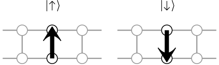
Figure 3: Schematic illustration of the states $|\!\uparrow\,\rangle$ and $|\!\downarrow\,\rangle$. The arrow denotes a state with a finite current running in the arrow’s direction.

The SF state has a long-range alternating order of $|\!\uparrow\,\rangle$ and $|\!\downarrow\,\rangle$ or, equivalently, of currents circulating around each plaquette (Fig. 4).Fjaerestad To verify the existence of the SF phase, we derive a low-energy effective theory, in perturbation expansion in $H^{\prime}$, for the low-energy states $|\!\uparrow\,\rangle_{j}$ and $|\!\downarrow\,\rangle_{j}$, which we regard as up and down states of a pseudo-spin. In this picture, the antiferromagnetic ordering of the pseudo-spins corresponds to the staggered flux phase. The lowest-order contribution in $\widetilde{H}^{\prime}$ comes from the nonvanishing matrix elements in the subspace of $|\!\uparrow\,\rangle_{j}$ and $|\!\downarrow\,\rangle_{j}$,

$$\langle\,\uparrow\!|\widetilde{H}^{\prime}|\!\uparrow\,\rangle_{j}=\langle\,\downarrow\!|\widetilde{H}^{\prime}|\!\downarrow\,\rangle_{j}\!\! = \!\!\frac{1}{2}(U+V_{\perp}-\delta t_{\mathrm{pair}}),$$ (87)

$$\langle\,\uparrow\!|\widetilde{H}^{\prime}|\!\downarrow\,\rangle_{j}=\langle\,\downarrow\!|\widetilde{H}^{\prime}|\!\uparrow\,\rangle_{j}\!\! = \!\!-\frac{1}{2}(U-V_{\perp}-\delta t_{\mathrm{pair}}),\qquad$$ (88)

from which we obtain the first-order effective Hamiltonian

$$H^{(1)}_{\mathrm{SF}}=-\frac{1}{2}\left(U-V_{\perp}-\delta t_{\mathrm{pair}}\right)\sum_{j}\tilde{\sigma}^{x}_{j}+\mathrm{const.},$$ (89)

where $\tilde{\sigma}^{a}_{j}$ are the Pauli matrices ($a=x,y,z$). The lowest-order contributions in $t_{\parallel}$ and $t_{\perp}$ come from the second-order processes,

$$H^{(2a)}_{\mathrm{SF}} = H_{t_{\parallel}}\,\frac{1}{\widetilde{E}_{0}-\widetilde{H}_{0}}\,H_{t_{\parallel}},$$ (90)

$$H^{(2b)}_{\mathrm{SF}} = H_{t_{\perp}}\,\frac{1}{\widetilde{E}_{0}-\widetilde{H}_{0}}\,H_{t_{\perp}},$$ (91)

where $\widetilde{E}_{0}=-3J_{\perp}N/4$ with $N$ being the number of rungs in the system. The nonzero matrix elements of $H^{(2a)}_{\mathrm{SF}}$ are given by

$$\langle\,\uparrow,\downarrow\!|H^{(2a)}_{\mathrm{SF}}|\!\uparrow,\downarrow\,\rangle_{j}=\langle\,\downarrow,\uparrow\!|H^{(2a)}_{\mathrm{SF}}|\!\downarrow,\uparrow\,\rangle_{j}=-\frac{8t_{\parallel}^{2}}{3J_{\perp}},$$ (92)

where $|\mu,\nu\rangle_{j}\equiv|\mu\rangle_{j}|\nu\rangle_{j+1}$ ($\mu,\nu=\uparrow,\downarrow$). We can thus write $H^{(2a)}_{\mathrm{SF}}$ as

$$H^{(2a)}_{\mathrm{SF}}=\frac{4t_{\parallel}^{2}}{3J_{\perp}}\sum_{j}\left(\tilde{\sigma}_{j}^{z}\,\tilde{\sigma}_{j+1}^{z}-1\right).$$ (93)

On the other hand, the nonzero matrix elements of $H^{(2b)}_{\mathrm{SF}}$ are

$$\langle\,\uparrow\!|H^{(2b)}_{\mathrm{SF}}|\!\uparrow\,\rangle_{j}=\langle\,\downarrow\!|H^{(2b)}_{\mathrm{SF}}|\!\downarrow\,\rangle_{j}$$

$$=\langle\,\uparrow\!|H^{(2b)}_{\mathrm{SF}}|\!\downarrow\,\rangle_{j}=\langle\,\downarrow\!|H^{(2b)}_{\mathrm{SF}}|\!\uparrow\,\rangle_{j}=-\frac{4t_{\perp}^{2}}{3J_{\perp}},\qquad$$ (94)

from which we obtain

$$H^{(2b)}_{\mathrm{SF}}=-\frac{4t_{\perp}^{2}}{3J_{\perp}}\sum_{j}\tilde{\sigma}^{x}_{j}+\mathrm{const}.$$ (95)

From Eqs. (89), (93), and (95), we find that the total effective Hamiltonian is the Ising chain in a transverse field,

$$H^{\mathrm{eff}}_{\mathrm{SF}}=\sum_{j}\left(\widetilde{K}\,\tilde{\sigma}_{j}^{z}\,\tilde{\sigma}_{j+1}^{z}-\tilde{h}\,\tilde{\sigma}_{j}^{x}\right),$$ (96)

where the antiferromagnetic exchange coupling $\widetilde{K}$ and the magnitude of the transverse field $\tilde{h}$ are given by

$$\widetilde{K}=\frac{4t_{\parallel}^{2}}{3J_{\perp}},\,\,\,\,\tilde{h}=\frac{1}{2}\left(U-V_{\perp}-\delta t_{\mathrm{pair}}+\frac{8t_{\perp}^{2}}{3J_{\perp}}\right).$$ (97)

This model exhibits an Ising criticality at $\widetilde{K}=|\tilde{h}|$: the Néel ordered phase ($\widetilde{K}>|\tilde{h}|$) corresponds to the SF phase, while for $\widetilde{K}<|\tilde{h}|$ the system is disordered. The disordered ground state for $\tilde{h}>\widetilde{K}>0$ is continuously connected with the ground state at $\tilde{h}\to\infty$, i.e., the eigenstate of $\tilde{\sigma}^{x}$ with eigenvalue $+1$. This state corresponds to the D-Mott state in the original Hubbard ladder, since

$$|{\tilde{\sigma}^{x}\!=+1}\rangle_{j} \!\!=\!\! \frac{1}{\sqrt{2}}\left(|\!\uparrow\,\rangle_{j}+|\!\downarrow\,\rangle_{j}\right)$$ (98)

$$\!\!=\!\! \frac{1}{\sqrt{2}}\left(|1\rangle_{j}-|2\rangle_{j}\right)\to|\mbox{D-Mott}\rangle.$$

Hence we conclude that the Ising disordered phase corresponds to the D-Mott phase.

Figure 4: Staggered flux state described as a Néel ordered state of the pseudo-spin states, $|\!\uparrow\,\rangle$ and $|\!\downarrow\,\rangle$.

It is interesting to rewrite the transverse magnetic field $\tilde{h}$ as

$$\tilde{h} = \frac{1}{2}\left(U-V_{\perp}+\frac{3}{4}J_{\perp}-t_{\mathrm{pair}}+\frac{8t_{\perp}^{2}}{3J_{\perp}}\right).$$ (99)

The SF phase is realized when the inequality

$$-\frac{16t^{2}}{3J_{\perp}}<U-V_{\perp}+\frac{3}{4}J_{\perp}-t_{\mathrm{pair}}<0$$ (100)

is satisfied (assuming $t_{\parallel}=t_{\perp}=t$), where we have to keep in mind the assumption that $t_{\mathrm{pair}}\approx\frac{3}{4}J_{\perp}$.

IV Weak-Coupling Approach

In this section, we study the phase diagram of the generalized Hubbard ladder, treating the two-particle interactions as weak perturbations. To diagonalize the single-particle hopping Hamiltonian, we define the Fourier transform, $c_{j,\sigma}({k_{\perp}\!=\!0})=(c_{j,1,\sigma}+c_{j,2,\sigma})/\sqrt{2}$, $c_{j,\sigma}({k_{\perp}\!=\!\pi})=(c_{j,1,\sigma}-c_{j,2,\sigma})/\sqrt{2}$, and $c_{\sigma}(\bm{k})=\sum_{j}e^{-ikj}c_{j,\sigma}(k_{\perp})/\sqrt{N}$, where $\bm{k}=(k,k_{\perp})$ and the lattice spacing $a$ is set equal to 1. The kinetic energy term then becomes

$$H_{0}\equiv H_{t_{\parallel}}+H_{t_{\perp}}=\sum_{\bm{k},\sigma}\varepsilon(\bm{k})\,c_{\sigma}^{\dagger}(\bm{k})\,c_{\sigma}(\bm{k}),$$ (101)

where $\varepsilon(\bm{k})=-2t_{\parallel}\cos k-t_{\perp}\cos k_{\perp}$. For $t_{\perp}<2t_{\parallel}$, both the bonding ($k_{\perp}=0$) and antibonding ($k_{\perp}=\pi$) energy bands are partially filled, and their Fermi points are located at $k=\pm k_{F,k_{\perp}}$ with $k_{F,0}=\frac{\pi}{2}+\delta$ and $k_{F,\pi}=\frac{\pi}{2}-\delta$, where $\delta\equiv\sin^{-1}(t_{\perp}/2t_{\parallel})$. At these Fermi points the Fermi velocity takes the common value $v_{F}=2t_{\parallel}[1-(t_{\perp}/2t_{\parallel})^{2}]^{1/2}$. In the following analysis we restrict ourselves to the isotropic hopping case $t_{\parallel}=t_{\perp}(\equiv t)$.

IV.1 Order parameters

Let us first define order parameters characterizing insulating phases studied in this section. We consider the CDW, SF, $p$-density-wave (PDW), and $f$-density-wave (FDW) states as possible density-wave ordered states. Their order parameters are written as

$$O_{\mathrm{A}}\!\! = \!\!\frac{1}{2N}\sum_{\bm{k},\sigma}f_{\mathrm{A}}(\bm{k})\,c_{\sigma}^{\dagger}(\bm{k})\,c_{\sigma}(\bm{k}+\bm{Q})$$ (102)

$$\equiv \!\!\frac{1}{N}\sum_{j}(-1)^{j}\mathcal{O}_{\mathrm{A}}(j),$$

where $\bm{Q}=(\pi,\pi)$ and A = CDW, SF, PDW, FDW. The form factor $f_{\mathrm{A}}(\bm{k})$ are given by $f_{\mathrm{CDW}}=1$, $f_{\mathrm{SF}}=\cos k-\cos k_{\perp}$, $f_{\mathrm{PDW}}=\sin k$, and $f_{\mathrm{FDW}}=\sin k\,\cos k_{\perp}$. Order parameters for the spin density waves are not considered, since their correlations decay exponentially in the bulk of the phase diagram of our model. It is clear that the CDW order parameter,

$$\mathcal{O}_{\mathrm{CDW}}=\frac{1}{2}(n_{j,1}-n_{j,2}),$$ (103)

has nonvanishing average in the CDW states (33a) and (33b). The order parameter of the SF state is

$$\mathcal{O}_{\mathrm{SF}}=\frac{1}{4i}\hat{J}_{\mathrm{P},j},$$ (104)

where the operator $\hat{J}_{\mathrm{P},j}$ denotes a current circulating around a plaquette:

$$\hat{J}_{\mathrm{P},j}\!\! \equiv \!\!i\sum_{\sigma}\Bigl{(}c_{j,1,\sigma}^{\dagger}\,c_{j,2,\sigma}+c_{j,2,\sigma}^{\dagger}\,c_{j+1,2,\sigma}$$ (105)

$${}+c_{j+1,2,\sigma}^{\dagger}\,c_{j+1,1,\sigma}+c_{j+1,1,\sigma}^{\dagger}\,c_{j,1,\sigma}-\mathrm{H.c.}\Bigr{)}.\qquad$$

The PDW phase is a Peierls dimerized state along the leg direction with inter-leg phase difference $\pi$, characterized by the order parameter,

$$\mathcal{O}_{\mathrm{PDW}}=\frac{i}{4}\sum_{\sigma}\biggl{(}c_{j+1,1,\sigma}^{\dagger}\,c_{j,1,\sigma}-c_{j+1,2,\sigma}^{\dagger}\,c_{j,2,\sigma}+\mathrm{H.c.}\biggr{)}.$$ (106)

The FDW state is a different kind of staggered current states. Its order parameter is

$$\mathcal{O}_{\mathrm{FDW}}=\frac{1}{4}\left(\hat{J}_{+,j}-\hat{J}_{-,j}\right),$$ (107)

where the operators $\hat{J}_{\pm,j}$ represent currents flowing along the diagonal directions of plaquettes:

$$\hat{J}_{+,j}\!\! = \!\!i\sum_{\sigma}\left(c^{\dagger}_{j+1,2,\sigma}c_{j,1,\sigma}-c^{\dagger}_{j,1,\sigma}c_{j+1,2,\sigma}\right),$$ (108)

$$\hat{J}_{-,j}\!\! = \!\!i\sum_{\sigma}\left(c^{\dagger}_{j+1,1,\sigma}c_{j,2,\sigma}-c^{\dagger}_{j,2,\sigma}c_{j+1,1,\sigma}\right).$$ (109)

The long-range order of staggered currents flowing along diagonals of the plaquettes has been examined in a spinless ladder system.Nersesyan1991

We also introduce order parameters of the $s$-wave and $d$-wave superconductivity,

$$O_{\mathrm{A}}=\frac{1}{2N}\sum_{\bm{k}}f_{\mathrm{A}}(\bm{k})\,c_{\uparrow}(\bm{k})\,c_{\downarrow}(-\bm{k}),$$ (110)

where A = SCs and SCd, and $f_{\mathrm{SCs}}=1$ and $f_{\mathrm{SCd}}=\cos k-\cos k_{\perp}$.

IV.2 Bosonization

We bosonize the Hubbard ladder Hamiltonian in this subsection. Following the standard bosonization scheme, we linearize the energy bands around the Fermi points. The linearized kinetic energy is given by

$$H_{0}=\sum_{\bm{k},p,\sigma}v_{F}(pk-k_{F,k_{\perp}})\,c_{p,\sigma}^{\dagger}(\bm{k})\,c_{p,\sigma}(\bm{k}),$$ (111)

where the index $p=+/-$ denotes the right/left-moving electron. We introduce field operators of the right- and left-going electrons defined by

$$\psi_{p,\sigma,+}(x)\!\! = \!\!\frac{1}{\sqrt{L}}\sum_{k}e^{ikx}c_{p,\sigma}(k,0),$$ (112a)

$$\psi_{p,\sigma,-}(x)\!\! = \!\!\frac{1}{\sqrt{L}}\sum_{k}e^{ikx}c_{p,\sigma}(k,\pi),$$ (112b)

where $L$ is the length of the system: $L=Na$. The linearized kinetic energy now reads

$$H_{0}=v_{F}\int dx\sum_{p,\sigma,\zeta}\psi^{\dagger}_{p,\sigma,\zeta}\left(-ip\frac{d}{dx}-k_{F,k_{\perp}}\right)\psi_{p,\sigma,\zeta},$$ (113)

where $k_{\perp}=0$ ($\pi$) for $\zeta=+$ ($-$).

The interactions among low-energy excitations near the Fermi points, $H_{I}=H_{\mathrm{int}}+H_{V_{\parallel}}+H_{V^{\prime}}+H_{\mathrm{pair}}$, are written as $H_{I}=\int dx\mathcal{H}_{I}$, where

$$\mathcal{H}_{I} \!\!=\!\! \frac{1}{4}\sum_{p,\sigma}{\sum_{\zeta_{i}=\pm}}^{\prime}\biggl{[}g_{1\parallel}^{\epsilon\bar{\epsilon}}\,\psi_{p,\sigma,\zeta_{1}}^{\dagger}\,\psi_{-p,\sigma,\zeta_{2}}^{\dagger}\,\psi_{p,\sigma,\zeta_{4}}\,\psi_{-p,\sigma,\zeta_{3}}$$

$$\hskip 36.98857pt{}+g_{1\perp}^{\epsilon\bar{\epsilon}}\,\psi_{p,\sigma,\zeta_{1}}^{\dagger}\,\psi_{-p,-\sigma,\zeta_{2}}^{\dagger}\,\psi_{p,-\sigma,\zeta_{4}}\,\psi_{-p,\sigma,\zeta_{3}}$$

$$\hskip 36.98857pt{}+g_{2\parallel}^{\epsilon\bar{\epsilon}}\,\psi_{p,\sigma,\zeta_{1}}^{\dagger}\,\psi_{-p,\sigma,\zeta_{2}}^{\dagger}\,\psi_{-p,\sigma,\zeta_{4}}\,\psi_{p,\sigma,\zeta_{3}}$$

$$\hskip 36.98857pt{}+g_{2\perp}^{\epsilon\bar{\epsilon}}\,\psi_{p,\sigma,\zeta_{1}}^{\dagger}\,\psi_{-p,-\sigma,\zeta_{2}}^{\dagger}\,\psi_{-p,-\sigma,\zeta_{4}}\,\psi_{p,\sigma,\zeta_{3}}$$

$$\hskip 36.98857pt{}+g_{3\parallel}^{\epsilon\bar{\epsilon}}\,\psi_{p,\sigma,\zeta_{1}}^{\dagger}\,\psi_{p,\sigma,\zeta_{2}}^{\dagger}\,\psi_{-p,\sigma,\zeta_{4}}\,\psi_{-p,\sigma,\zeta_{3}}$$

$$\hskip 36.98857pt{}+g_{3\perp}^{\epsilon\bar{\epsilon}}\,\psi_{p,\sigma,\zeta_{1}}^{\dagger}\,\psi_{p,-\sigma,\zeta_{2}}^{\dagger}\,\psi_{-p,-\sigma,\zeta_{4}}\,\psi_{-p,\sigma,\zeta_{3}}\biggr{]}.$$

Here $\epsilon=\zeta_{1}\zeta_{3}$ and $\bar{\epsilon}=\zeta_{1}\zeta_{2}$. The primed summation over $\zeta_{i}$ ($i=1,\ldots,4$) is taken under the condition $\zeta_{1}\zeta_{2}\zeta_{3}\zeta_{4}=+1$, which comes from the momentum conservation condition in the transverse direction. The coupling constants $g_{i\parallel}^{\epsilon\bar{\epsilon}}$ and $g_{i\perp}^{\epsilon\bar{\epsilon}}$ are related to the original coupling constants in the Hamiltonian (1):

$$\frac{g_{i\parallel}^{\epsilon\bar{\epsilon}}}{a}\!\! = \!\!l_{\epsilon}V_{\perp}+\frac{l_{\epsilon}}{4}J_{\perp}+m_{i,\epsilon}V_{\parallel}+l_{\epsilon}m_{i,\epsilon}V^{\prime},$$ (115)

$$\frac{g_{i\perp}^{\epsilon\bar{\epsilon}}}{a}\!\! = \!\!U+l_{\epsilon}V_{\perp}+\frac{l_{\epsilon,\bar{\epsilon}}}{4}J_{\perp}+l_{\bar{\epsilon}}t_{\mathrm{pair}}+m_{i,\epsilon}V_{\parallel}+l_{\epsilon}m_{i,\epsilon}V^{\prime}$$

with the numerical factors defined by $l_{\pm}=\pm 1$, $l_{\pm,+}=\mp 3$, $l_{\pm,-}=\pm 1$. $m_{1,+}=m_{3,+}=-1$, $m_{1,-}=m_{3,-}=-2$, $m_{2,+}=+2$, $m_{2,-}=+1$. We have neglected the so-called $g_{4}$ terms describing the forward scattering processes within the same branch (left-/right-mover), since including these terms would only cause nonuniversal quantitative differences to the ground state phase diagram. In Eqs. (115) and (LABEL:eq:gperp), we have estimated the coupling constants in lowest order in the interaction of the Hubbard model. The higher-order contributions can play a crucial role of changing topology of a phase diagram, if different kinds of quantum criticalities accidentally occur simultaneously when lowest-order coupling constants are used, as is the case in the 1D extended Hubbard model at half-filling.Tsuchiizu2002 This is not the case in the ladder model of our interest, and we will use the lowest order form, Eqs. (115) and (LABEL:eq:gperp).

We apply the Abelian bosonization methodEmery ; Solyom ; Gogolin_book and rewrite the kinetic energy in terms of bosonic fields: $H_{0}=\int dx\mathcal{H}_{0}$, where

$${\cal H}_{0}=\frac{v_{F}}{2\pi}\sum_{\nu=\rho,\sigma}\sum_{r=\pm}\left[\left(\pi\Pi_{\nu r}\right)^{2}+\left(\frac{d\phi_{\nu r}}{dx}\right)^{2}\right].$$ (117)

Here the suffices $\rho$ and $\sigma$ refer to the charge and spin sectors and $r=\pm$ refer to the even and odd sectors. The operator $\Pi_{\nu r}(x)$ is a canonically conjugate variable to $\phi_{\nu r}(x)$ and satisfies $[\phi_{\nu r}(x),\Pi_{\nu^{\prime}r^{\prime}}(x^{\prime})]=i\,\delta(x-x^{\prime})\,\delta_{\nu,\nu^{\prime}}\,\delta_{r,r^{\prime}}$. We then introduce chiral bosonic fields

$$\phi_{\nu r}^{\pm}(x)\equiv\frac{1}{2}\left[\phi_{\nu r}(x)\mp\pi\int_{-\infty}^{x}dx^{\prime}\,\Pi_{\nu r}(x^{\prime})\right],$$ (118)

which satisfy the commutation relations $[\phi_{\nu r}^{\pm}(x),\phi_{\nu^{\prime}r^{\prime}}^{\pm}(x^{\prime})]=\pm i(\pi/4)\,\mathrm{sgn}(x-x^{\prime})\,\delta_{\nu,\nu^{\prime}}\,\delta_{r,r^{\prime}}$ and $[\phi_{\nu r}^{+}(x),\phi_{\nu^{\prime}r^{\prime}}^{-}(x^{\prime})]=i(\pi/4)\,\delta_{\nu,\nu^{\prime}}\,\delta_{r,r^{\prime}}$. The right-moving and left-moving chiral fields $\phi^{+}(x,\tau)$ and $\phi^{-}(x,\tau)$ are functions of $\tau-i(x/v_{F})$ and $\tau+i(x/v_{F})$, respectively, where $\tau$ is imaginary time. The kinetic-energy density can also be written as

$${\cal H}_{0}=\frac{v_{F}}{\pi}\sum_{p=\pm}\sum_{\nu=\rho,\sigma}\sum_{r=\pm}\left(\frac{d\phi_{\nu r}^{p}}{dx}\right)^{2}.$$ (119)

We also introduce the field $\theta_{\nu r}$ defined by $\theta_{\nu r}=\phi_{\nu r}^{+}-\phi_{\nu r}^{-}$. The $\theta$ field satisfies the commutation relation $[\phi_{\nu r}(x),\theta_{\nu^{\prime}r^{\prime}}(x^{\prime})]=-i\pi\Theta(-x+x^{\prime})\delta_{r,r^{\prime}}$, where $\Theta(x)$ is the Heaviside step function.

To express the electron fields in terms of the bosons, we define a new set of chiral bosonic fields

$$\varphi_{p,s,\zeta}=\phi_{\rho+}^{p}+\zeta\phi_{\rho-}^{p}+s\phi_{\sigma+}^{p}+s\zeta\phi_{\sigma-}^{p},$$ (120)

where $p=\pm$, $s=\pm$, and $\zeta=\pm$. The chiral bosons obey the commutation relations $[\varphi_{p,s,\zeta}(x),\varphi_{p,s^{\prime},\zeta^{\prime}}(x^{\prime})]$ $=ip\pi\,\mathrm{sgn}(x-x^{\prime})\,\delta_{s,s^{\prime}}\,\delta_{\zeta,\zeta^{\prime}}$ and $[\varphi_{+,s,\zeta},\varphi_{-,s^{\prime},\zeta^{\prime}}]=i\pi\,\delta_{s,s^{\prime}}\,\delta_{\zeta,\zeta^{\prime}}$.

The field operators of the right- and left-moving electrons are then written as

$$\psi_{p,\sigma,\zeta}=\frac{\eta_{\sigma,\zeta}}{\sqrt{2\pi a}}\exp\left(ipk_{F,k_{\perp}}x+ip\,\varphi_{p,s,\zeta}\right),$$ (121)

where $s=+$ for $\sigma=\uparrow$ and $s=-$ for $\sigma=\downarrow$. The Klein factors $\eta_{\sigma,\zeta}$, which satisfy $\{\eta_{\sigma,\zeta},\eta_{\sigma^{\prime},\zeta^{\prime}}\}=2\delta_{\sigma,\sigma^{\prime}}\delta_{\zeta,\zeta^{\prime}}$, are introduced in order to retain the correct anticommutation relation of the field operators between different spin and the band index. From Eq. (121) the density operator is given by

$$\rho_{p,\sigma,\zeta}(x)=\,:\!\psi_{p,\sigma,\zeta}^{\dagger}\,\psi_{p,\sigma,\zeta}\!:\,=\,\frac{1}{2\pi}\,\frac{d}{dx}\varphi_{p,s,\zeta}(x).$$ (122)

The Hamiltonian and the order parameters contain only products of the Klein factors such asSchulz1996 ; Fjaerestad $\Gamma\equiv\eta_{\uparrow,+}\,\eta_{\downarrow,+}\,\eta_{\uparrow,-}\,\eta_{\downarrow,-}$, $h_{\sigma}\equiv\eta_{\sigma,+}\,\eta_{\sigma,-}$, and $h^{\prime}_{\zeta}\equiv\eta_{\uparrow,\zeta}\,\eta_{\downarrow,\zeta}$, which satisfy $\Gamma=-h_{\uparrow}\,h_{\downarrow}=+h^{\prime}_{+}\,h^{\prime}_{-}$. Since $\Gamma^{2}=+1$, $h^{2}=(h^{\prime})^{2}=-1$, the eigenvalues are $\Gamma=\pm 1$, $h=\pm i$, and $h^{\prime}=\pm i$. We will adopt the following convention: $\Gamma=+1$, $h_{\sigma}=i$, $h_{\zeta}^{\prime}=i\zeta$.

In the bosonized Hamiltonian the phase field $\phi_{\rho-}$ appears in the form $\cos(2\phi_{\rho-}+4\delta x)$ with $\delta=\sin^{-1}(t_{\perp}/2t_{\parallel})$. Since $t_{\perp}$ $(=t_{\parallel})$ is not small, we can safely assume that the $\delta$ is relevant and the electrons are not confined in the legs. Tsuchiizu1999 ; LeHur ; Tsuchiizu2001 In this case the $\cos(2\phi_{\rho-}+4\delta x)$ terms become irrelevant. We thus discard them as well as other terms with higher-order scaling dimensions. The interaction term Eq. (LABEL:eq:Hint_g-ology) reduces to

$$\mathcal{H}_{I} \!\!=\!\! \sum_{\nu=\rho,\sigma}\sum_{r=\pm}\frac{g_{\nu r}}{2\pi^{2}}\left(\partial_{x}\phi_{\nu r}^{+}\right)\left(\partial_{x}\phi_{\nu r}^{-}\right)$$ (123)

$$\!\!{}+\frac{1}{2\pi^{2}a^{2}}\Bigl{[}g_{c+,\overline{c-}}\,\cos 2\phi_{\rho+}\,\cos 2\theta_{\rho-}$$

$${}+g_{c+,s+}\,\cos 2\phi_{\rho+}\,\cos 2\phi_{\sigma+}$$

$${}+g_{c+,s-}\,\cos 2\phi_{\rho+}\,\cos 2\phi_{\sigma-}$$

$${}+g_{c+,\overline{s-}}\,\cos 2\phi_{\rho+}\,\,\cos 2\theta_{\sigma-}$$

$${}+g_{\overline{c-},s+}\,\cos 2\theta_{\rho-}\,\cos 2\phi_{\sigma+}$$

$${}+g_{\overline{c-},s-}\,\cos 2\theta_{\rho-}\,\cos 2\phi_{\sigma-}$$

$${}+g_{\overline{c-},\overline{s-}}\,\cos 2\theta_{\rho-}\,\,\cos 2\theta_{\sigma-}$$

$${}+g_{s+,s-}\,\cos 2\phi_{\sigma+}\,\cos 2\phi_{\sigma-}$$

$${}+g_{s+,\overline{s-}}\,\cos 2\phi_{\sigma+}\,\cos 2\theta_{\sigma-}\Bigr{]},$$

where the coupling constants for the bilinear terms of the density operators are given by

$$g_{\rho+}\!\! = \!\!\sum_{\epsilon=\pm}(g_{2\parallel}^{+\epsilon}+g_{2\perp}^{+\epsilon}-g_{1\parallel}^{\epsilon\epsilon}),$$ (124a)

$$g_{\rho-}\!\! = \!\!\sum_{\epsilon=\pm}\epsilon(g_{2\parallel}^{+\epsilon}+g_{2\perp}^{+\epsilon}-g_{1\parallel}^{\epsilon\epsilon}),$$ (124b)

$$g_{\sigma+}\!\! = \!\!\sum_{\epsilon=\pm}(g_{2\parallel}^{+\epsilon}-g_{2\perp}^{+\epsilon}-g_{1\parallel}^{\epsilon\epsilon}),$$ (124c)

$$g_{\sigma-}\!\! = \!\!\sum_{\epsilon=\pm}\epsilon(g_{2\parallel}^{+\epsilon}-g_{2\perp}^{+\epsilon}-g_{1\parallel}^{\epsilon\epsilon}),$$ (124d)

and the coupling constants for the nonlinear terms are given by

$$g_{c+,\overline{c-}}\!\! = \!\!-g_{3\perp}^{-+},$$ (125a)

$$g_{c+,s+}\!\! = \!\!-g_{3\parallel}^{+-}+g_{3\parallel}^{--},$$ (125b)

$$g_{c+,s-}\!\! = \!\!-g_{3\perp}^{+-},$$ (125c)

$$g_{c+,\overline{s-}}\!\! = \!\!+g_{3\perp}^{--},$$ (125d)

$$g_{\overline{c-},s+}\!\! = \!\!-g_{1\perp}^{-+},$$ (125e)

$$g_{\overline{c-},s-}\!\! = \!\!-g_{2\perp}^{-+},$$ (125f)

$$g_{\overline{c-},\overline{s-}}\!\! = \!\!+g_{2\parallel}^{-+}-g_{1\parallel}^{-+},$$ (125g)

$$g_{s+,s-}\!\! = \!\!+g_{1\perp}^{++},$$ (125h)

$$g_{s+,\overline{s-}}\!\! = \!\!+g_{1\perp}^{--}.$$ (125i)

We note that the umklapp scattering (the $g_{3}$ terms) generates cosine potentials that lock the $\phi_{\rho+}$ field.

The coupling constants in Eq. (123) are not independent parameters. Imposing the global spin-rotation SU(2) symmetry on the interaction terms Eq. (LABEL:eq:Hint_g-ology), we find that the relations

$$g_{2\parallel}^{++}-g_{2\perp}^{++}-g_{1\parallel}^{++}+g_{1\perp}^{++}=0,$$ (126a)

$$g_{2\parallel}^{+-}-g_{2\perp}^{+-}-g_{1\parallel}^{--}+g_{1\perp}^{--}=0,$$ (126b)

$$g_{2\parallel}^{--}-g_{2\perp}^{--}-g_{1\parallel}^{+-}+g_{1\perp}^{+-}=0,$$ (126c)

$$g_{2\parallel}^{-+}-g_{2\perp}^{-+}-g_{1\parallel}^{-+}+g_{1\perp}^{-+}=0,$$ (126d)

$$g_{3\parallel}^{+-}-g_{3\parallel}^{--}-g_{3\perp}^{+-}+g_{3\perp}^{--}=0,$$ (126e)

must hold. In terms of the coupling constants in Eq. (123), these relations read

$$g_{\sigma+}+g_{\sigma-}+2g_{s+,s-}=0,$$ (127a)

$$g_{\sigma+}-g_{\sigma-}+2g_{s+,\overline{s-}}=0,$$ (127b)

$$g_{\overline{c-},s+}-g_{\overline{c-},s-}-g_{\overline{c-},\overline{s-}}=0,$$ (127c)

$$g_{c+,s+}-g_{c+,s-}-g_{c+,\overline{s-}}=0.$$ (127d)

We have ignored Eq. (126c) which is the constraint on the irrelevant cosine term $\propto\cos(2\phi_{\rho-}+4\delta x)$. Since the SU(2) symmetry of the original Hubbard Hamiltonian (1) cannot be broken, the coupling constants in Eq. (123) must satisfy Eqs. (127a)-(127d) in the course of renormalization.

Finally, the order parameters are written in terms of the phase fields:

$$\mathcal{O}_{\mathrm{CDW}}\propto\cos\phi_{\rho+}\,\sin\theta_{\rho-}\,\cos\phi_{\sigma+}\,\cos\theta_{\sigma-}$$

$$\qquad\qquad{}-\sin\phi_{\rho+}\,\cos\theta_{\rho-}\,\sin\phi_{\sigma+}\,\sin\theta_{\sigma-},$$ (128a)

$$\mathcal{O}_{\mathrm{SF}}\propto\cos\phi_{\rho+}\,\cos\theta_{\rho-}\,\cos\phi_{\sigma+}\,\cos\theta_{\sigma-}$$

$$\qquad\quad{}+\sin\phi_{\rho+}\,\sin\theta_{\rho-}\,\sin\phi_{\sigma+}\,\sin\theta_{\sigma-},$$ (128b)

$$\mathcal{O}_{\mathrm{PDW}}\propto\cos\phi_{\rho+}\,\cos\theta_{\rho-}\,\sin\phi_{\sigma+}\,\sin\theta_{\sigma-}$$

$$\qquad\qquad{}+\sin\phi_{\rho+}\,\sin\theta_{\rho-}\,\cos\phi_{\sigma+}\,\cos\theta_{\sigma-},$$ (128c)

$$\mathcal{O}_{\mathrm{FDW}}\propto\cos\phi_{\rho+}\,\sin\theta_{\rho-}\,\sin\phi_{\sigma+}\,\sin\theta_{\sigma-}$$

$$\qquad\qquad{}-\sin\phi_{\rho+}\,\cos\theta_{\rho-}\,\cos\phi_{\sigma+}\,\cos\theta_{\sigma-}.\qquad\quad$$ (128d)

$$\mathcal{O}_{\mathrm{SCd}}\propto e^{i\theta_{\rho+}}\cos\theta_{\rho-}\,\cos\phi_{\sigma+}\,\cos\phi_{\sigma-}$$

$$\qquad\qquad{}-i\,e^{i\theta_{\rho+}}\sin\theta_{\rho-}\,\sin\phi_{\sigma+}\,\sin\phi_{\sigma-},$$ (128e)

$$\mathcal{O}_{\mathrm{SCs}}\propto e^{i\theta_{\rho+}}\cos\theta_{\rho-}\,\sin\phi_{\sigma+}\,\sin\phi_{\sigma-}$$

$$\qquad\qquad{}-i\,e^{i\theta_{\rho+}}\sin\theta_{\rho-}\,\cos\phi_{\sigma+}\,\cos\phi_{\sigma-}.$$ (128f)

IV.3 Critical properties in the charge and spin modes

In this subsection, we study the ground state phase diagram through qualitative analysis of the bosonized Hamiltonian (123). First we classify the phases that can appear at half-filling, and then discuss (a) the Gaussian criticality in the charge sector and (b) the Ising and SU(2)₂ criticalities in the spin sector.

IV.3.1 Classification of phases

Table 1: Pattern of phase locking. The $*$ symbol indicates that a bosonic field is not locked. $I_{i}$s are integers.

Phase	$\langle\phi_{\rho+}\rangle$	$\langle\theta_{\rho-}\rangle$	$\langle\phi_{\sigma+}\rangle$	$\langle\phi_{\sigma-}\rangle$	$\langle\theta_{\sigma-}\rangle$
CDW	$\frac{\pi}{2}I_{0}+\pi I_{1}$	$\frac{\pi}{2}(I_{0}+1)+\pi I_{2}$	$\frac{\pi}{2}I_{0}+\pi I_{3}$	$*$	$\frac{\pi}{2}I_{0}+\pi I_{4}$
SF	$\frac{\pi}{2}I_{0}+\pi I_{1}$	$\frac{\pi}{2}I_{0}+\pi I_{2}$	$\frac{\pi}{2}I_{0}+\pi I_{3}$	$*$	$\frac{\pi}{2}I_{0}+\pi I_{4}$
PDW	$\frac{\pi}{2}(I_{0}+1)+\pi I_{1}$	$\frac{\pi}{2}(I_{0}+1)+\pi I_{2}$	$\frac{\pi}{2}I_{0}+\pi I_{3}$	$*$	$\frac{\pi}{2}I_{0}+\pi I_{4}$
FDW	$\frac{\pi}{2}(I_{0}+1)+\pi I_{1}$	$\frac{\pi}{2}I_{0}+\pi I_{2}$	$\frac{\pi}{2}I_{0}+\pi I_{3}$	$*$	$\frac{\pi}{2}I_{0}+\pi I_{4}$
S-Mott	$\frac{\pi}{2}I_{0}+\pi I_{1}$	$\frac{\pi}{2}(I_{0}+1)+\pi I_{2}$	$\frac{\pi}{2}I_{0}+\pi I_{3}$	$\frac{\pi}{2}I_{0}+\pi I_{4}$	$*$
D-Mott	$\frac{\pi}{2}I_{0}+\pi I_{1}$	$\frac{\pi}{2}I_{0}+\pi I_{2}$	$\frac{\pi}{2}I_{0}+\pi I_{3}$	$\frac{\pi}{2}I_{0}+\pi I_{4}$	$*$
S’-Mott	$\frac{\pi}{2}(I_{0}+1)+\pi I_{1}$	$\frac{\pi}{2}(I_{0}+1)+\pi I_{2}$	$\frac{\pi}{2}I_{0}+\pi I_{3}$	$\frac{\pi}{2}I_{0}+\pi I_{4}$	$*$
D’-Mott	$\frac{\pi}{2}(I_{0}+1)+\pi I_{1}$	$\frac{\pi}{2}I_{0}+\pi I_{2}$	$\frac{\pi}{2}I_{0}+\pi I_{3}$	$\frac{\pi}{2}I_{0}+\pi I_{4}$	$*$

In general all the modes become massive in the extended Hubbard ladder at half-filling. This means that in the bosonized Hamiltonian (123) cosine terms are relevant at low energies and that the bosonic phase fields are locked at some fixed values (integer multiples of $\pi/2$) where the relevant cosine potentials are minimized.Lin The locked phase fields can be treated as classical variables, and the average value of an order parameter is found by substituting the locked phases into Eq. (128). A nonvanishing order parameter signals which phase is realized. We can reverse the logic and find the configuration of the locked phase fields for each insulating phase by imposing its order parameter to have its maximum modulus. This is what we do in the following analysis.

In the SF, CDW, PDW, and FDW phases the ground state breaks a Z₂ symmetry. Therefore the order parameter of these phases can have a nonvanishing value at zero temperature even in one dimension. In each phase the bosonic fields $\phi_{\rho+}$, $\theta_{\rho-}$, $\phi_{\sigma+}$, and $\theta_{\sigma-}$ are pinned at a point where the modulus of the corresponding order parameter is maximized. From Eq. (128) we can easily find at which values the bosonic fields are locked for the four phases. The result is summarized in Table 1.

Once the configuration of locked phase fields is understood for the SF and the CDW phases, we can also find that for the D-Mott and the S-Mott phases using the following arguments. On the one hand, we know from the strong-coupling analysis that these two insulating phases are Ising disordered phases of the SF and the CDW phases, respectively, where the $\theta_{\sigma-}$ field is locked. On the other hand, the Hamiltonian (123) has some cosine potentials that can lock the $\phi_{\sigma-}$ field. Since the $\phi_{\sigma-}$ field is a conjugate field to $\theta_{\sigma-}$, these two fields cannot be locked at the same time. In fact, it is known Schulz1996 that an Ising phase transition must be associated with switching of phase locking from one bosonic field to its conjugate field. We can thus obtain the D-Mott and the S-Mott phases from the SF and the CDW phases by exchanging the role of the $\phi_{\sigma-}$ field and the $\theta_{\sigma-}$ field, arriving at the phase locking pattern shown in Table 1. A brief comment on the connection to the superconducting states is in order here. If we ignore the $\rho+$ mode for the moment, the order parameter of the $d$-wave ($s$-wave) superconductivity takes nonzero amplitude when the locked phases ($\langle\theta_{\rho-}\rangle$, $\langle\phi_{\sigma+}\rangle$, and $\langle\phi_{\sigma-}\rangle$) of the D-Mott (S-Mott) phase are substituted into $\mathcal{O}_{\mathrm{SCd(s)}}$. This is consistent with the previous resultsFabrizio ; Noack ; Sigrist ; Tsunetsugu1994 ; Khveshchenko1994 ; Nagaosa ; Dagotto ; Schulz1996 ; Balents1996 ; Orignac ; Tsuchiizu2001 that, upon doping, the D-Mott state turns into the $d$-wave superconducting state in the $t$-$J$ or Hubbard ladder. The effect of carrier doping is to make the umklapp term irrelevant and to leave the $\phi_{\rho+}$ field unlocked. The operator $e^{i\theta_{\rho+}}$ representing the superconducting correlation then becomes quasi-long-range ordered.

It is possible to construct a disorder parameter that characterizes the Ising transitions and that has a nonvanishing expectation value in the D-Mott and the S-Mott phases. A candidate operator for the disorder parameter is

$$\mu_{j}\!\! = \!\!\exp\left(i\frac{\pi}{2}\sum_{i=1}^{j}X_{i}\right),$$

$$X_{i}\!\! = \!\!c_{i,1,\uparrow}^{\dagger}c_{i,2,\uparrow}+c_{i,2,\uparrow}^{\dagger}c_{i,1,\uparrow}$$ (129)

$${}-c_{i,1,\downarrow}^{\dagger}c_{i,2,\downarrow}-c_{i,2,\downarrow}^{\dagger}c_{i,1,\downarrow}.$$

In the weak-coupling limit we take the continuum limit and express the operator (129) in terms of the bosonic fields. We then obtain

$$\mu_{j}=\exp[i\phi_{\sigma-}(j)].$$ (130)

Indeed, the disorder parameter $\mu_{j}$ takes a nonzero value in the D-Mott and the S-Mott phases where the $\phi_{\sigma-}$ field is locked. In the strong-coupling limit studied in Sec. III, we may impose the condition that $n_{i,1}+n_{i,2}=2$ and $S^{z}_{i,1}+S^{z}_{i,2}=0$ on every rung. Under this condition we find that $\exp(i\frac{\pi}{2}X_{i})=1-\frac{1}{2}X_{i}^{2}$ and $\mu_{j}$ reduces to

$$\mu_{j}\!\! = \!\!\prod^{j}_{i=1}\biggl{[}\left(c^{\dagger}_{i,1,\uparrow}c^{\dagger}_{i,1,\downarrow}c_{i,2,\downarrow}c_{i,2,\uparrow}+\mathrm{H.c.}\right)$$ (131)

$$\quad-\left(S^{+}_{i,1}S^{-}_{i,2}+S^{-}_{i,1}S^{+}_{i,2}\right)\biggr{]},$$

which acts on the pseudo-spin states defined in Secs. IIIA and IIIC as $\mu_{j}|+\rangle_{i}=|-\rangle_{i}$ and $\mu_{j}|\!\!\!\uparrow\,\rangle_{i}=|\!\!\!\downarrow\,\rangle_{i}$ for $i\leq j$. This means that we can write $\mu_{j}=\prod^{j}_{i}\tau^{x}_{i}$ and $\mu_{j}=\prod^{j}_{i}\tilde{\sigma}^{x}_{i}$ near the CDW–S-Mott and the SF–D-Mott transitions, respectively. They are indeed the disorder parameter of the quantum Ising modelGogolin_book that describes the CDW–S-Mott and the SF–D-Mott Ising transitions.

Since the PDW and the FDW phases break Z₂ symmetry, we can naturally expect that these two phases should also have their own Ising disordered phases. We shall call them S’-Mott and D’-Mott phases for the reason that will become clear below. The configuration of phase locking in the S’-Mott and D’-Mott phases can be obtained from that of the PDW and FDW phases by exchanging $\langle\phi_{\sigma-}\rangle$ and $\langle\theta_{\sigma-}\rangle$; see Table 1. We see immediately that the phase-locking pattern of the S’-Mott (D’-Mott) state differs from that of the S-Mott (D-Mott) only in the locking of the $\phi_{\rho+}$ field shifted by $\pi/2$. This implies that the phase transition between S’-Mott (D’-Mott) state and the S-Mott (D-Mott) state is a Gaussian transition in the $\phi_{\rho+}$ mode, and that the S’-Mott (D’-Mott) state should evolve into the $s$-wave ($d$-wave) superconducting state upon carrier doping as in the S-Mott (D-Mott) state.

The nature of the S’-Mott state can be deduced through its similarity to the S-Mott state (32). We first note that, as mentioned above, the S’-Mott state is related to the S-Mott state by a $\pi/2$ shift of the $\phi_{\rho+}$ mode, which is equivalent to translation by half unit cell, in such a way that the PDW state is related to the CDW state. This suggests that the center of mass of a singlet in the S’-Mott state should be located at a center of a plaquette. Noting that $\cos k\cos k_{\perp}$ is positive ($s$-wave like) at all the Fermi points, $\bm{k}=\biglb(\pm(\frac{\pi}{2}+\delta),0\bigrb)$ and $\biglb(\pm(\frac{\pi}{2}-\delta),\pi\bigrb)$, of the ladder model, we speculate that the singlet-pair wave function (or the symmetry of a Cooper pair in the $s$-wave superconducting state realized upon doping) is of the form $\cos k\cos k_{\perp}c_{\uparrow}^{\dagger}(\bm{k})c_{\downarrow}^{\dagger}(-\bm{k})$ in momentum space. In real space this corresponds to a linear combination of two singlets formed between diagonal sites of a plaquette. From these consideration we come to propose the following wave function as a representative of the S’-Mott state:

$$|\mbox{S'-Mott}\rangle\!\! = \!\!\prod_{j}\frac{1}{2}(c_{j,1,\uparrow}^{\dagger}c_{j+1,2,\downarrow}^{\dagger}-c_{j,1,\downarrow}^{\dagger}c_{j+1,2,\uparrow}^{\dagger}$$ (132)

$$\quad{}+c_{j,2,\uparrow}^{\dagger}c_{j+1,1,\downarrow}^{\dagger}-c_{j,2,\downarrow}^{\dagger}c_{j+1,1,\uparrow}^{\dagger})|0\rangle.\qquad$$

This state mostly consists of singlets along the diagonal direction of plaquettes but also contains resonating singlets that are formed by two spins on different legs that can be separated far away.

The D’-Mott state consists of singlets that would turn into $d$-wave Cooper pairs upon doping. Since the singlet-pair wave function in the D-Mott state is $\cos k_{\perp}$ in momentum space, we expect that the singlet pairs in the D’-Mott state should be of the form $\cos k$. In real space this corresponds to a linear combination of singlets formed in the leg direction. This leads to the following wave function

$$|\mbox{D'-Mott}\rangle=\prod_{j}\left[\sum_{l=1,2}\frac{c_{j,l,\uparrow}^{\dagger}c_{j+1,l,\downarrow}^{\dagger}-c_{j,l,\downarrow}^{\dagger}c_{j+1,l,\uparrow}^{\dagger}}{2}\right]|0\rangle$$ (133)

as a representative of the D’-Mott state. It is easy to see by expanding the product that this state is a resonating valence bond state in which some singlets can be formed out of two spins that are separated arbitrary far away along a leg. However, amplitude of the states having such a long-distance singlet is exponentially suppressed with the distance between the two spins.

It is interesting to note that the wave function (132) can be constructed from the S-Mott wave function (32) by replacing $c^{\dagger}_{j,l,\sigma}$ with $c^{\dagger}_{j+1,\bar{l},\sigma}$, where $\bar{l}=2$ (1) for $l=1$ (2) such that $c^{\dagger}_{j,l,\uparrow}c^{\dagger}_{j,l,\downarrow}\to(c^{\dagger}_{j+1,\bar{l},\uparrow}c^{\dagger}_{j,l,\downarrow}+c^{\dagger}_{j,l,\uparrow}c^{\dagger}_{j+1,\bar{l},\downarrow})/\sqrt{2}$. This rule can also be used to construct the wave function of the D’-Mott state (133) from that of the D-Mott state (31).

Since the $\phi_{\sigma-}$ field is locked in the S’-Mott and D’-Mott phases, the operator (130) also serves as the disorder parameter in the PDW–S’-Mott and the FDW–D’-Mott transitions of the Ising universality class. In fact, the disorder parameter (130) takes a nonzero value in any of the Mott phases and vanishes otherwise.

The various insulating phases and phase transitions among them are schematically shown in Fig. 5. In this figure phase transitions between a phase in the left column and another in the right column, such as transitions between the Mott phases, are the $c=1$ Gaussian criticality. It would be interesting to find an order parameter that can distinguish different Mott phases. The transitions in the vertical direction within a column are, if continuous, either the $c=1/2$ Ising criticality or the $c=3/2$ SU(2)₂ criticality. The latter may be replaced by a first-order transition. We will discuss these transitions in more detail in the following subsubsections.

A brief comment on the related earlier works is in order here. The top four phases (SF, CDW, S-Mott, and D-Mott) in Fig. 5 and the Gaussian and Ising transitions between these phases have been found in the weak-coupling RG analysis of the SO(5) symmetric ladder model by Lin, Balents, and Fisher.Lin The misidentification of the SF phase with the PDW phase made in this work has been corrected later by Fjærestad and Marston.Fjaerestad We have pointed out the existence of four more phases in the generalized Hubbard ladder model and determined the universality class of the phase transitions between all the 8 phases.

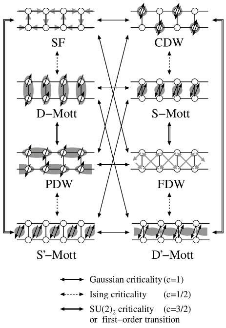
Figure 5: Schematic illustration of the phase diagram under the global SU(2) symmetry. The phase transitions indicated by the solid (dashed) arrows are the $c=1$ ($c=1/2$) criticality. The phase transitions indicated by the double arrows are either the $c=3/2$ SU(2)₂ criticality or first order; see discussion in Sec. IVC3 and Fig. 10. The diagonal solid arrows denote the Gaussian transitions in the $\phi_{\rho+}$ mode.

IV.3.2 Gaussian criticality in the charge degrees of freedom

First we discuss the Gaussian criticality when all the modes except the relative charge mode ($\rho-$) become massive at some higher energy scale. This situation is relevant for the horizontal transitions in Fig. 5: SF–CDW, D-Mott–S-Mott, PDW–FDW, and S’-Mott–D’-Mott transitions. We take the D-Mott–S-Mott phase transition as an example. Without loss of generality we may assume that the phase variables are locked at $\langle\phi_{\rho+}\rangle=\langle\phi_{\sigma+}\rangle=\langle\phi_{\sigma-}\rangle=0$ mod $\pi$. Below the energy scale at which the three fields are locked, we can replace the cosine terms in the Hamiltonian Eq. (123) by their average: $\cos 2\phi_{\rho+}\to c_{\rho+}\equiv\langle\cos 2\phi_{\rho+}\rangle$, $\cos 2\phi_{\sigma+}\to c_{\sigma+}\equiv\langle\cos 2\phi_{\sigma+}\rangle$, and $\cos 2\phi_{\sigma-}\to c_{\sigma-}\equiv\langle\cos 2\phi_{\sigma-}\rangle$, where $c_{\rho+}$, $c_{\sigma+}$, and $c_{\sigma-}$ are nonuniversal positive constants that depend on bare interactions. We then have the effective theory

$$\mathcal{H}_{\rho-}\!\! = \!\!\frac{v_{F}}{\pi}\left[(\partial_{x}\phi^{+}_{\rho-})^{2}+(\partial_{x}\phi^{-}_{\rho-})^{2}\right]$$ (134)

$$\!{}+\frac{g_{\rho-}}{2\pi^{2}}\left(\partial_{x}\phi_{\rho-}^{+}\right)\left(\partial_{x}\phi_{\rho-}^{-}\right)$$

$$\!{}+\frac{g_{\overline{c-}}}{2\pi^{2}a^{2}}\,\cos 2\theta_{\rho-},$$

where the coupling constant $g_{\overline{c-}}$ is given by

$$g_{\overline{c-}}=c_{\rho+}\,g_{c+,\overline{c-}}+c_{\sigma+}\,g_{\overline{c-},s+}+c_{\sigma-}\,g_{\overline{c-},s-}.$$ (135)

Since the canonical dimension of $\cos 2\theta_{\rho-}$ is $1$, the $g_{\overline{c-}}$ term is a relevant perturbation and hence the system always becomes massive except when $g_{\overline{c-}}=0$. If $g_{\overline{c-}}>0$, then the phase field is locked as $\langle\theta_{\rho-}\rangle=\pi/2$ mod $\pi$, which corresponds to the S-Mott phase. When $g_{\overline{c-}}<0$, the phase field is locked as $\langle\theta_{\rho-}\rangle=0$ mod $\pi$, and the ground state in this case turns out to be the D-Mott state. The Gaussian criticality with the central charge $c=1$ is realized at $g_{\overline{c-}}=0$. In terms of the original Hubbard interactions the coupling constant $g_{\overline{c-}}$ is given by

$$\frac{g_{\overline{c-}}}{a}=-C\left(U-V_{\perp}+\frac{3}{4}J_{\perp}+t_{\mathrm{pair}}\right)+C^{\prime}(V_{\parallel}-V^{\prime}),$$ (136)

where $C\equiv c_{\rho+}+c_{\sigma+}+c_{\sigma-}$ and $C^{\prime}\equiv 2c_{\rho+}+2c_{\sigma+}-c_{\sigma-}$ are nonuniversal positive constants. Thus, the D-Mott (S-Mott) state appears when $U-V_{\perp}+3J_{\perp}/4+t_{\mathrm{pair}}-C^{\prime}(V_{\parallel}-V^{\prime})/C>0$ ($<0$), and the Gaussian criticality shows up at

$$U-V_{\perp}+\frac{3}{4}J_{\perp}+t_{\mathrm{pair}}-\frac{C^{\prime}}{C}(V_{\parallel}-V^{\prime})=0,$$ (137)

which is the same as the phase boundary obtained from the strong-coupling analysis, Eq. (73), for $V_{\parallel}=V^{\prime}=0$.

The SF–CDW phase transition can be analyzed in a similar way. We consider a situation where the phase variable $\theta_{\sigma-}$, instead of $\phi_{\sigma-}$, is locked at $\langle\theta_{\sigma-}\rangle=0$ mod $\pi$. In this case we can replace the cosine factor in the Hamiltonian as $\cos 2\theta_{\sigma-}\to c_{\overline{\sigma-}}\equiv\langle\cos 2\theta_{\sigma-}\rangle>0$. The effective theory is given by Eq. (134) with the coupling constant $g_{\overline{c-}}=c_{\rho+}\,g_{c+,\overline{c-}}+c_{\sigma+}\,g_{\overline{c-},s+}+c_{\overline{\sigma-}}\,g_{\overline{c-},\overline{s-}}$. The SF (CDW) state is realized for $g_{\overline{c-}}<0$ $(>0)$, where the phase $\theta_{\rho-}$ is locked at $0$ ($\pi/2$) mod $\pi$. In terms of the original Hubbard interactions, the coupling constant $g_{\overline{c-}}$ is given by Eq. (136) with $C=c_{\rho+}+c_{\sigma+}>0$ and $C^{\prime}=2c_{\rho+}+2c_{\sigma+}+3c_{\overline{\sigma-}}$. We thus conclude that the SF (CDW) state appears for $U-V_{\perp}+\frac{3}{4}J_{\perp}+t_{\mathrm{pair}}-C^{\prime}(V_{\parallel}-V^{\prime})/C>0$ ($<0$), and the condition for the Gaussian criticality is given by Eq. (137).

The other transitions of the $c=1$ Gaussian criticality can also be analyzed in the same manner. We note that in addition to the Gaussian criticality in the $\rho-$ mode discussed above, there is another Gaussian criticality in the $\rho+$ mode that govern the SF–FDW, CDW–PDW, D-Mott–D’-Mott, and S-Mott–S’-Mott transitions.

IV.3.3 Z₂ $\times$ O(3) symmetry in the spin degrees of freedom and the Ising and SU(2)₂ criticality

Here we focus on the case where the masses of the two charge modes ($\rho\pm$) are larger than those of the spin modes ($\sigma\pm$). Below the mass scale of the charge modes we may regard that the $\phi_{\rho+}$ and $\theta_{\rho-}$ fields are locked by cosine potentials. The effective low-energy theory is obtained from Eq. (123) by replacing $\cos 2\phi_{\rho_{+}}$ and $\cos 2\theta_{\rho-}$ by their average values $c_{\rho+}\equiv\langle\cos 2\phi_{\rho+}\rangle$ and $c_{\overline{\rho-}}\equiv\langle\cos 2\theta_{\rho-}\rangle$:

$${\cal H}_{\sigma}\! = \!\frac{v_{F}}{\pi}\left[\left(\partial\phi_{\sigma+}^{+}\right)^{2}+\left(\partial\phi_{\sigma+}^{-}\right)^{2}+\left(\partial\phi_{\sigma-}^{+}\right)^{2}+\left(\partial\phi_{\sigma-}^{-}\right)^{2}\right]$$ (138)

$${}+\frac{g_{\sigma+}}{2\pi^{2}}\left(\partial\phi_{\sigma+}^{+}\right)\left(\partial\phi_{\sigma+}^{-}\right)+\frac{g_{s+}}{2\pi^{2}a^{2}}\,\cos 2\phi_{\sigma+}$$

$${}+\frac{g_{\sigma-}}{2\pi^{2}}\left(\partial\phi_{\sigma-}^{+}\right)\left(\partial\phi_{\sigma-}^{-}\right)$$

$${}+\frac{g_{s-}}{2\pi^{2}a^{2}}\,\cos 2\phi_{\sigma-}+\frac{g_{\overline{s-}}}{2\pi^{2}a^{2}}\,\cos 2\theta_{\sigma-}$$

$${}+\frac{g_{s+,s-}}{2\pi^{2}a^{2}}\,\cos 2\phi_{\sigma+}\,\cos 2\phi_{\sigma-}$$

$${}+\frac{g_{s+,\overline{s-}}}{2\pi^{2}a^{2}}\,\cos 2\phi_{\sigma+}\,\cos 2\theta_{\sigma-},$$

where the coupling constants $g_{s+}$, $g_{s-}$, and $g_{\overline{s-}}$ are given by

$$g_{s+} \equiv c_{\rho+}\,g_{c+,s+}+c_{\overline{\rho-}}\,g_{\overline{c-},s+},$$ (139a)

$$g_{s-} \equiv c_{\rho+}\,g_{c+,s-}+c_{\overline{\rho-}}\,g_{\overline{c-},s-},$$ (139b)

$$g_{\overline{s-}} \equiv c_{\rho+}\,g_{c+,\overline{s-}}+c_{\overline{\rho-}}\,g_{\overline{c-},\overline{s-}}.$$ (139c)

The coupling constants in Eq. (138) are not completely free parameters, since the system has the spin-rotational SU(2) symmetry. From Eqs. (127) and (139), the constraints on the coupling constants read

$$g_{s+}-g_{s-}-g_{\overline{s-}}=0,$$ (140a)

$$g_{s+,s-}=-\frac{1}{2}(g_{\sigma+}+g_{\sigma-}),$$ (140b)

$$g_{s+,\overline{s-}}=-\frac{1}{2}(g_{\sigma+}-g_{\sigma-}).$$ (140c)

To appreciate the SU(2) symmetry in the effective theory (138), we fermionize it by introducing spinless fermion fields $\psi_{p,r}$ ($p=\pm$ and $r=\pm$):

$$\psi_{\pm,r}(x)=\frac{\eta_{r}}{\sqrt{2\pi a}}\,\exp\left[\pm i\,2\phi_{\sigma r}^{\pm}(x)\right],$$ (141)

where the index $r=+(-)$ refers to the total (relative) degrees of freedom of spin mode, and $\{\eta_{r},\eta_{r^{\prime}}\}=2\delta_{r,r^{\prime}}$. The density operators are given by $:\!\psi_{p,\pm}^{\dagger}\,\psi_{p,\pm}\!:\,=\partial_{x}\phi_{\sigma\pm}^{p}/\pi$. We then introduce the Majorana fermions $\xi^{n}$ ($n=1\sim 4$) by

$$\psi_{p,+}=\frac{1}{\sqrt{2}}\left(\xi_{p}^{1}+i\xi_{p}^{2}\right),\hskip 5.69046pt\psi_{p,-}=\frac{1}{\sqrt{2}}\left(\xi_{p}^{4}+i\xi_{p}^{3}\right).$$ (142)

These fields satisfy the anticommutation relations $\{\xi_{p}^{n}(x),\xi_{p^{\prime}}^{n^{\prime}}(x^{\prime})\}=\delta(x-x^{\prime})\,\delta_{p,p^{\prime}}\,\delta_{n,n^{\prime}}$. With the help of the SU(2) constraints (140), we rewrite the effective Hamiltonian in terms of the Majorana fermions:

$$\mathcal{H}_{\sigma}\!\! = \!\!{}-i\frac{v_{F}}{2}\left(\bm{\xi}_{+}\cdot\partial_{x}\bm{\xi}_{+}-\bm{\xi}_{-}\cdot\partial_{x}\bm{\xi}_{-}\right)-im_{t}\,\bm{\xi}_{+}\cdot\bm{\xi}_{-}$$ (143)

$${}-i\frac{v_{F}}{2}\left(\xi_{+}^{4}\,\partial_{x}\xi_{+}^{4}-\xi_{-}^{4}\,\partial_{x}\xi_{-}^{4}\right)-im_{s}\,\xi_{+}^{4}\,\xi_{-}^{4}$$

$${}+\frac{g_{\sigma+}}{4}\,\left(\bm{\xi}_{+}\cdot\bm{\xi}_{-}\right)^{2}+\frac{g_{\sigma-}}{2}\left(\bm{\xi}_{+}\cdot\bm{\xi}_{-}\right)\,\xi_{+}^{4}\,\xi_{-}^{4},\qquad$$

where we have introduced $\mbox{\boldmath$\xi$}_{p}=(\xi_{p}^{1},\xi_{p}^{2},\xi_{p}^{3})$ and

$$m_{t}\equiv-\frac{g_{s+}}{2\pi a},\qquad m_{s}\equiv-\frac{g_{s-}-g_{\overline{s-}}}{2\pi a}.$$ (144)

Thus the effective theory for the spin sector becomes O(3)$\times$Z₂ symmetric, i.e., the four Majorana fermions are grouped into a singlet $\xi^{4}$ with mass $m_{s}$ and a triplet $\bm{\xi}$ with mass $m_{t}$. We note that the O(3)$\times$Z₂ symmetry also appears in the low-energy effective theory of the isotropic Heisenberg ladder.Shelton ; Nersesyan1997 It is known that, when $m_{s},m_{t}\neq 0$, the quartic marginal terms lead to mass renormalization, $m_{s}\to\widetilde{m}_{s}$ and $m_{t}\to\widetilde{m}_{t}$, whereShelton ; Gogolin_book

$$\widetilde{m}_{t}\!\! = \!\!m_{t}+\frac{g_{\sigma+}}{2\pi v_{F}}m_{t}\ln\frac{\Lambda}{|m_{t}|}+\frac{g_{\sigma-}}{4\pi v_{F}}m_{s}\ln\frac{\Lambda}{|m_{s}|},\qquad$$ (145)

$$\widetilde{m}_{s}\!\! = \!\!m_{s}+\frac{3g_{\sigma-}}{4\pi v_{F}}m_{t}\ln\frac{\Lambda}{|m_{t}|}.$$ (146)

Here $\Lambda$ is a high-energy cutoff. The effective theory then reduces to

$$\mathcal{H}_{\sigma} \!\!=\!\! {}-i\frac{v_{F}}{2}\left(\bm{\xi}_{+}\cdot\partial_{x}\bm{\xi}_{+}-\bm{\xi}_{-}\cdot\partial_{x}\bm{\xi}_{-}\right)-i\widetilde{m}_{t}\,\bm{\xi}_{+}\cdot\bm{\xi}_{-}$$ (147)

$${}-i\frac{v_{F}}{2}\left(\xi_{+}^{4}\,\partial_{x}\xi_{+}^{4}-\xi_{-}^{4}\,\partial_{x}\xi_{-}^{4}\right)-i\widetilde{m}_{s}\,\xi_{+}^{4}\,\xi_{-}^{4}.$$

It immediately follows from Eq. (147) that the Ising criticality with $c=1/2$ emerges as $\widetilde{m}_{s}\to 0$. On the other hand, the critical properties for the O(3) invariant sector ($\widetilde{m}_{t}\to 0$) is known to be described by the SU(2)₂ Wess-Zumino-Novikov-Witten model with the central charge $c=3/2$. Gogolin_book ; Tsvelik1990

Let us examine the critical behavior in more detail using the scaling equations for the coupling constants appearing in the effective Hamiltonian (143):

$$\frac{dG_{t}}{dl}\!\! = \!\!G_{t}+G_{t}G_{\sigma+}+\frac{1}{2}G_{s}G_{\sigma-},$$ (148a)

$$\frac{dG_{s}}{dl}\!\! = \!\!G_{s}+\frac{3}{2}G_{t}G_{\sigma-},$$ (148b)

$$\frac{dG_{\sigma+}}{dl}\!\! = \!\!\frac{1}{2}G_{\sigma+}^{2}+\frac{1}{2}G_{\sigma-}^{2}+2G_{t}^{2},$$ (148c)

$$\frac{dG_{\sigma-}}{dl}\!\! = \!\!G_{\sigma+}G_{\sigma-}+2G_{t}G_{s},$$ (148d)

where $dl=da/a$, $G_{t}=-g_{s+}/2\pi v_{F}$, $G_{s}=-(g_{s-}-g_{\overline{s-}})/2\pi v_{F}$, and $G_{\sigma\pm}=g_{\sigma\pm}/2\pi v_{F}$. The coupling $G_{s}$ and $G_{t}$ are relevant, while $G_{\sigma\pm}$ are marginal. Within the one-loop RG we find 4 stable fixed points, $(G_{t}^{*},G_{s}^{*},G_{\sigma+}^{*},G_{\sigma-}^{*})=(\pm\infty,\pm\infty,\infty,\infty)$ and $(\pm\infty,\mp\infty,\infty,-\infty)$, which correspond to the 8 phases listed in Fig. 5 and Table 2. The Ising criticality is governed by the unstable fixed point $(G_{t}^{*},G_{s}^{*},G_{\sigma+}^{*},G_{\sigma-}^{*})=(\pm\infty,0,\infty,0)$, where the Majorana fermion $\xi^{4}$ is massless. The unstable fixed point $(G_{t}^{*},G_{s}^{*},G_{\sigma+}^{*},G_{\sigma-}^{*})=(0,\pm\infty,0,0)$ corresponds to the SU(2)₂ criticality since the triplet $\bm{\xi}$ becomes massless. Finally, we find another kind of unstable fixed points $(G_{t}^{*},G_{s}^{*},G_{\sigma+}^{*},G_{\sigma-}^{*})=(0,\pm\infty,\infty,0)$, where all the modes are massive. To understand the nature of these unstable fixed points, let us assume $(g_{s+},g_{\overline{s-}}-g_{s-},g_{\sigma+},g_{\sigma-})=(0,2\lambda_{1},2\lambda_{2},0)$, where $\lambda_{1,2}$ are constants ($\lambda_{1}\neq 0$, $\lambda_{2}>0$). This, together with the SU(2) constraint (140), leads to $g_{\overline{s-}}=-g_{s-}=\lambda_{1}$ and $g_{s+,\overline{s-}}=g_{s+,s-}=-\lambda_{2}<0$. In this case the cosine terms in $\mathcal{H}_{\sigma}$ (138) become

$${}-\frac{\lambda_{1}}{2\pi^{2}a^{2}}(\cos 2\phi_{\sigma-}-\cos 2\theta_{\sigma-})$$

$${}-\frac{\lambda_{2}}{2\pi^{2}a^{2}}\cos 2\phi_{\sigma+}(\cos 2\phi_{\sigma-}+\cos 2\theta_{\sigma-}).\qquad$$ (149)

Suppose that $\lambda_{1}>0$ and $\langle\phi_{\rho+}\rangle=\langle\theta_{\rho-}\rangle=0$. We then find that the potential (149) has degenerate minima at, e.g., $(\langle\phi_{\sigma+}\rangle,\langle\phi_{\sigma-}\rangle,\langle\theta_{\sigma-}\rangle)=(0,0,*)$ and $(\frac{\pi}{2},*,\frac{\pi}{2})$, where $*$ means that the phase field is not locked. Since these minima correspond to the D-Mott and PDW phases, the unstable fixed point describes a first-order transition between the D-Mott and PDW phases, respectively. Hence we conclude that the unstable fixed points $(G_{t}^{*},G_{s}^{*},G_{\sigma+}^{*},G_{\sigma-}^{*})=(0,\pm\infty,\infty,0)$ correspond to a first-order phase transition. The phase transition at which the renormalized triplet mass $G_{t}^{*}$ vanishes can be either SU(2)₂ criticality or first-order transition, depending on the sign of $G_{\sigma+}$ Shankar . The condition for the SU(2)₂ criticality is $G_{t}=0$ and $G_{\sigma+}<0$ below the energy scale where $G_{s}$ becomes of order 1. On the other hand, the first-order transition is realized if $G_{t}=0$ and $G_{\sigma+}>0$.

Table 2: Signs of the fixed-point coupling constants and the masses ($m_{g}$, $\widetilde{m}_{s}$, $\widetilde{m}_{t}$) in various phases.

Phase	$(g_{\overline{c-}}^{*},g_{s+}^{*},g_{s-}^{*},g_{\overline{s-}}^{*},g_{\sigma+}^{*},g_{\sigma-}^{*})$	$m_{g}$	$\widetilde{m}_{s}$	$\widetilde{m}_{t}$
CDW	$(+,-,0,-,+,-)$	$+$	$-$	$+$
SF	$(-,-,0,-,+,-)$	$-$	$-$	$+$
PDW	$(-,+,0,+,+,-)$	$-$	$+$	$-$
FDW	$(+,+,0,+,+,-)$	$+$	$+$	$-$
S-Mott	$(+,-,-,0,+,+)$	$+$	$+$	$+$
D-Mott	$(-,-,-,0,+,+)$	$-$	$+$	$+$
S’-Mott	$(-,+,+,0,+,+)$	$-$	$-$	$-$
D’-Mott	$(+,+,+,0,+,+)$	$+$	$-$	$-$

The phase fields are locked at some multiples of $\pi/2$ depending on signs of the relevant coupling constants at a fixed point, $(g_{\overline{c-}}^{*},g_{s+}^{*},g_{s-}^{*},g_{\overline{s-}}^{*})$, of the cosine potentials in Eqs. (134) and (138). Comparing the configuration of the locked phases and those listed in Table 1, we can find out to which phase the ground state belongs for given combination of the renormalized coupling constants, $(g_{\overline{c-}}^{*},g_{s+}^{*},g_{s-}^{*},g_{\overline{s-}}^{*})$. Table 2 summarizes for each phase the signs of these renormalized coupling constants including $g_{\sigma\pm}^{*}$, which is positive (negative) when $\phi_{\sigma\pm}$ ($\theta_{\sigma\pm}$) is locked. When writing Table 2, we have used the fact (a) that either one of $g_{s-}^{*}$ and $g_{\overline{s-}}^{*}$ must vanish except at the Ising criticality because $\phi_{\sigma-}$ and $\theta_{\sigma-}$ are conjugate fields, and (b) that Eq. (140a) constraints possible combinations of signs of $g_{s+}$, $g_{s-}$, and $g_{\overline{s-}}$.

The coupling constants listed in Table 2 also determine the signs of masses $m_{g}(=g_{\overline{c-}}/2\pi a)$, $\widetilde{m}_{s}$, and $\widetilde{m}_{t}$ through Eqs. (144), (145), and (146). The Gaussian ($c=1$), Ising ($c=1/2$), and SU(2)₂ ($c=3/2$) criticalities are realized when $m_{g}=0$, $\widetilde{m}_{s}=0$, and $\widetilde{m}_{t}=0$, respectively. From Table 2 we can therefore figure out which criticality can occur at each phase transition where the relevant mass changes sign. The universality class of the phase transitions is also summarized in Fig. 5. We find from Table 2 that the CDW–S-Mott and SF–D-Mott phase transitions are indeed in the Ising universality class and the D-Mott–S-Mott phase transition is in the Gaussian universality class, in agreement with the strong-coupling approach in Sec. III.

Let us discuss implications of the above general qualitative analysis to the phase diagram of the extended Hubbard ladder. From Eqs. (139) and (144) we write the bare masses in terms of the coupling constants in the model:

$$m_{s}\!\! = \!\!\frac{1}{2\pi}\biggl{[}2c_{\rho+}(U-t_{\mathrm{pair}}+V^{\prime})$$

$$\quad{}+c_{\overline{\rho-}}\left(U-V_{\perp}+\frac{3}{4}J_{\perp}+t_{\mathrm{pair}}-4V^{\prime}\right)\biggr{]},$$

$$m_{t}\!\! = \!\!\frac{1}{2\pi}\left[2c_{\rho+}\left(V_{\perp}+\frac{1}{4}J_{\perp}-\frac{3}{2}V^{\prime}\right)\right.$$

$$\quad\left.{}+c_{\overline{\rho-}}\left(U-V_{\perp}+\frac{3}{4}J_{\perp}+t_{\mathrm{pair}}+2V^{\prime}\right)\right].$$

To simplify the discussion, we assume here that $V_{\parallel}=V^{\prime}=t_{\mathrm{pair}}=0$ and that $\phi_{\rho+}$ is locked at $\langle\phi_{\rho+}\rangle=0$ (mod $\pi$), i.e., $c_{\rho+}>0$. If $U-V_{\perp}+3J_{\perp}/4>0$ ($<0$), the phase $\theta_{\rho-}$ is locked at $0$ ($\pi/2$) [see Eq. (136)] and $c_{\overline{\rho-}}=\langle\cos 2\theta_{\rho-}\rangle>0$ $(<0)$. Thus, the product $c_{\overline{\rho-}}(U-V_{\perp}+3J_{\perp}/4)$ is positive for both positive and negative $U-V_{\perp}+3J_{\perp}/4$, and hence the bare masses $m_{s}$ and $m_{t}$ are also positive. We argue, however, that the Ising criticality is possible due to the mass renormalization effect. The renormalized mass $\widetilde{m}_{s}$ can become negative since the coupling constant $g_{\sigma-}$ of the correction term in Eq. (146) is given by $g_{\sigma-}=2a(-V_{\perp}+J_{\perp}/4)$. We expect that sufficiently large $V_{\perp}$ can drive the system toward the Ising criticality in the $\xi^{4}$ mode, even when $t_{\mathrm{pair}}=0$.

In addition to the Ising criticality at large $V_{\perp}$, the Gaussian criticality in the $\theta_{\rho-}$ mode should appear at $V_{\perp}=U+3J_{\perp}/4$. Let us find out which phase is realized near the Gaussian critical line. When $U-V_{\perp}+3J_{\perp}/4=0$, the coupling $g_{\sigma-}$ equals $-2U-J_{\perp}$ and the renormalized Ising mass becomes

$$\frac{\widetilde{m}_{s}}{c_{\rho+}U}=1-A\frac{U}{\Lambda}\left(1+\frac{3J_{\perp}}{U}+\frac{2J_{\perp}^{2}}{U^{2}}\right)\ln\left(\frac{\Lambda}{U+J_{\perp}}\right),$$ (152)

where $A$ is a positive constant of order 1. For small $J_{\perp}/U$ this renormalized Ising mass should be positive, and we conclude that the D-Mott and the S-Mott phases are separated by the Gaussian critical line (Note that $\widetilde{m}_{t}>0$). As we increase $J_{\perp}/U$ (or $V_{\perp}/U$) along the Gaussian critical line, the negative correction ($\propto g_{\sigma-}$) in the mass renormalization increases and eventually $\widetilde{m}_{s}$ can change sign. Across this Ising transition the D-Mott and S-Mott phases turn into the SF and CDW phases, respectively. This implies that a pair of phases surrounding the Gaussian critical line changes from (D-Mott,S-Mott) to (SF,CDW) at a tetracritical point as $J_{\perp}/U$ increases. This qualitative analysis will be supported in the next subsection by a more quantitative renormalization group analysis.

Now we briefly discuss the effect of the pair hopping term $t_{\mathrm{pair}}$ and next-nearest-neighbor repulsion $V^{\prime}$. When $V^{\prime}=0$, the Gaussian transition takes place at $U-V_{\perp}+3J_{\perp}/4+t_{\mathrm{pair}}=0$ [see Eq. (137)]. Thus for large $t_{\mathrm{pair}}$, we can have a situation where $m_{s}<0$ and $m_{t}>0$ with $U-V_{\perp}+3J_{\perp}/4+t_{\mathrm{pair}}\simeq 0$ [see Eqs. (LABEL:eq:ms_bare) and (LABEL:eq:mt_bare)], i.e., $t_{\mathrm{pair}}$ can stabilize the SF state near the Gaussian critical line. In the case $t_{\mathrm{pair}}=0$, on the other hand, we expect that sufficiently large $V^{\prime}$ can lead to a phase with $m_{s}>0$ and $m_{t}<0$ i.e., the PDW state, if $c_{\rho+}\gg c_{\overline{\rho-}}>0$.

Finally, we discuss implications of our schematic phase diagram (Fig. 5) to the phase diagram of isotropic spin-$\frac{1}{2}$ ladder systems, which have been studied intensively in connection with the so-called Haldane’s conjecture Haldane about the existence of a finite energy gap in the integer-spin Heisenberg chain. By using the abelian bosonization method, it has been shown that four kinds of gapped phases can appear in spin ladder systems with various types of exchange interactions. Kim ; Gogolin_book The possible gapped phases are (1) the rung singlet state, which is known to be realized in the isotropic Heisenberg ladder with nearest-neighbor antiferromagnetic exchange couplings, (2) the Affleck-Kennedy-Lieb-Tasaki(AKLT)-like spin liquid state, in which short-range valence bonds couple spins on neighboring rungs, AKLT (3) the dimerized state along chain with $\pi$ relative phase, and (4) the dimerized state along chain with zero relative phase. Both the rung single state and the AKLT-like state are Haldane-type spin liquids with unique ground state and no broken local symmetries. In the dimerized states which are known to be realized when a sufficiently strong four-spin interaction is included, Nersesyan1997 ; Gogolin_book there is spontaneous breaking of the translation ($Z_{2}$) symmetry and the ground state is two-fold degenerate. In the limit of large $U$ the extended Hubbard ladder we analyze in this paper should reduce to a system with only the spin degrees of freedom. This situation corresponds to $g_{\overline{c-}}<0$ [see Eq. (136)], i.e., $m_{g}<0$, with $|m_{g}|\gg|\tilde{m}_{s}|,|\tilde{m}_{t}|$. Under this condition, we still have four phases: the SF, D-Mott, PDW, and S’-Mott phases. From Table 2 (see also Refs. Nersesyan1997, ; Gogolin_book, ; Kim, ), we can find correspondence between the phases in spin ladders and the phases which we have obtained in the extended Hubbard ladders: The rung-singlet and AKLT-like Haldane states correspond to the D-Mott and S’-Mott states, respectively, and the PDW (SF) state corresponds to the dimerized state along chain with $\pi$ (0) relative phase. We note that physical pictures of phases in the extended Hubbard ladder are consistent with those in spin ladder; for example, the D-Mott state is nothing bug the rung singlet state, as seen in the strong-coupling approach (see Sec. III). The AKLT-like Haldane state, which is known to be realized either with plaquette diagonal exchange coupling or with ferromagnetic rung exchange,Kim would be smoothly connected to the S’-Mott state, in which the ground-state wave function consists of singlets formed between diagonal sites of plaquettes [see Eq. (132)] and, moreover, has the same topological numbers as the AKLT-like Haldane state.Kim The PDW state is nothing but the dimerized state with interchain phase $\pi$ as seen in Fig. 5, which is not a Haldane-type spin liquid since the PDW state spontaneously breaks translation symmetry and is two-fold degenerate. In order to discuss phase transitions in spin ladder systems, two kinds of string order parameters have been introduced which characterize hidden orders with different topological numbers, i.e., the parity of the number of dimers crossing a line perpendicular to the two chains. Nishiyama ; Kim These string order parameters are different from $\mu_{j}$ (Eq. (129)), since $\mu_{j}$ is associated with $\exp(i\phi_{\sigma-})$ in the bosonized form while the string order parameters introduced in Refs. Kim, and Nishiyama, are associated with the $\phi_{\sigma+}$ field in our notation. Since the phase transition associated with the $\phi_{\sigma+}$ field is related to $\widetilde{m}_{t}\to 0$, we expect that the string order parameters introduced in Refs. Kim, and Nishiyama, characterize the SU(2)₂ criticality or the first-order phase transition (double arrows in Fig. 5). In our schematic phase diagram (5) the phase transition from the rung singlet state to the AKLT Haldane state can take place (which is actually the case in the spin-$\frac{1}{2}$ ladder systemsKim ; Hakobyan ), if the SU(2)₂ and the Ising criticalities appear simultaneously. This implies that the central charge for the continuous transition between the rung singlet and the AKLT states is given by $\frac{3}{2}+\frac{1}{2}=2$. This transition becomes first order when the marginal interaction in the triplet Majorana fermion sector is marginally relevant.

IV.4 Renormalization group analysis

In this subsection, we study the ground-state phase diagram of the extended Hubbard ladder model using perturbative RG analysis of the 13 coupling constants appearing in Eq. (123). These coupling constants are, however, not independent because of the 4 constraints coming from the SU(2) symmetry, Eq. (127). Accordingly, we have 9 independent RG equations that describe how the coupling constants scale when we change the lattice constant $a\to ae^{dl}$. The 9 independent variables we choose to work with are: $G_{\rho+}\equiv g_{\rho+}/2\pi v_{F}$, $G_{\rho-}\equiv g_{\rho-}/2\pi v_{F}$, $G_{\sigma+}\equiv g_{\sigma+}/2\pi v_{F}$, $G_{\sigma-}\equiv g_{\sigma-}/2\pi v_{F}$, $G_{\alpha}\equiv(g_{c+,s-}-g_{c+,\overline{s-}})/2\pi v_{F}$, $G_{\beta}\equiv(g_{\overline{c-},s-}-g_{\overline{c-},\overline{s-}})/2\pi v_{F}$, $G_{A}\equiv g_{c+,\overline{c-}}/2\pi v_{F}$, $G_{B}\equiv g_{c+,s+}/2\pi v_{F}$, and $G_{C}\equiv g_{\overline{c-},s+}/2\pi v_{F}$. After some algebra we obtain the RG equations:

$$\frac{d}{dl}G_{\rho+}\!\! = \!\!+G_{A}^{2}+\frac{3}{2}G_{B}^{2}+\frac{1}{2}G_{\alpha}^{2},$$ (153)

$$\frac{d}{dl}G_{\rho-}\!\! = \!\!-G_{A}^{2}-\frac{3}{2}G_{C}^{2}-\frac{1}{2}G_{\beta}^{2},$$ (154)

$$\frac{d}{dl}G_{\sigma+}\!\! = \!\!+\frac{1}{2}G_{\sigma+}^{2}+\frac{1}{2}G_{\sigma-}^{2}+G_{B}^{2}+G_{C}^{2},$$ (155)

$$\frac{d}{dl}G_{\sigma-}\!\! = \!\!+G_{\sigma+}\,G_{\sigma-}+G_{B}\,G_{\alpha}+G_{C}\,G_{\beta},$$ (156)

$$\frac{d}{dl}G_{A}\!\! = \!\!+\frac{1}{2}G_{\rho+}\,G_{A}-\frac{1}{2}G_{\rho-}\,G_{A}$$ (157)

$$-\frac{3}{2}G_{B}\,G_{C}-\frac{1}{2}G_{\alpha}G_{\beta},$$

$$\frac{d}{dl}G_{B}\!\! = \!\!+\frac{1}{2}G_{\rho+}\,G_{B}+G_{\sigma+}\,G_{B}$$ (158)

$$-G_{A}\,G_{C}+\frac{1}{2}G_{\sigma-}\,G_{\alpha},$$

$$\frac{d}{dl}G_{C}\!\! = \!\!-\frac{1}{2}G_{\rho-}\,G_{C}+G_{\sigma+}\,G_{C}$$ (159)

$$-G_{A}\,G_{B}+\frac{1}{2}G_{\sigma-}\,G_{\beta},$$

$$\frac{d}{dl}G_{\alpha}\!\! = \!\!+\frac{1}{2}G_{\rho+}\,G_{\alpha}+\frac{3}{2}G_{B}\,G_{\sigma-}-G_{A}\,G_{\beta},$$ (160)

$$\frac{d}{dl}G_{\beta}\!\! = \!\!-\frac{1}{2}G_{\rho-}\,G_{\beta}+\frac{3}{2}G_{C}\,G_{\sigma-}-G_{A}\,G_{\alpha}.\qquad$$ (161)

These equations are equivalent to the ones reported in Ref. Lin, , in which another set of 9 independent variables are used: $b_{11}^{\rho}=(g_{\rho+}+g_{\rho-})/8$, $b_{11}^{\sigma}=-(g_{\sigma+}+g_{\sigma-})/2$, $b_{12}^{\rho}=g_{\beta}/4$, $b_{12}^{\sigma}=g_{C}$, $f_{12}^{\rho}=(g_{\rho+}-g_{\rho-})/8$, $f_{12}^{\sigma}=-(g_{\sigma+}-g_{\sigma-})$, $u_{11}^{\rho}=-g_{A}/8$, $u_{12}^{\rho}=g_{\alpha}/8$, and $u_{12}^{\sigma}=g_{B}/2$, where $g_{\nu}=2\pi v_{F}G_{\nu}$.

Figure 6: Weak-coupling phase diagram of $H_{t_{\parallel}}+H_{t_{\perp}}+H_{\mathrm{int}}$ at $t_{\perp}=t_{\parallel}=t$ and $J_{\perp}=0$ obtained from the 1-loop RG equations. There is a massless mode (C1S0) on the boundary between the D-Mott and the S-Mott states while the boundary between the S-Mott and the CDW state is C0S$\frac{1}{2}$.

Figure 7: Weak-coupling phase diagram of $H_{t_{\parallel}}+H_{t_{\perp}}+H_{\mathrm{int}}$ at $t_{\perp}=t_{\parallel}$ and $U/t=1$. This corresponds to Fig. 2. Inset shows weak-coupling phase diagram of $H_{t_{\parallel}}+H_{t_{\perp}}+H_{\mathrm{int}}+H_{\mathrm{pair}}$ at $t_{\perp}=t_{\parallel}=t$, $U/t=1$, and $t_{\mathrm{pair}}/t=0.5$. On the boundaries between the D-Mott and the S-Mott states and between the SF and the CDW states exists a massless mode C1S0. A massless mode C0S$\frac{1}{2}$ appears on the boundaries between the D-Mott and the SF states and between the S-Mott and the CDW states. The different choice of $U/t$ does not yield qualitative changes to this phase diagram.

Integrating the RG equations (153)-(161) numerically with the initial condition set by the bare coupling constants in the extended Hubbard ladder model, we find that $G_{\rho+}(l)$ grows most rapidly and becomes of order unity first. At the length scale $l=l_{\rho+}$ where $G_{\rho+}(l_{\rho+})=2$, we stop the numerical integration. Below this energy scale the $\rho+$ mode becomes massive. We can assume without losing generality that the phase $\phi_{\rho+}$ is locked at $\langle\phi_{\rho+}\rangle=0$ mod $\pi$. The effective theory at lower energy scale ($l>l_{\rho+}$) is obtained from Eq. (123) through the substitution $\cos 2\phi_{\rho+}\to 1$, $g_{c+,\overline{c-}}\to g_{\overline{c-}}$, $g_{c+,s+}\to g_{s+}$, $g_{c+,s-}\to g_{s-}$, and $g_{c+,\overline{s-}}\to g_{\overline{s-}}$. We then derive and solve the RG equations for the coupling constants in the effective theory to understand the low-energy properties of the remaining modes. The pattern of phase locking can be found from asymptotic low-energy behavior of the $g_{\overline{c-}}$, $g_{s+}$, $g_{s-}$, and $g_{\overline{s-}}$ in the numerical solution of the RG equations. The phase field $\Phi$ ($=\phi_{\sigma\pm}$ or $\theta_{\rho(\sigma)-}$) is locked at $\langle\Phi\rangle=\pi/2$ or 0, if the coupling constant $g$ ($g\in\{g_{\overline{c-}},g_{s+},g_{s-},g_{\overline{s-}}\}$) behaves as $g\to+C$ or $-C$ in the low-energy limit, respectively, where $C$ is a positive constant of order unity. Once the configuration of the locked phase fields is determined, the resulting ground state is found from Table 1. The phase diagram of the extended Hubbard ladder obtained in this way is shown in Figs. 6–10. We note that this approach reproduces the phase diagram of the SO(5) symmetric ladder obtained in earlier studies. Lin ; Fjaerestad Since the exotic phases like the SF state and the S-Mott state appear only for a negative $U$ in this model, we will not further discuss it as we concentrate on the case with positive $U$ and $V$ in this paper.

Let us first consider the simple case where $U$ and $V_{\perp}$ are the only electron-electron interactions. The phase diagram on the plane of $U/t$ and $V_{\perp}/t$ is shown in Fig.  6. In this and other phase diagrams shown below, all the modes are gapped everywhere except on the phase boundaries. With the standard notation C$n$S$m$ of representing a state having $n$ massless charge modes and $m$ massless spin modes,Balents1996 the three phases in Fig. 6 are characterized as the “C0S0” phase.Balents1996 ; Lin The phase boundary between the D-Mott state and the S-Mott state is the U(1) Gaussian critical line of the $\rho-$ mode (C1S0), which is given by $V_{\perp}=U$; see Eq. (137) with $J_{\perp}=0$. The phase boundary between the S-Mott state and the CDW state is the Ising critical line of the spin $\sigma-$ mode, which is C0S$\frac{1}{2}$. This weak-coupling phase diagram is similar to Fig. 1 obtained from the strong-coupling approach.

Next, we include the AF exchange coupling $J_{\perp}$. The phase diagram on the plane of $J_{\perp}/U$ and $V_{\perp}/U$ at $U/t=1$ is shown in Fig. 7. A different choice of $U/t$ does not lead to qualitative changes in the $J_{\perp}/U$ vs $V_{\perp}/U$ phase diagram. An interesting new feature is that the SF phase shows up between the D-Mott phase and the CDW phase. This is in agreement with the qualitative analysis of the previous subsection, where it is found that the exchange interaction $J_{\perp}$ suppresses the S-Mott phase and helps the SF phase appear. The Gaussian criticality of the $\rho-$ mode (C1S0) emerges on the almost straight phase boundary between the D-Mott phase and the S-Mott phase and between the SF phase and the CDW phase. This critical line is given by $V_{\perp}/U=1+3J_{\perp}/4U$, in accordance with Eq. (137). The phase boundary between the D-Mott phase and the SF phase and between the S-Mott phase and the CDW phase is the Ising criticality C0S$\frac{1}{2}$. A tetracritical point of C1S$\frac{1}{2}$ appears at the point where the two kinds of phase boundaries cross. The inset of Fig. 7 shows the phase diagram at $t_{\mathrm{pair}}=0.5t$. We see clearly that the pair-hopping favors the SF phase over the S-Mott phase. In the strong-coupling perturbation theory, we have introduced the pair-hopping term $H_{\mathrm{pair}}$ to stabilize the SF state. This is not necessary, however, in the weak-coupling approach, where the pair-hopping process is effectively generated from the second-order process in the rung hopping $t_{\perp}$. In fact, we can show that positive pair-hopping terms are generated in the renormalization-group procedure in the SF phase.Tsuchiizu2001

Figure 8: Weak-coupling phase diagram of $H$ for $U/t=1$, $V_{\parallel}=V_{\perp}=V$, and $t_{\mathrm{pair}}=V^{\prime}=0$. The tetracritical point with $C1S\frac{1}{2}$ is at $(J_{\perp}/t,V_{\perp}/t)\simeq(0.40,0.43)$.

Next we turn on the nearest-neighbor Coulomb repulsion in the leg direction, $V_{\parallel}$. The phase diagram for $V_{\parallel}=V_{\perp}(\equiv V)$ is shown in Fig. 8. Even though the additional $V_{\parallel}$ interaction strongly favors the CDW state, a small region of the S-Mott phase still remains in between the D-Mott phase and the CDW phase. Besides this quantitative modification the phase diagram is not changed qualitatively, and, in particular, the critical properties at the phase boundaries are the same as in Figs. 6 and 7. Using the density matrix renormalization group method, Vojta et al.Vojta1999 determined the phase boundary between the CDW state and a state with homogeneous charge density for the model we used for Fig. 8. At $U=1.5t$ they observed a transition to the CDW state around $U/V\approx 2.9$, which is not very different from the phase boundary at $J_{\perp}=0$ in Fig. 8. The transition is, however, found to be first order for $U\geq 4t$ in their numerical results, which is different from the continuous transition we found in the weak-coupling analysis. A possible source of this discrepancy might be the neglect of irrelevant operators with canonical dimension 4 that could become important for strong couplings as in the single chain case.Tsuchiizu2002

Figure 9: Weak-coupling phase diagram of $H$ on the plane of $U/t$ and $V^{\prime}/t$ for $V_{\parallel}=V_{\perp}=0$, and $J_{\perp}=t_{\mathrm{pair}}=0$. The boundary between the D-Mott state and the PDW state is C0S$\frac{3}{2}$, and the boundary between the PDW state and the S’-Mott state is C0S$\frac{1}{2}$.

Figure 10: Weak-coupling phase diagram of $H$ on the plane of $V^{\prime}/U$ and $V/U$ for $U/t=0.5$, $V_{\parallel}=V_{\perp}=V$, and $J_{\perp}=t_{\mathrm{pair}}=0$. The phase transition between the CDW and S-Mott phases and between the PDW and S’-Mott phases is in the Ising universality class (C0S$\frac{1}{2}$). The phase transition between Mott phases is a Gaussian transition (C1S0). The boundary between the D-Mott phase and the PDW phase is C0S$\frac{3}{2}$ [SU(2)₂ criticality]. The transition between the CDW phase and the D’-Mott phase shown by the thick solid line is a first-order transition.

Finally, we include next-nearest-neighbor Coulomb repulsion $V^{\prime}$, Eq. (9). Figures 9 and 10 show the $V^{\prime}$-$U$ and $V$-$V^{\prime}$ phase diagrams. In agreement with the discussion in the previous subsection, the PDW phase appears as $V^{\prime}$ is increased. At even larger $V^{\prime}$ the S’-Mott phase and the D’-Mott phase appear in Figs. 9 and 10. On the phase boundary between the D-Mott state and the PDW state appears the SU(2)₂ criticality; we have confirmed in our numerical calculation that the coupling $g_{\sigma+}$ in Eq. (143) is negative, i.e., marginally irrelevant. We have thus established that the two-particle interaction $V^{\prime}$ can drive the system to the SU(2)₂ criticality.

Figure 10 shows a rich phase diagram containing the four Mott phases and the two density-wave phases. We note that in Fig. 10 the six phase boundaries meet at $V=V^{\prime}=U$, which corresponds to C2S2. This happened because, within our approximation, all the coupling constants in Eq. (123) except $g_{\rho+}$ vanish when $U=V=V^{\prime}$, $t_{\perp}=t_{\parallel}$, and $J_{\perp}=t_{\mathrm{pair}}=0$. If $t_{\perp}\neq t_{\parallel}$, or if higher-order contributions to the $g$’s are included,Tsuchiizu2002 this special situation might not occur. In Fig. 10 the phase boundaries between the Mott phases are C1S0 (Gaussian criticality), while the CDW–S-Mott and PDW–S’-Mott phase boundaries are C0S$\frac{1}{2}$ (Ising criticality). The phase boundary between the PDW phase and the D-Mott phase is C0S$\frac{3}{2}$ [SU(2)₂ criticality] as in Fig. 9. Finally, the phase transition between the CDW phase and the D’-Mott phase is found to be first order; we have confirmed that the coupling $g_{\sigma+}$ in Eq. (143) is positive and marginally relevant. Even though Fig. 10 is obtained from the weak-coupling RG equations, we think that the phase diagram is reliable since we have confirmed that the $V/U$-$V^{\prime}/U$ phase diagram is not changed much when $U/t$ is varied.

V Conclusions

In this paper we have studied the half-filled generalized Hubbard ladder with the inter-site Coulomb repulsion and the exchange interaction by using the strong-coupling perturbation theory and the weak-coupling bosonization method. In the strong-coupling approach the SF state is described as an AF ordered state of the Ising model where pseudo-spins represent the currents flowing along the rungs. We have shown that the SF state can appear next to the CDW state and the D-Mott state in the phase diagram and that the quantum phase transition between the SF state and the D-Mott state is in the Ising universality class. We have also established the Ising transition between the S-Mott and the CDW phases and the Gaussian transition between the D-Mott and the S-Mott phases. In the weak-coupling approach we have shown that in general the model can accommodate total of eight insulating phases at half-filling, four density-wave phases and four Mott phases (Fig. 5). The universality class of the phase transitions among these phases is determined. In particular, we have shown that the SU(2)₂ criticality with the central charge $c=3/2$ is induced by the next-nearest-neighbor Coulomb repulsion $V^{\prime}$, which drives the system from the D-Mott phase to the PDW phase (Figs. 9 and 10). When $V^{\prime}$ is further increased, the S’-Mott phase and the D’-Mott phase, which correspond to the quantum disordered states of the PDW phase and the FDW phase, show up (Fig. 9).

When this manuscript was almost completed, we became aware of the work by Wu et al.,Fradkin2002 where the 8 insulating phases in Sec. IV are obtained independently.

References

• (1) For a review, E. Dagotto and T.M. Rice, Science 271, 618 (1996), and references therein.
• (2) M. Azuma, Z. Hiroi, M. Takano, K. Ishida, and Y. Kitaoka, Phys. Rev. Lett. 73, 3463 (1994).
• (3) K. Ishida, Y. Kitaoka, K. Asayama, M. Azuma, Z. Hiroi, and M. Takano, J. Phys. Soc. Jpn. 63, 3222 (1994).
• (4) K. Kojima, A. Keren, G.M. Luke, B. Nachumi, W.D. Wu, Y.J. Uemura, M. Azuma, and M. Takano, Phys. Rev. Lett. 74, 2812 (1995).
• (5) M. Uehara, T. Nagata, J. Akimitsu, H. Takahashi, N. Môri, and K. Kinoshita, J. Phys. Soc. Jpn.  65, 2764 (1996).
• (6) G. Blumberg, P. Littlewood, A. Gozar, B.S. Dennis, N. Motoyama, H. Eisaki, and S. Uchida, Science 297, 584 (2002), and references therein.
• (7) B. Gorshunov, P. Haas, T. Rõõm, M. Dressel, T. Vuletic, B. Hamzic, S. Tomic, J. Akimitsu, and T. Nagata, cond-mat/0201413.
• (8) E. Dagotto, J. Riera, and D. Scalapino, Phys. Rev. B 45, 5744 (1992)
• (9) A.M. Finkel’stein and A.I. Larkin, Phys. Rev. B 47, 10461 (1993).
• (10) T.M. Rice, S. Gopalan, and M. Sigrist, Europhys. Lett. 23, 445 (1993); S. Gopalan, T.M. Rice, and M. Sigrist, Phys. Rev. B 49, 8901 (1994).
• (11) M. Fabrizio, Phys. Rev. B 48, 15838 (1993).
• (12) M. Sigrist, T.M. Rice, and F.C. Zhang, Phys. Rev. B 49, 12058 (1994).
• (13) H. Tsunetsugu, M. Troyer, and T.M. Rice, Phys. Rev. B 49, 16078 (1994); M. Troyer, H. Tsunetsugu, and T.M. Rice, ibid53, 251 (1996).
• (14) D.V. Khveshchenko and T.M. Rice, Phys. Rev. B 50, 252 (1994); D.V. Khveshchenko, ibid50, 380 (1994).
• (15) R.M. Noack, S.R. White, and D.J. Scalapino, Phys. Rev. Lett. 73, 882 (1994); Physica C 270, 281 (1996).
• (16) N. Nagaosa, Solid State Commun. 94, 495 (1995).
• (17) H.J. Schulz, Phys. Rev. B 53, 2959 (1996); in Correlated Fermions and Transport in Mesoscopic Systems, edited by T. Martin, G. Montambaux, and T. Trân Thanh Vân (Editions Frontières, Gif-sur-Yvette, France, 1996), p. 81.
• (18) L. Balents and M.P.A. Fisher, Phys. Rev. B 53, 12133 (1996).
• (19) K. Sano, J. Phys. Soc. Jpn. 65, 1146 (1996).
• (20) E. Orignac and T. Giamarchi, Phys. Rev. B 56, 7167 (1997).
• (21) H. Yoshioka and Y. Suzumura, J. Low Temp. Phys. 106, 49 (1997).
• (22) M. Tsuchiizu, P. Donohue, Y. Suzumura, and T. Giamarchi, Eur. Phys. J. B 19, 185 (2001); P. Donohue, M. Tsuchiizu, T. Giamarchi, and Y. Suzumura, Phys. Rev. B 63, 045121 (2001).
• (23) S.R. White, R.M. Noack, and D.J. Scalapino, Phys. Rev. Lett. 73, 886 (1994).
• (24) D.G. Shelton, A.A. Nersesyan, and A.M. Tsvelik, Phys. Rev. B 53, 8521 (1996).
• (25) H.H. Lin, L. Balents, and M.P.A. Fisher, Phys. Rev. B 58, 1794 (1998).
• (26) K. Le Hur, Phys. Rev. B 63, 165110 (2001).
• (27) I. Affleck and J.B. Marston, Phys. Rev. B 37, 3774 (1988); J.B. Marston and I. Affleck, ibid39, 11538 (1988); T.C. Hsu, J.B. Marston, and I. Affleck, ibid43, 2866 (1991).
• (28) B.I. Halperin and T.M. Rice, in Solid State Physics, edited by F. Seitz, D. Turnbull, and H. Ehrenreich (Academic Press, New York, 1968), Vol. 21, p. 115.
• (29) A.A. Nersesyan and G.E. Vachnadze, J. Low Temp. Phys. 77, 293 (1989).
• (30) H.J. Schulz, Phys. Rev. B 39, 2940 (1989).
• (31) C. Nayak, Phys. Rev. B 62, 4880 (2000).
• (32) S. Chakravarty, R.B. Laughlin, D.K. Morr, and C. Nayak, Phys. Rev. B 63, 094503 (2001).
• (33) A.A. Nersesyan, Phys. Lett. A 153, 49 (1991).
• (34) A.A. Nersesyan, A. Luther, and F.V. Kusmartsev, Phys. Lett. A 176, 363 (1993).
• (35) D.A. Ivanov and P.A. Lee, Phys. Rev. B 57, 2118 (1998).
• (36) D.J. Scalapino, S.R. White, and I. Affleck, Phys. Rev. B 64, 100506 (2001).
• (37) K. Tsutsui, D. Poilblanc, and S. Capponi, Phys. Rev. B 65, 020406 (2001).
• (38) J.O. Fjærestad and J.B. Marston, Phys. Rev. B 65, 125106 (2002); J.B. Marston, J.O. Fjærestad, and A. Sudbø, Phys. Rev. Lett. 89, 056404 (2002).
• (39) S. Sachdev, Science 288, 475 (2000).
• (40) D.A. Ivanov, P.A. Lee, and X.G. Wen, Phys. Rev. Lett. 84, 3958 (2000).
• (41) P.W. Leung, Phys. Rev. B 62, R6112 (2000).
• (42) P.A. Lee, cond-mat/0201052 (to appear in J. Phys. Chem. Solids).
• (43) C. Nayak and E. Pivovarov, cond-mat/0203580.
• (44) D. Scalapino, S.C. Zhang, and W. Hanke, Phys. Rev. B 58, 443 (1998).
• (45) H. Frahm and M. Stahlsmeier, Phys. Rev. B 63, 125109 (2001).
• (46) M. Vojta, R.E. Hetzel, and R.M. Noack, Phys. Rev. B 60, 8417 (1999); M. Vojta, A. Hübsch, and R.M. Noack, ibid63, 045105 (2001).
• (47) It is well known that the universality classes of critical properties in quantum 1D systems are classified by the conformal field theory (CFT). For example, the free boson theory (the Gaussian model) is a conformal theory with the central charge $c=1$, while the free (real) fermion theory, which is known to describe the Ising criticality, has the central charge $c=1/2$. Gogolin_book In the ladder model we consider, the system can have massless excitations on the phase transition boundaries. Thus the critical properties of the various quantum phase transitions are classified in terms of the CFT. The possible transition types in our model are the $c=1$ Gaussian criticality in the charge sector, and the $c=1/2$ Ising and $c=3/2$ SU(2)2 criticalities in the spin sector. The SU(2)2 criticality is described by a $k=2$ SU(2) Wess-Zumino-Witten model and is equivalent to 3 massless Majorana fermions. The critical exponents of these critical theories are known and can be found in the literature.
• (48) F.C. Alcaraz and A.L. Malvezzi, J. Phys. A 28, 1521 (1995).
• (49) D.C. Cabra, A. Honecker, and P. Pujol, Phys. Rev. B 58, 6241 (1998).
• (50) M. Oshikawa and I. Affleck, Phys. Rev. Lett. 79, 2883 (1997).
• (51) M. Tsuchiizu and A. Furusaki, Phys. Rev. Lett. 88, 056402 (2002).
• (52) V.J. Emery, in Highly Conducting One-Dimensional Solids, edited by J. Devreese, R. Evrard, and V. van Doren (Plenum, New York, 1979), p. 247.
• (53) J. Sólyom, Adv. Phys. 28, 201 (1979).
• (54) A.O. Gogolin, A.A. Nersesyan, and A.M. Tsvelik, Bosonization and Strongly Correlated Systems (Cambridge University Press, Cambridge, 1998).
• (55) M. Tsuchiizu and Y. Suzumura, Phys. Rev. B 59, 12326 (1999).
• (56) A.A. Nersesyan and A.M. Tsvelik, Phys. Rev. Lett. 78, 3939 (1997).
• (57) A.M. Tsvelik, Phys. Rev. B 42, 10499 (1990).
• (58) R. Shankar, Phys. Rev. Lett. 55, 453 (1985); Y. Y. Goldschmidt, ibid56, 1627 (1986).
• (59) F.D.M. Haldane, Phys. Lett. 93A, 464 (1983); Phys. Rev. Lett. 50, 1153 (1983).
• (60) E.H. Kim, G. Fáth, J. Sólyom, and D.J. Scalapino, Phys. Rev. B 62, 14965 (2000); G. Fáth, Ö. Legeza, and J. Sólyom, ibid63, 134403 (2001).
• (61) I. Affleck, T. Kennedy, E.H. Lieb, and H. Tasaki, Phys. Rev. Lett. 59, 799 (1987); Comm. Math. Phys. 115, 477 (1988).
• (62) Y. Nishiyama, N. Hatano, and M. Suzuki, J. Phys. Soc. Jpn. 64, 1967 (1995).
• (63) T. Hakobyan, J.H. Hetherington, and M. Roger, Phys. Rev. B 63, 144433 (2001).
• (64) C. Wu, W.V. Liu, and E. Fradkin, cond-mat/0206248.