Extracting the Landscape and Morphology of Aging Glassy Systems

Abstract

We propose a way to analyze the landscape geometry explored by a glassy system after a quench solely based on time series of energy values recorded during a simulation. Entry and exit times for landscape ‘valleys’ are defined operationally by the occurence of anomalous energy changes revealed by barrier and energy records. Linking these non-equilibrium events—or ‘earthquakes’— to the record statistics of the thermal noise immediately leads to the $\ln t$ relaxation behavior ubiquitous in glassy dynamics. Aging of Ising spin glasses in two and three dimensions is studied as a check for a number of low temperatures and lattice sizes. A simple picture emerges on e.g. 1) the scaling with temperature and system size of the energy barriers as a function of $\ln t$, 2) the scaling with system size of the lowest energy seen in each valley.

Macroscopic properties of thermalizing glassy systems depend on the time (age) elapsed after the quench into the glass phase: on time scales shorter than the age, a state of pseudo thermal equilibrium holds locally within metastable regions of the landscape, while on longer observational time scales the relaxation is manifestly non-stationary Alba86 ; Svedlindh87 ; Andersson92 . Some models of aging build on heuristic assumptions on the morphology of low energy excitations in real space Fisher88a ; Koper88 , while others start from a coarse grained state space Sibani89 ; Sibani91 ; Joh96 ; Hoffmann97 or, more simply, assume a given distribution of exit times from traps in configuration space Bouchaud92 . Still, two related and fundamental questions remain unanswered: 1) which dynamical events mark the transition between equilibrium and non-equilibrium dynamics, and 2) how can the corresponding, dynamically selected, structures in configuration and/or real space be identified?

In models of driven dissipative systems with multiple attractors Coppersmith87 ; Sibani93a ; Sibani01 , marginally metastable attractors with an a priori negligible statistical weight are nevertheless typically selected by the dynamics, an effect which underlies memory and rejuvenation effects analogous to those observed in the thermalization of e.g. spin glasses Jonason98 after a quench. One can speculate that similar mechanisms could generally be present in glassy systems with an extensive number of metastable attractors. To guarantee the dynamical relevance of the attractors found  and/or their real space counterparts, the algorithms utilized should match the dynamics in question, e.g. thermalization after a deep quench. This however is not the case for standard procedures as e.g. the Stillinger-Weber approach Stillinger83 ; Nemoto88 ; Becker97 ; Crisanti02 ; Mossa02 , genetic algorithms Palassini99 and energy minimization of excitations of fixed volume Houdayer00 ; Lamarcq02 .

A complementary approach is presented below which solely relies on statistical information collected during the unperturbed relaxation following an initial quench. The approach identifies a temporal sequence of non-equilibrium events, or ‘earthquakes’. These entail major reorganizations of the landscape (1) and subdivide the states visited into an ordered sequence of sets, or ‘valleys’ wherein (2) the equilibrium-like fluctuation dynamics unfolds. Both (1) and (2) are required for a consistent description, and both properties have been checked extensively for short range spin glass models in 2d and 3d. For these models, the non-equilibrium aging of physical quantities as e.g. the size of the barriers overcome depends simply on the ‘valley index’. This is a proxy for the system age marking the position of each valley within the ordered sequence of valleys visited.

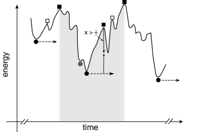
Figure 1: A fictitious time series of collected energy values illustrates our sampling procedure and our definition of a valley (= gray area). Conspicuous events, i.e. energy and barrier records, are denoted by circles and squares.

A discussion of the free energies associated with the fluctuation regime inside the valleys is left to forthcoming publications and the variable $t$ will denote the age of the system, except when otherwise indicated.

Method: A multitude of inequivalent metastable states produces the time inhomogeneous dynamics generally observed in aging systems. In most cases, these states are sets of configurations surrounding local energy minima, i.e., qualitatively speaking, valleys in the energy landscape. Since high-lying and shallow local energy minima greatly outnumber deep minima, the initial quench typically produces a poor local minimum and an aging system subsequently encounters a series of progressively higher energy barriers Sibani98 ; Joh99 ; Lederman91 which delimit progressively deeper valleys. The values of the highest barrier $B$ and lowest energy $E$—henceforth best so far or simply bsf barriers and energies—stand out as crucial events, and will serve to tag the valleys as they appear in the energy landscape.

The simulations start from a random, $T=\infty$, configuration and run at temperature $T$. Barrier values are computed as energy differences from the current bsf energy state. The bsf energy and barrier are initially $\infty$ and zero, respectively. Each run produces a time ordered sequence of $E$’s and $B$’s as e.g. $EBBEEBBBE$ in Fig. 1. Contiguous bsf energies pertain to a trajectory ‘tumbling’ down in a valley. Being mainly interested in the configuration where the tumbling stops, we only keep the lowest $E$ within each group. In Fig. 1 the datum removed is represented by the ‘$\otimes$’ symbol. Similarly, we want to avoid registering the numerous bsf barriers of roughly the same height which appear in close succession while the system goes through a high ‘saddle’. A barrier record is therefore kept only if the energy experiences a sufficiently deep local minimum before the next global barrier maximum is encountered. The precise definition of ‘sufficiently deep’ involves a positive number $x\leq 1$. For $x=1$, the local minimum must be as low as the current bsf energy, while for $x=0$ all bsf barriers are kept. Interestingly, our results are insensitive to the value of $x$ in the range $0.25-0.75$. In terms of Fig. 1, we only keep the full squares and circles, thereby reducing our string even further to its final state: $EBEBBE$.

For speed, we rely on the Waiting Time Method (WTM), a rejection-less Monte Carlo scheme Dall01 well suited for problems where $N$ variables contribute additively to the energy through local interactions. Based on the local field, each variable is stochastically assigned a flipping time and the variable with the shortest flipping time is updated together with the local fields affected by the move. The sequence of WTM moves equals in probability Dall01 the sequence of accepted moves in the Metropolis algorithm. The current flipping time, henceforth simply ‘time’, corresponds to a Metropolis sweep, and to the physical time of an experiment.

Results: We consider $L^{d}$ Ising spins placed on a regular lattice of linear size $L$ which interact via the Edwards-Anderson Hamiltonian Edwards75

$${\cal H}(\alpha)=-\frac{1}{2}\sum_{i,j}J_{ij}s_{i}^{(\alpha)}s_{j}^{(\alpha)}.$$ (1)

In this formula, $s_{i}^{(\alpha)}$ is the spin value at site $i$ for configuration $\alpha$, the couplings $J_{ij}$ are symmetric in their two indices and vanish unless $i$ and $j$ belong to neighbor sites. In the latter case they are drawn independently from a Gaussian distribution of unit variance. The dynamics is nearest neighbor thermal hopping with detailed balance. The runs spanned over several time decades, always bringing the system down to quite low energies, typically around $-1.66$ per spin. Large systems tend to have more shallow valleys than smaller system. To obtain meaningful comparisons all data originating from the first ten time units after the quench were discarded, and the value of the valley index was shifted up to one unit in our scaling plots in Figs. 3 and 4.

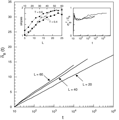
Figure 2: Main figure: the average number $\overline{n_{B}}$ of barrier records versus time for three selected system sizes in $2d$ at $T=0.4$. Left insert: the logarithmic slopes of $\overline{n_{B}}$ as a function of the linear system size $L$ for $2d$ ($T=0.4$ and $0.6$) and $3d$ ($T=0.4$). The upper (lower) scale refers to $2d$ ($3d$) systems. Right insert: the variance to average ratio for $n_{B}(t)$ for the data in the main figure.

A basic quantity is the number of events (barrier or energy records) which on average occur in $[0,t]$. Since achieving a record becomes increasingly difficult, the rate of events will decrease in time and the dynamics decelerates. Interestingly, a time homogeneous dynamics is restored by using the natural logarithm $\ln t$ as time variable. This is shown in Fig. 2, where the average number $\overline{n_{B}}(t)$ of barrier crossing events is plotted as a function of $\ln t$. The data shown in the main figure belong to $2d$ systems, while similar data in both $2d$ and $3d$ were omitted for clarity. The left insert shows the logarithmic rate of events $d\overline{n_{B}}(t)/d\ln t$, in $2d$ as well as $3d$, as a function of $L$. Finally, the right insert shows the ratio of the variance $\sigma^{2}_{n_{B}}(t)$ to $\overline{n_{B}}(t)$. Both quantities were estimated for $3000$ independent runs: The variance and the average follow the same logarithmic fashion, with the former trailing the latter due to an initial lag. A similar statistics is also approached by the number of bsf records—and hence the number of valleys—discovered on average in $[0,t]$, for sufficiently large systems. A logarithmic dependence of macroscopic averages is ubiquitous in complex metastable systems. Beside the present examples it is found in e.g. driven dissipative models Sibani01 , vibrated granular systems Jaeger89 ; Josserand00 , Lennard-Jones glasses Kob00 , nitridic ceramics Hannemann02 and population dynamics Sibani99 .

The approximate equality between average and variance points to the relevance of log-Poisson statistics describing the number of magnitude records achieved in a sequence of $t$ independent random numbers Sibani93a . The name stresses that $\ln t$, rather than $t$, is the relevant time variable. For data stemming from a nearest neighbor random walk in a landscape, log-Poisson statistics indicates a de-correlation of the energy function between consecutive barrier records, and a fortiori during the time spent within each valley. Since the correlation time and the relaxation time (for the internal thermalization) can be generically identified VanKampen92 , we conclude that thermal quasi-equilibrium is achieved within a valley. As a consequence, the morphology of quasi-equilibrium fluctuations around the bsf state of each valley can be isolated from the non-equilibrium dynamics and analyzed separately.

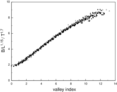
Figure 3: Average energy barriers records $B$ separating contiguous valleys in $3d$ spin glass landscapes are scaled with $L$ and $T$, as indicated in the ordinate label and plotted versus $n$. All combinations of $L=8,10,12,14,16$ and $T=0.3,0.4,0.5,0.6$ and $0.7$ are included, plus $L=18$ and $T=0.4$.

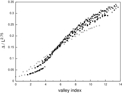
Figure 4: The average difference $\Delta$ between the lowest energies of the first and the $n$’th valley is plotted versus $n$. The ordinate is scaled with $L$ as indicated. The system and the combinations of $L$ and $T$ shown are as in Fig. 3, except for an additional $T=0.2$ data set (upper triangle), which falls outside the main trend. The remaining spread in the data collapse cannot be removed by introducing an additional scaling parameter, and is likely indicative of an underlying distribution of minima.

The scaling of the logarithmic rate of events with $L$ is shown in the left insert of Fig. 2 to increase from an initial value of $1$ to approximately $2$ for large system sizes. With Poisson statistics, this rate is proportional to the number of lattice ‘regions’ evolving independently. As the spins are quiescent most of the time, a record in one region leads to an overall record as well. Thus, two length scales Lamarcq02 might in principle coexist: the linear size of the quasi-equilibrium fluctuations and the extent of the non-equilibrium ‘earthquakes’ leading from one valley to the next. Figs. 2 and 4 imply that the latter scale is asymptotically $\propto L$, i.e. earthquakes are extensive or near extensive events. This is further confirmed by the distribution (not shown) of the Hamming distance (i.e. the number of spins whose orientations differ), between the bsf configurations of valleys $n$ and $n+1$. The distribution is exponential, and its average grows linearly in $n$ and close to linearly in $L^{d}$.

The scaling with $L$ and $T$ of the energy barrier $B$ separating two contiguous valleys in $3d$ systems is shown in Fig. 3. All points are quenched averages over $3000$ independent runs for the $L$ and $T$ values specified in the caption. As mentioned, the data have been shifted by up to one unit along the abscissa, which mirrors the arbitrariness of the initial bsf states—conventionally recorded after ten time units. As indicated in the plot, $B\propto L^{1.15}T^{1.7}$. We have not attempted a quantitative determination of the uncertainty on the scaling exponents, but changing the last significant digit visibly affects the quality of the plot.

The above considerations apply equally well to Fig. 4, which, for the same set of runs, depicts the average difference $\Delta(1,n)$ between the bsf energy of valley $1$ and $n$. $\Delta(1,n)$ is independent of $T$, as one should expect, and increases almost linearly with the valley index. Refs. Sibani91 ; Hoffmann97 analyze a mesoscopic model with this exact property. The curvature for large $n$ might partly be due to a systematic error, since not every run enters the last few valleys within the maximum time span allotted to the calculations. For very long time scales, the curve will approach the constant value of the difference between the first bsf energy and the energy of the ground state.

The strong $L^{2.75}$ size dependence of $\Delta(1,n)$ is noticeable: since moving from one valley to the other involves the rearrangements of ${\cal O}(L^{3})$ spins, it seems likely that the set difference between two bsf energy configurations be a sponge-like object of the sort discussed in Houdayer00 ; Lamarcq02 . The energy difference between different bsf states is clearly not ${\cal O}(1)$ as expected in mean-field. It seems unlikely that going to lower energies could radically change the scaling of $\Delta$ with system size. We stress again that the WTM and the Metropolis algorithm being equivalent, everything could have been done in the conventional way, albeit with much greater numerical effort.

In summary, the distinction between pseudo-equilibrium fluctuations and strongly non-equilibrium events in aging dynamics is emphasized. We link the latter events to barrier and energy records marking the appearance of new valleys as the landscape unfolds during aging. The homogeneity of the event statistics in $\ln t$ is explained theoretically in terms of the statistics of records.

The description of spin glass non-equilibrium dynamics as a log-Poisson process indicates that thermal aging can be treated on the same footing as driven dissipative dynamics Sibani93a ; Sibani01 and evolution models Sibani99a ; Hall02 , in spite of obvious differences at the microscopic level. It also implies that, on each time scale, glassy dynamics typically selects the least stable among the metastable configurations available. While this feature has been noticed in more restricted contexts Coppersmith87 ; Sibani93a ; Sibani01 , the present study suggests that it might provide a powerful and general paradigm for glassy relaxation.

Acknowledgments: PS is indebted to Greg Kenning and Henrik J. Jensen for discussions and to the Danish SNF for grant 23026.

References

- [1] M. Alba, M. Ocio, and J. Hammann, Europhys. Lett. 2, 45 (1986).
- [2] P. Svedlindh, P. Granberg, P. Nordblad, L. Lundgren, and H. Chen, Phys. Rev. B 35, 268 (1987).
- [3] J.-O. Andersson, J. Mattsson, and P. Svedlindh, Phys. Rev. B 46, 8297 (1992).
- [4] D. S. Fisher and D. A. Huse, Phys. Rev. B 38, 373 (1988).
- [5] G. Koper and H. Hilhorst, Journal de Physique 49, 429 (1988).
- [6] P. Sibani and K. H. Hoffmann, Phys. Rev. Lett. 63, 2853 (1989).
- [7] P. Sibani and K. Hoffmann, Europhys. Lett. 16, 423 (1991).
- [8] Y. G. Joh and R. Orbach, Phys. Rev. Lett. 77, 4648 (1996).
- [9] K. Hoffmann, S. Schubert, and P. Sibani, Europhys. Lett. 38, 613 (1997).
- [10] J. Bouchaud, J. Phys. I France 2, 1705 (1992).
- [11] S. Coppersmith and P. Littlewood, Phys. Rev. B 36, 311 (1987).
- [12] P. Sibani and P. B. Littlewood, Phys. Rev. Lett. 71, 1482 (1993).
- [13] P. Sibani and C. M. Andersen, Phys. Rev. E 64, 021103, 1 (2001).
- [14] K. Jonason, E. Vincent, J. Hamman, J. P. Bouchaud, and P. Nordblad, Phys. Rev. Lett. 81, 3243 (1998).
- [15] F. H. Stillinger and T. A. Weber, Phys. Rev. A 28, 2408 (1983).
- [16] K. Nemoto, J. Phys. A 21, L287 (1988).
- [17] O. M. Becker and M. Karplus, J. Chem. Phys. 106, 1495 (1997).
- [18] S. Mossa, G. Ruocco, F. Sciortino, and P. T. P, Phil. Mag. B 82, 695 (2002).
- [19] A. Crisanti and F. Ritort, J. of Phys. Cond. Matt. 14, 1381 (2002).
- [20] M. Palassini and A. P. Young, Phys. Rev. Lett. 83, 5126 (1999).
- [21] J. Houdayer and O. C. Martin, Europhys. Lett. 49(6), 794 (2000).
- [22] J. Lamarcq, J. P. Bouchaud, O. C. Martin, and M. Mezard, Europhys. Lett. 58, 321 (2002).
- [23] P. Sibani, Physica A 258, 249 (1998).
- [24] Y. G. Joh, R. Orbach, G. G. Wood, J. Hammann, and E. Vincent, Phys. Rev. Lett. 82, 438 (1999).
- [25] M. Lederman, R. Orbach, J. Hammann, M. Ocio, and E. Vincent, Phys. Rev. B 44, 7403 (1991).
- [26] J. Dall and P. Sibani, Comp. Phys. Comm. 141, 260 (2001).
- [27] S. F. Edwards and P. W. Anderson 5, 965 (1975).
- [28] H. M. Jaeger, C. heng Liu, and S. R. Nagel, Phys. Rev. Lett. 62, 40 (1989).
- [29] C. Josserand, A. V. Tkachenko, D. M. Mueth, and H. M. Jaeger, Phys. Rev. Lett. 85, 3632 (2000).
- [30] W. Kob, F. Sciortino, and P. Tartaglia, Europhys. Lett. 49, 590 (2000).
- [31] A. Hannemann, J. C. Schön, M. Jansen, and P. Sibani, cond-mat/0212245 (2002).
- [32] P. Sibani, R. van der Pas, and J. C. Schön, Computer Physics Communications 116, 17 (1999).
- [33] N. G. V. Kampen, Stochastic Processes in Physics and Chemistry (North Holland, 1992).
- [34] P. Sibani and A. Pedersen, Europhys. Lett. 48, 346 (1999).
- [35] M. Hall, K. Christensen, S. A. di Collabiano, and H. J. Jensen, Phys. Rev. E 66, 011904 (2002).