Magnon-Mediated Superconductivity in Itinerant Ferromagnets

Abstract

The present paper discusses magnon-mediated superconductivity in ferromagnetic metals. The mechanism explains in a natural way the fact that the superconductivity in $UGe_{2}$, $ZrZn_{2}$ and $URhGe$ is apparently confined to the ferromagnetic phase.The order parameter is a spin anti-parallel component of a spin-1 triplet with zero spin projection. The transverse spin fluctuations are pair forming and the longitudinal ones are pair breaking.The competition between magnons and paramagnons explains the existence of two successive quantum phase transitions in $UGe_{2}$, from ferromagnetism to ferromagnetic superconductivity, and at higher pressure to paramagnetism. The maximum $T_{SC}$ results from the suppression of the paramagnon contribution. To form a Cooper pair an electron transfers from one Fermi surface to the other. As a result, the onset of superconductivity leads to the appearance of two Fermi surfaces in each of the spin up and spin down momentum distribution functions. This fact explains the linear temperature dependence at low temperature of the specific heat, and the experimental results for $UGe_{2}$.

74.20.Mn, 75.50.Cc, 74.20.Rp, 75.10.Lp

The discovery of superconductivity in a single crystal of $UGe_{2}$[2, 3], $ZrZn_{2}$[4] and $URhGe$[5] revived the interest in the coexistence of superconductivity and ferromagnetism. The experiments indicate that in very pure systems, and at very low temperature, ferromagnetism and superconductivity can coexist, with the same electrons that cause the magnetism also responsible for the superconductivity. The superconductivity is apparently confined to the ferromagnetic phase. There are two successive quantum phase transitions in $UGe_{2}$[2, 3], from ferromagnetism to ferromagnetic superconductivity, and at higher pressure to paramagnetism. The specific heat anomaly associated with the superconductivity appears to be absent and the specific heat depends linearly on the temperature at low temperature[6, 4, 5].

The paramagnon-mediated superconductivity [7, 8] has long been considered the most promising theory of coexistence of superconductivity and ferromagnetism.The order parameters are spin parallel components of the spin triplet. The superconductivity in $ZrZn_{2}$ was predicted. Nevertheless, the theory meets some difficulties. It predicts that the superconductivity occurs in both the ferromagnetic and the paramagnetic phases. A solution of the problem was recently proposed. It has been shown[9] that the critical temperature is much higher in the ferromagnetic phase than in the paramagnetic one due to the coupling of the magnons to the longitudinal spin fluctuations. Alternatively, the superconductivity in the ferromagnetic state of $ZrZn_{2}$ is explained in [10] as a result of an exchange-type interaction between the magnetic moments of triplet-state Cooper pairs and the ferromagnetic magnetization density in the Ginzburg-Landau mean field theory. The Fay and Apple (FA) theory predicts that spin up and spin down fermions form Cooper pairs, and hence the specific heat decreases exponentially at low temperature. The phenomenological theories [11, 12] circumvent the problem assuming that only majority spin fermions form pairs, and hence the minority spin fermions contribute the asymptotic of the specific heat. The coefficient $\gamma=\frac{C}{T}$ is twice smaller in the superconducting phase, which closely matches the experiments with $URhGe$[5]. But the assumption is quite questionable when the magnetization approaches zero. The superconducting critical temperature in (FA) theory increases when the magnetization decreases and very close to the quantum critical point falls down rapidly. It has recently been the subject of controversial debate. It is obtained in[13], by means of a more complete Eliashberg treatment, that the transition temperature is nonzero at the critical point. In [14], however, the authors have shown that the reduction of quasiparticle coherence and life-time due to spin fluctuations is the pair-breaking process which leads to a rapid reduction of the superconducting critical temperature near the quantum critical point. Finally, recent studies of polycrystalline samples of UGe2 show that T-P phase diagram is very similar to those of single-crystal specimens of UGe2 [15]. These findings suggest that the superconductivity in UGe2 is relatively insensitive to the presence of impurities and defects which excludes the spin parallel pairing.

In the present paper an itinerant system is considered in which the spin-$\frac{1}{2}$ fermions responsible for the ferromagnetism are the same quasiparticles which form the Cooper pairs. The interaction of quasiparticles $c_{\sigma}(\vec{x})(c^{+}_{\sigma}(\vec{x}))$ with spin fluctuations has the form

$$H_{\text{s-f}}=J\int d^{3}x\,c^{+}(\vec{x})\frac{\vec{\tau}}{2}c(\vec{x})\cdot\vec{M}(\vec{x})$$ (1)

where the transverse spin fluctuations are described by magnons $M_{1}(\vec{x})+iM_{2}(\vec{x})=\sqrt{2M}a(\vec{x})$, $M_{1}(\vec{x})-iM_{2}(\vec{x})=\sqrt{2M}a^{+}(\vec{x})$ and the longitudinal spin fluctuations by paramagnons $M_{3}(\vec{x})-M=\varphi(\vec{x})$. $M$ is zero temperature dimensionless magnetization of the system per lattice site. The magnon’s dispersion is $\omega(\vec{k})=\rho\vec{k}^{2}$ where the spin stiffness constant is proportional to $M$ ($\rho=M\rho_{0}$), and the paramagnon propagator is

$$D_{\text{pm}}=\frac{1}{r-i\frac{\omega}{|\vec{p}|}+b\vec{p}^{2}}.$$ (2)

The parameter $r$ is the inverse static longitudinal magnetic susceptibility, which measures the deviation from quantum critical point. The constants $J,\rho_{0}$ and $b$ are phenomenological ones subject to some relations.

Integrating out the spin fluctuations one obtains an effective four fermion theory which can be written as a sum of four terms. Three of them describe the interaction of the components of spin-1 composite fields $(\uparrow\uparrow,\uparrow\downarrow+\downarrow\uparrow,\downarrow\downarrow)$ which have a projection of spin 1,0 and -1 respectively. The fourth term describes the interaction of the spin singlet composite fields $\uparrow\downarrow-\downarrow\uparrow$. The spin singlet fields’ interaction is repulsive and does not contribute to the superconductivity [16]. The spin parallel fields’ interactions are due to the exchange of paramagnons and do not contribute to the magnon-mediated superconductivity. The relevant interaction is that of the $\uparrow\downarrow+\downarrow\uparrow$ fields. In static approximation, the Hamiltonian of interaction is

$$H_{\text{i}nt}=-\frac{J^{2}}{16}\int\prod\limits_{i}\frac{d^{3}k_{i}}{(2\pi)^{3}}\left[c_{\uparrow}^{+}(\vec{k}_{1})c_{\downarrow}^{+}(\vec{k}_{2})+c_{\downarrow}^{+}(\vec{k}_{1})c_{\uparrow}^{+}(\vec{k}_{2})\right]$$ (3)

(4)

$$\left[c_{\uparrow}(\vec{k}_{2}-\vec{k}_{3})c_{\downarrow}(\vec{k}_{1}+\vec{k}_{3})+c_{\downarrow}(\vec{k}_{2}-\vec{k}_{3})c_{\uparrow}(\vec{k}_{1}+\vec{k}_{3})\right]V(\vec{k}_{3})$$ (5)

where the potential

$$V(\vec{k})=\frac{2M}{\rho\vec{k}^{2}}-\frac{1}{r+b\vec{k}^{2}}$$ (6)

has an attracting part due to exchange of magnons and a repulsive part due to exchange of paramagnons. The effective Hamiltonian of the system is

$$H_{\text{e}ff}=H_{0}+H_{\text{i}nt}$$ (7)

where $H_{0}$ is the Hamiltonian of the free spin up and spin down fermions with dispersions

$$\epsilon_{\uparrow}(\vec{k}) = \frac{\vec{k}^{2}}{2m}-\mu-\frac{JM}{2},$$ (8)

$$\epsilon_{\downarrow}(\vec{k}) = \frac{\vec{k}^{2}}{2m}-\mu+\frac{JM}{2}$$ (9)

One can obtain the gap equation following the standard technique. To ensure that the fermions which form Cooper pairs are the same as those responsible for spontaneous magnetization, one has to consider the equation for the magnetization

$$M=\frac{1}{2}<c^{+}_{\uparrow}c_{\uparrow}-c^{+}_{\downarrow}c_{\downarrow}>$$ (10)

as well. Then the system of equations for the gap and for the magnetization determines the phase where the superconductivity and the ferromagnetism coexist.The system can be written in terms of Bogoliubov excitations, which have the following dispersions relations:

$$E_{1}(\vec{k})=-\frac{JM}{2}-\sqrt{\epsilon^{2}(\vec{k})+|\Delta(\vec{k})|^{2}}$$ (11)

$$E_{2}(\vec{k})=\frac{JM}{2}-\sqrt{\epsilon^{2}(\vec{k})+|\Delta(\vec{k})|^{2}}$$ (12)

where $\Delta(\vec{k})$ is the gap, and $\epsilon(\vec{k})=\frac{\vec{k}^{2}}{2m}-\mu$.

At zero temperature the equations take the form

$$M = \frac{1}{2}\int\frac{d^{3}k}{(2\pi)^{3}}\left[1-\Theta(-E_{2}(\vec{k}))\right]$$ (13)

$$\Delta(\vec{p}) = \frac{J^{2}}{8}\int\frac{d^{3}k}{(2\pi)^{3}}\,\frac{V(\vec{p}-\vec{k})\,\,\Theta(-E_{2}(\vec{k}))}{\sqrt{\epsilon^{2}(\vec{k})+|\Delta(\vec{k})|^{2}}}\,\Delta(\vec{k})$$ (14)

The gap is an antisymmetric function $\Delta(-\vec{k})=-\Delta(\vec{k})$, so that the expansion in terms of spherical harmonics $Y_{lm}(\Omega_{\vec{k}})$ contains only terms with odd $l$. I assume that the component with $l=1$ and $m=0$ is nonzero and the other ones are zero

$$\Delta(\vec{k})=\Delta_{10}(k)\sqrt{\frac{3}{4\pi}}\cos\theta.$$ (15)

Expending the potential in terms of Legendre polynomial $P_{l}$ one obtains that only the component with $l=1$ contributes the gap equation. The potential $V_{1}(p,k)$ has the form,

$$V_{1}(p,k) = \frac{3M}{\rho}\left[\frac{p^{2}+k^{2}}{4p^{2}k^{2}}\ln\left(\frac{p+k}{p-k}\right)^{2}-\frac{1}{pk}\right]-$$ (17)

$$\frac{3M}{\rho}\beta\left[\frac{p^{2}+k^{2}}{4p^{2}k^{2}}\ln\frac{r^{\prime}+(p+k)^{2}}{r^{\prime}+(p-k)^{2}}\,-\,\frac{1}{pk}\right],$$

where $\frac{3M}{\rho}=\frac{3}{\rho_{0}}$, $\beta=\frac{\rho}{2Mb}=\frac{\rho_{0}}{2b}>1$ and $r^{\prime}=\frac{r}{b}<<1$. A straightforward analysis shows that for a fixed $p$ , the potential is positive when $k$ runs an interval around $p$ $(p-\Lambda,p+\Lambda)$, where $\Lambda$ is approximately independent on $p$. In order to allow for an explicit analytic solution, I introduce further simplifying assumptions by neglecting the dependence of $\Delta_{10}(k)$ on $k$ ($\Delta_{10}(k)=\Delta_{10}(p_{f})=\Delta$) and setting $V_{1}(p_{f},k)$ equal to a constant $V_{1}$ within interval $(p_{f}-\Lambda,p_{f}+\Lambda)$ and zero elsewhere. The system of equations (13,14) is then reduced to the system

$$M = \frac{1}{8\pi^{2}}\int\limits_{0}^{\infty}dkk^{2}\int\limits_{-1}^{1}dt[1-\Theta(-E_{2}(k,t))]$$ (18)

$$\Delta = \frac{J^{2}V_{1}}{32\pi^{2}}\int\limits_{p_{f}-\Lambda}^{p_{f}+\Lambda}dkk^{2}\int\limits_{-1}^{1}dt\,t^{2}\frac{\Theta(-E_{2}(k,t))}{\sqrt{\epsilon^{2}(k)+\frac{3}{4\pi}t^{2}\Delta^{2}}}\Delta$$ (19)

where $t=\cos\theta$.

One looks for a solution of the system which satisfies $\sqrt{\frac{3}{\pi}}\Delta<JM$. Then the equation $E_{2}(k,t)=0$ defines the Fermi surfaces

$$k^{\pm}_{f}=\sqrt{p^{2}_{f}\pm m\sqrt{J^{2}M^{2}-\frac{3}{\pi}t^{2}\Delta^{2}}}\,\,,\,\,\,p_{f}=\sqrt{2\mu m}$$ (20)

The domain between the Fermi surfaces contributes to the magnetization $M$ in Eq.(18), but it is cut out from the domain of integration in the gap equation Eq.(19). One is primarily interested in determining at what magnetization a superconductivity exists. When the magnetization increases, the domain of integration in the gap equation decreases. Near the quantum critical point the size of the gap is small, and hence the linearized gap equation can be considered. Then it is easy to obtain the critical value of the magnetization $M_{SC}$

$$M_{SC}=\frac{4p^{2}_{f}}{mJ}\left(1+\frac{4p^{2}_{f}-\Lambda^{2}}{\Lambda^{2}}\exp\left[\frac{64\pi^{2}}{3J^{2}V_{1}mp_{f}}\right]\right)^{-\frac{1}{2}}$$ (21)

Near the second quantum phase transition, when the magnetization approaches zero, the domain between the Fermi surfaces decreases. One can approximate the equation for magnetization Eq.(18) substituting $k^{\pm}_{f}$ from Eq.(20) in the the difference $(k^{+}_{f})^{2}-(k^{-}_{f})^{2}$ and setting $k^{\pm}_{f}=p_{f}$ elsewhere. Then, in this approximation, the magnetization is linear in $\Delta$, namely

$$\Delta=\sqrt{\frac{\pi}{3}}J\kappa M$$ (22)

where $\kappa$ runs the interval $(0,1)$, and satisfies the equation

$$\kappa\sqrt{1-\kappa^{2}}+\arcsin\kappa\,=\frac{8\pi^{2}}{mp_{f}J}$$ (23)

The Eq.(23) has a solution if $mp_{f}J>16\pi$. Substituting $M$ from Eq.(22) in Eq.(19), one arrives at an equation for the gap. This equation can be solved in a standard way and the solution is

$$\Delta = \sqrt{\frac{16\pi}{3}}\frac{\Lambda p_{f}\kappa}{m}\exp\left[-\frac{3}{2}I(\kappa)-\frac{24\pi^{2}}{J^{2}V_{1}mp_{f}}\right]$$ (24)

$$I(\kappa) = \int\limits_{-1}^{1}dtt^{2}\ln\left(1+\sqrt{1-\kappa^{2}t^{2}}\right)$$ (25)

Eqs (22,23,24) are the solution of the system Eqs.(18,19) near the quantum transition to paramagnetism.

When superconductivity and ferromagnetism coexist, the momentum distribution functions $n^{\uparrow}(p,t)$ and $n^{\downarrow}(p,t)$ of the spin-up and spin-down quasiparticles have two Fermi surfaces each. One can write them in terms of the distribution functions of the Bogoliubov fermions

$$n^{\uparrow}(p,t) = u^{2}(p,t)n_{1}(p,t)+v^{2}(p,t)n_{2}(p,t)$$ (26)

$$n^{\downarrow}(p,t) = u^{2}(p,t)(1-n_{1}(p,t))+v^{2}(p,t)(1-n_{2}(p,t))$$ (27)

where $u(p,t)$ and $v(p,t)$ are the coefficients in the Bogoliubov transformation. At zero temperature $n_{1}(p,t)=1$, $n_{2}(p,t)=\Theta(-E_{2}(p,t))$, and the Fermi surfaces Eq.(20) manifest themselves both in the spin-up and spin-down momentum distribution functions. The functions are depicted in Fig.1 and Fig.2.

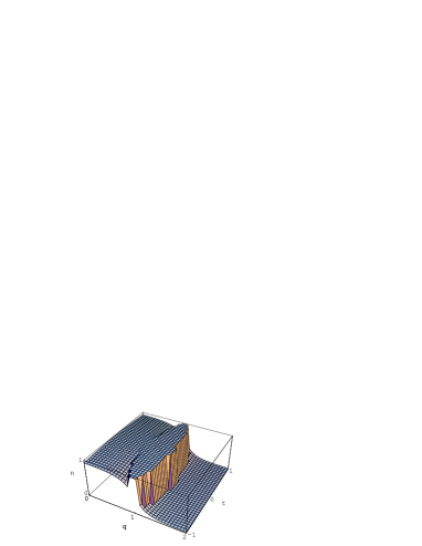
FIG. 1.: The zero temperature momentum distribution $n$, for spin up fermions, as a function of $q=\frac{p}{p_{f}}$ and $t=\cos\theta$.

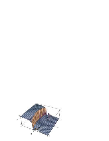
FIG. 2.: The zero temperature momentum distribution $n$, for spin down fermions, as a function of $q=\frac{p}{p_{f}}$ and $t=\cos\theta$.

The two Fermi surfaces are necessary for the existence of itinerant ferromagnetism , and explain the mechanism of Cooper pairing. In the ferromagnetic phase $n^{\uparrow}$ and $n^{\downarrow}$ have different (majority and minority) Fermi surfaces. To form a spin anti-parallel Cooper pair, the fermion has to transfer from one Fermi surface to the other. If the value of the momentum of the emitted or absorbed magnon lies in the domain where the effective potential is attracting but outside the domain between the two Fermi surfaces, fermions with opposite spins form a Cooper pair. As a result, the onset of superconductivity is accompanied by the appearance of a second Fermi surface in each of the spin-up and spin-down momentum distribution functions.

The existence of the two Fermi surfaces also explains the linear dependence of the specific heat at low temperatures as opposed to the exponential decrease of the specific heat in the BCS theory:

$$\frac{C}{T}\,=\,\frac{2\pi^{2}}{3}\left(N^{+}(0)+N^{-}(0)\right)$$ (28)

Here $N^{\pm}(0)$ are the density of states on the Fermi surfaces. One ca rewrite the $\gamma=\frac{C}{T}$ constant in terms of Elliptic Integral of the second kind $E(\alpha,x)$

$$\gamma\,=\,\frac{mp_{f}}{3\kappa} \left[(1+s)^{\frac{1}{2}}E(\frac{1}{2}\arcsin\kappa,\frac{2s}{s+1})+\right.$$ (30)

$$\left.(1-s)^{\frac{1}{2}}E(\frac{1}{2}\arcsin\kappa,\frac{2s}{s-1})\right].$$

where $s=\frac{JMm}{p^{2}_{f}}<1$ and $\kappa=\sqrt{\frac{3}{\pi}}\frac{\Delta}{JM}$. The Eq.(30) shows that in the ferromagnetic phase ($\Delta=0$) the specific heat constant $\gamma$ is smaller than in the superconducting one, which closely matches the experiments with $UGe_{2}$[6]. Important point is that UGe2 is an anisotropic ferromagnet and hence the magnon has a gap which changes the potential Eq.(17). The physical consequence of the change is that the superconductivity disappears before the quantum phase transition from ferromagnetism to paramagnetism (see [6, 15]). The distance between these two points depends on the anisotropy.

The presence of an additional phase line $T_{x}$ and the correlation between a transition at $T_{x}$ and the appearance of superconductivity in $UGe_{2}$ has been proved [3, 6]. It lies entirely within the ferromagnetic phase and is suggested by a strong anomaly in the resistivity at a temperature $T_{x}$. The maximum transition temperature for superconductivity is near the pressure $P_{x}$ where $T_{x}$ vanishes. The authors have assumed that superconductivity is mediated by fluctuations associated with a (hypothetical) second order critical point $P_{x}$, with an unidentified order parameter.

Experimental measurement of ac magnetic susceptibility as a function of the temperature indicates a peak at ferromagnetic Curie temperature, as usual. But the peak is substantially damped at a pressure near the maximal superconducting critical temperature [17]. The suppression of the peak can be understood as a suppression of the paramagnon contribution, which in turn means suppression of pair-breaking effects and hence higher superconducting critical temperature. So the proposed model of magnon mediated superconductivity complemented by the experimental results explains, at least qualitatively, the superconductivity in $UGe_{2}$ without invoking an additional phase transition.

The proposed model of ferromagnetic superconductivity differs from the models discussed in [7, 8, 9, 10, 11, 12] in two ways. First, the superconductivity is due to the exchange of magnons, and paramagnons have pair-breaking effect. Second, the order parameter is a spin antiparallel component of a spin triplet with zero spin projection. The existence of two Fermi surfaces in each of the spin-up and spin-down momentum distribution functions is a generic property of a ferromagnetic superconductivity with spin anti-parallel pairing (see also[18]). They lead to a linear temperature dependence of the specific heat at low temperature. But the experimental result has an alternative theoretical explanation in [5, 11, 12]. So, one needs an experiment which proves undoubtedly the existence of the predicted Fermi surfaces.

The author would like to thank C. Pfleiderer and R.Rashkov for valuable discussions.

REFERENCES

- [1] Electronic address: naoum@phys.uni-sofia.bg
- [2] S. Saxena, et al., Nature (London) 406, 587 (2000).
- [3] A. Huxley, et al., Phys. Rev. B 63, 144519 (2001).
- [4] C. Pfleiderer, et al., Nature (London) 412, 58 (2001).
- [5] D. Aoki,et al., Nature (London) 413, 613 (2001).
- [6] N. Tateiva, et al., J. Phys. Condens. Matter 13, L17 (2001).
- [7] C. P. Enz, and P. T. Matthias, Science 201, 828 (1978).
- [8] D. Fay, and J. Apple, Pys.Rev. B 22, 3173 (1980).
- [9] T. Kirkpatrick, D. Belitz, T. Vojta and R. Narayanan Phys. Rev. Lett. 87, 127003 (2001).
- [10] M. B. Walker, and K. V. Samokhin, Phys. Rev. Lett. 88, 207001 (2002).
- [11] K. Machida, and T. Ohmi, Phys. Rev. Lett.86, 850 (2001).
- [12] I. A. Fomin, JETP Lett.74, 116 (2001).
- [13] R. Roussev and A.Millis, Phys. Rev. B 63, 140504 (2001).
- [14] Z. Wang, W. Mao, and K. Bedell, Phys. Rev. Lett. 87, 257001 (2001).
- [15] E. Bauer, et al., J. Phys. Condens. Matter 13 L759 (2001).
- [16] N. F. Berk, and J. R Schrieffer, Phys. Rev. Lett. 17, 433 (1966).
- [17] G. Motoyama, S. Nakamura, H. Kadoya, T. Nishioka, and N. Sato, Phys. Rev. B 65, 020510(R) (2001).
- [18] N. Karchev, K. Blagoev, K. Bedell, and P. Littlewood, Phys. Rev. Lett., 86 846 (2001).