Lattice-model study of the thermodynamic interplay of polymer crystallization and liquid-liquid demixing

Abstract

We report Monte Carlo simulations of a lattice-polymer model that can account for both polymer crystallization and liquid-liquid demixing in solutions of semiflexible homopolymers. In our model, neighboring polymer segments can have isotropic interactions that affect demixing, and anisotropic interactions that are responsible for freezing. However, our simulations show that the isotropic interactions also have a noticeable effect on the freezing curve, as do the anisotropic interactions on demixing. As the relative strength of the isotropic interactions is reduced, the liquid-liquid demixing transition disappears below the freezing curve. A simple, extended Flory-Huggins theory accounts quite well for the phase behavior observed in the simulations.

I Introduction

Lattice models of polymer solutions are widely used because of their simplicity and computational convenience. [1, 2, 3, 4, 5, 6, 7, 8] When modeling a polymer solution, the polymer chain occupies consecutive sites on the lattice, each site corresponding to the size of one chain unit, while the remaining sites correspond to solvent.

The use of lattice models for polymer solutions dates back to the work of Meyer [1]. Flory [2] and Huggins [3] showed how, using a mean-field approximation, the lattice model yielded a powerful tool to predict the solution properties of flexible [9, 10, 11] and semi-flexible [7] polymers. Various refinements to the Flory-Huggins (F-H) model have been proposed by a number of authors (see, e.g. Refs. 4 to 6). FH-style models can account for liquid-liquid (L-L) phase separations with an upper critical solution temperature (UCST) driven by the site-to-site mixing pair interactions in polymer solutions - however, they are ill suited to describe polymer crystallization, i.e. liquid-solid (L-S) phase transitions. This limitation is not due to any intrinsic drawback of polymer lattice models as such, but to specific choice for the polymer interactions in the original F-H theory. In fact, the factors that lead to polymer crystallization, i.e. interactions that favor compact packing and stiffness of the polymer chains, can be accounted for in a lattice model, by introducing anisotropic interactions between adjacent polymer bonds. [8] Clearly, in real polymer solutions, both crystallization and phase separation can occur on cooling. While lattice models for polymer solutions can account for both types of phase transitions, most theoretical and simulation studies have focused on one transition or the other, and less attention has been paid to their interplay. Such interplay may change the pathway of a phase transition [12, 13] and hence determine the complex structure-property relationships of mixtures containing crystallizable polymers, which has been the subject of much experimental research dating back to Richards. [14]

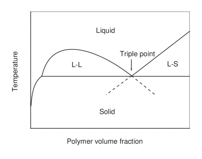
FIG. 1.: Schematic phase diagram of a binary mixture with a conventional monotectic triple point.

When the L-S phase-transition curve intersects the L-L coexistence curve, both curves are terminated at the resulting triple point. Below the triple point, the fluid phase may phase-separate into a dilute solution and a dense crystalline phase, as depicted in Fig.1. This combination of L-L demixing and crystallization is often referred to as “monotectic” behavior and has been observed in many experiments. [10, 15, 16] The morphology of polymer crystallites appears to be sensitive to the result of thermodynamic competition on cooling.[17] Special attention has been focused on the monotectic triple point. The kinetic competition between L-L demixing and crystallization on cooling in the vicinity of this triple point is an important issue for sol-gel transition and membrane preparation. [18, 19, 20] On cooling through the triple point, L-L phase separation is expected to occur before crystallization, though both phase transitions have the same equilibrium temperatures.[21] As a consequence, the density modulation produced during the early stage of L-L demixing may be frozen by subsequent crystallization. [22] Such frozen-in density modulations can be a practical way to control the metastable morphology of polymer gels and membranes through thermally induced processes. Therefore, the ability to predict phase diagrams of the type shown in Fig. 1 could be of considerable practical importance.

In this paper, we study the interplay of polymer crystallization and L-L demixing using both mean-field theories and Monte Carlo simulations of simple lattice models. In particular, we pay attention to the shift of the crystallization and L-L demixing curves in the phase diagrams due to this interplay.

The remainder of this paper is organized as follows: after an introductory description of the simulation techniques, we compare the simulation results with the relevant theoretical predictions for the L-L phase separation curve without prior disorder-order phase transition on cooling. Next, we discuss the simulations and mean-field calculation of the L-S curves and its thermodynamic competition with L-L demixing.

II Simulation Techniques

In our Monte Carlo simulations, we used a single-site-jumping micro-relaxation model with local sliding diffusion [23] to model the time evolution of self- and mutually-avoiding polymers in a cubic lattice with periodic boundary conditions. In this model, monomer displacements are allowed along both the cubic axes and the (body and face) diagonals, so the coordination number of each site includes all the neighboring sites along the main axes and the diagonals, and is $q=6+8+12=26$. The single-site jumping model with either kink generation or end-to-end sliding-diffusion was first proposed by Larson et al.[24] The kink-generation algorithm was subsequently developed into the bond-fluctuation model.[25, 26] A hybrid model combining kink generation and sliding diffusion into one mode of chain motion, was suggested by Lu and Yang.[27] The present hybrid model considers sliding-diffusion moves that are terminated by smoothing out the nearest kink conformation along the chain,[23] in accord with de Gennes’s picture of defect diffusion along the chain.[28] It has been verified that this model correctly reproduces both static and dynamic scalings of short polymers in the melt.[29]

In our simulations, we consider systems containing a number of $32$-unit polymer chains. The polymers reside in a cubic box with $32^{3}$ lattice sites. The polymer concentration was varied by changing the number of polymers in the simulation box. Monte Carlo sampling was performed using the Metropolis method. Three energetic parameters were used to model the intra- and inter-molecular interactions of the polymers. The first parameter $E_{c}$ measures the energy penalty associated with having two non-collinear consecutive bonds (a “kink”) along the chain; it is a measure of the rigidity of chains. The second parameter $E_{p}$ measures the energy difference between a pair of parallel and non-parallel polymer bonds in adjacent, non-bonded positions. A positive value of $E_{p}$ favors the compact packing of parallel chain molecules in a crystal. Finally, the parameter $B$ describes the energy penalty for creating a monomer-solvent contact. The total change in potential energy associated with a Monte Carlo trial move is

$$\frac{\Delta E}{k_{B}T} = \frac{E_{c}\Delta c+E_{p}\Delta p+B\Delta m}{k_{B}T}$$ (1)

$$= (\Delta c+\Delta p\frac{E_{p}}{E_{c}}+\Delta m\frac{B}{E_{c}})\frac{E_{c}}{k_{B}T},$$ (2)

where $\Delta c$ denotes the net change in the number of kinks, $\Delta p$ is the change in the number of non-parallel adjacent bonds, and $\Delta m$ measures the change in the number of monomer-solvent contacts. $k_{B}$ is the Boltzmann constant and $T$ is the temperature. As shown in Eq. 2, three dimensionless parameters control the acceptance probability of Monte Carlo trial moves: $B/E_{c}$ is the term that dominates the L-L demixing temperature but no effect at all on the freezing of the pure polymer system. In contrast, $E_{p}/E_{c}$ completely determines the freezing temperature of the pure polymer system, but it has only a slight effect on the demixing temperature. In fact, from Eq. 12 below, it follows that, the critical demixing temperature is approximately a factor of $q$ higher in the case $E_{p}=0$ and $B/E_{c}\neq 0$ than in the case where the values of $B$ and $E_{p}$ are interchanged. In what follows, $E_{c}/(k_{B}T)$ is used as a measure of the (inverse) temperature of the system. If $E_{c}$ is much larger than $B$ and $E_{p}$ , the polymer chains behave as almost rigid rods. In contrast, if $E_{c}=0$, the polymers are fully flexible. In what follows, we chose $E_{p}/E_{c}=1$ as a value typical for semiflexible chains. The choice of the value of $B/E_{c}$ (and thereby the L-L demixing region) is discussed in the following sections. In our simulations, we lowered the temperature by increasing the value of $E_{c}/(k_{B}T)$ from zero in steps of $0.002$. At each step, the total number of trial moves was $500$ MC cycles, where one Monte Carlo cycle (MC cycle) is defined as one trial move per monomer. The first $400$ MC cycles at each temperature were discarded for equilibration, after which samples were taken once per MC cycle and averaged. This process corresponds to a slow cooling of the sample system.

The most direct way to establish the equilibrium phase diagram of this model system would be to compute the free energy of all phases. Here, we follow a different route: we attempt to locate the equilibrium phase-transition temperatures during the dynamic cooling process. However, rapid cooling may lead to a significant supercooling mainly due to the presence of a free-energy barrier for homogeneous nucleation. This is particularly true in dilute solutions and small systems. In order to identify the correct equilibrium coexistence curves in a dynamic cooling scheme, supercooling should be eliminated as much as possible. To this end, we introduced one solid layer of terraced substrate formed by extended chains, as shown in Fig. 2A. These terraces can induce heterogeneous nucleation with a very small free-energy barrier. On such a large, terraced substrate, layer-by-layer crystal growth can take place directly, thereby obviating the need for homogeneous nucleation. In order to increase the accuracy of the method near the onset of the phase transition, we monitored the properties of the system during successive blocks of $500$ MC cycles. If, during such a block, we found evidence for the onset of a phase transition, we kept the temperature constant for a number of subsequent blocks, until no further drift in the system properties was observed.

On cooling, the degree of order in the sample system can be traced by the Flory “disorder” parameter, defined as the mean fraction of non-collinear connections of two consecutive bonds along the chains. On the cubic lattice, where $24$ out of $25$ directions for the connection to the next bond are non- collinear, the high-temperature limit of the disorder parameter is $0.96$. The degree of demixing of the system can be monitored by tracing the value of a “mixing” parameter, defined as the mean fraction of the sites around a chain unit, that are occupied by solvent. Our estimates of the onsets of phase transitions are based on the averaged results of five independent cooling processes characterized by the same energy parameters, but different seeds for the random-number generation.

A.

B.

C.

D.

FIG. 2.: Effect of a terraced substrate on the onset of crystallization upon cooling. The figures shown above were obtained for a solution of model polymers with length $r=32$, at a volume fraction $\phi=0.0625$, with $E_{p}/E_{c}=1$ and $B/E_{c}=0$. (A) Snapshot of an athermal sample system containing one layer of terraced substrate formed by extended chains, that are not included in the polymer volume fraction. Viewing along the extended chains. (B) Disorder-parameter cooling curves for the sample systems with a terraced substrate on cooling (solid line) and under the absence of a seed on cooling (dashed line). The arrow indicates the onset of phase transition. (C) Step-size dependence of the onset of crystallization on cooling. (D) Finite-size scaling of the onset of crystallization on cooling for the sample systems with denoted concentrations. All error bars are smaller than the symbols. The segments are drawn as a guide to the eye.

As can be seen from Fig. 2B, the presence of a terraced substrate significantly decreases the kinetic delay on cooling for polymer crystallization from a dilute solution. The onset of crystallization induced by the terraced substrate becomes insensitive to the number of steps on the substrate when this number is larger than $8$, see Fig. 2C. One might expect that more steps on the substrate would cause the substrate to adsorb more chains. The fact that the phase-transition temperature becomes insensitive to the number of steps (here, and in what follows, we use $32$ steps), suggests that pretransitional adsorption has a negligible effect on the apparent phase-transition temperature. In contrast, if no “template” is present, the onset of crystallization from a dilute solution, depends strongly on the system size. This effect is probably due to the volume dependence of the homogeneous nucleation rate. It can be completely eliminated by the introduction of a terraced substrate, as demonstrated in Fig. 2D.

In the following sections, we first consider the case that $E_{p}/E_{c}$ is zero and hence no crystallization can take place, while $B/E_{c}$ is large enough to induce L-L demixing on cooling. Next, we switch on $E_{p}/E_{c}$. This allows us to study a phase diagram that exhibits both L-L demixing and freezing.

III Results and Discussion

A Liquid-liquid demixing without crystallization

If both $B/E_{c}$ and $E_{p}/E_{c}$ are zero, the model only takes excluded-volume interactions and the temperature dependence of chain flexibility into account. Even in this case, the polymer solution may exhibit a disorder-order phase transition on cooling. [8, 30] This transition is not, strictly speaking, a freezing transition but rather an isotropic-nematic phase transition: it is induced by the increase in anisotropic excluded volume interactions between polymer chains, due to the increase in chain rigidity on cooling. [7, 31] This transition has recently been studied extensively by Weber et al. [32]

If we increase the value of $B/E_{c}$ while keeping $E_{p}/E_{c}$ equal to zero, we should reach a point above which L-L demixing occurs prior to the isotropic- nematic phase transition on cooling.

We focused our attention on the L-L demixing with values of $B/E_{c}$ beyond that critical value, and kept track of the “mixing” parameter on cooling. As the dense liquid phase wets the terraced substrate, the onset temperature of L-L demixing induced by such a substrate should be a good approximation to the equilibrium phase separation temperature. A tentative binodal curve can thus be obtained in simulations to compare with the predictions of mean-field theories.

Figure 3 shows the binodal curves for the sample systems with $E_{p}/E_{c}=0$ and $B/E_{c}=0.25$. The binodal curve can be estimated from the condition of equal chemical potential of the coexisting phases, using the Eqn. 3, the F-H expression for the mixing free-energy.

$$\frac{\Delta f_{mix}}{k_{B}T}=(1-\phi)\text{ln}(1-\phi)+\frac{\phi}{r}\text{ln}(\phi)+\phi(1-\phi)\frac{(q-2)B}{k_{B}T},$$ (3)

where $\phi$ is polymer volume fraction, $r$ is the chain length, and $q$ the lattice-coordination number. As can be seen from Fig. 3, the theoretical predictions show a small but constant deviation from the simulation results.

Yan et al. [33] have shown that a second-order lattice-cluster theory may provide a better description of the critical point of the binodal curve obtained in computer simulations. To second order, the mixing free-energy change per lattice site is [6]

$$\frac{\Delta f_{mix}}{k_{B}T} = (1-\phi)\text{ln}(1-\phi)+\frac{\phi}{r}\text{ln}(\phi)$$ (5)

$$-\frac{1}{2}q\epsilon\phi^{2}+C_{0}+C_{1}\epsilon+C_{2}\epsilon^{2},$$

where $\epsilon=2B/(k_{B}T)$. Explicit expressions for $C_{0}$, $C_{1}$ and $C_{2}$ in terms of $\phi$, $q$ and $r$ are given in Ref. 6. When we compare the predictions of the second-order lattice-cluster theory with our simulations, (dashed curve in Fig. 3) we find that this theory does not lead to better agreement with the simulation data, except perhaps at high polymer concentrations. It should be noted that, for very long polymer chains, the lattice cluster theory may predict more than one critical point. [34] Hence, the predictions of this theory should be viewed with some caution. [35]

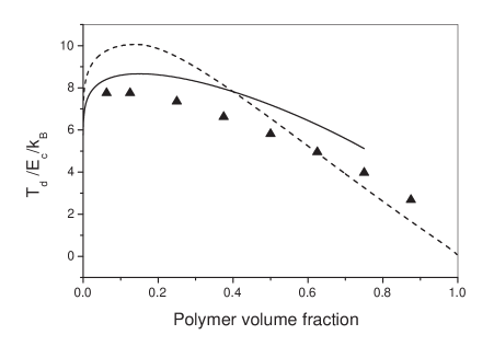
FIG. 3.: Liquid-liquid coexistence curves ($T_{d}$) of the sample system with $E_{p}/E_{c}=0$ and $B/E_{c}=0.25$. The solid line is calculated from the classical Flory-Huggins free-energy expression for polymer solutions, and the dashed line is calculated from the second-order expansion of the mixing free energy in lattice-cluster theory. The triangles are the onsets of liquid-liquid demixing induced by a terraced substrate on cooling. The error bars are smaller than the symbols.

B Polymer crystallization and its interplay with liquid-liquid demixing

When we set $B/E_{c}=0$ and $E_{p}/E_{c}=1$, L-L demixing is preempted by freezing. In fact, an estimate based on mean-field theory (Eqn. 10 below) indicates that, for these parameter values, the freezing temperature of the pure polymer is a factor four higher than the critical demixing temperature. We assume that the onset of crystallization induced by the terraced substrate, yields a good approximation for the equilibrium melting temperature. It is this temperature that we subsequently compare with the corresponding prediction of mean-field theory.

The mean-field expression for the partition function of the disordered polymer solution is given by [8]:

$$Z=(\frac{n}{n_{1}})^{n_{1}}(\frac{n}{n_{2}})^{n_{2}}(\frac{q}{2})^{n_{2}}z_{c}^{(r-2)n_{2}}\text{e}^{(1-r)n_{2}}z_{p}^{(r-1)n_{2}}z_{l}^{rn_{2}},$$ (6)

where
$z_{c}=1+(q-2)\text{exp}(-\frac{E_{c}}{k_{B}T})$,
$z_{p}=\text{exp}[-\frac{q-2}{2}(1-\frac{2(r-1)n_{2}}{qn})\frac{E_{p}}{k_{B}T}]$,
$z_{l}=\text{exp}(-\frac{n_{1}}{n}\frac{(q-2)B}{k_{B}T})$
$n_{1}$ denotes the number of sites occupied by the solvent, $n_{2}$ the number of chains, each having $r$ units, and $n=n_{1}+rn_{2}$. We note that, in the above expression, we have corrected an error in the expression for the partition function given in Ref. 8. The corresponding expression for the free-energy density (i.e. the Helmholtz free energy per lattice site) is

$$\frac{f(\phi)}{k_{B}T} = (1-\phi)\ln(1-\phi)+\frac{\phi}{r}\ln\phi$$ (10)

$$+\phi(-\frac{\ln(qr/2)}{r}-(1-2/r)\ln z_{c}+(1-1/r)$$

$$+(q-2)\frac{B}{k_{B}T}+(1-1/r)\frac{q-2}{2}\frac{E_{p}}{k_{B}T})$$

$$-\phi^{2}\left((q-2)\frac{B}{k_{B}T}+(1-1/r)^{2}\frac{q-2}{q}\frac{E_{p}}{k_{B}T}\right)$$

We assume that the pure polymer crystal is in its fully ordered ground state and that the partition function of this state is equal to one. In a pure polymer system, melting takes place at the point where the free energies of the crystal and the melt cross. For polymer solutions, the freezing curve can be computed by imposing that the chemical potential of the polymers in crystal and solution are equal, i. e. $\mu^{c}-\mu^{0}=\mu^{s}-\mu^{0}$, where $\mu^{0}$ is the chemical potential of polymers in the ground state. As the free energy of the crystal phase is assumed to be equal to zero, the chemical potential of the polymers in that phase is also equal to zero.The chemical potential of the polymers in solution is $\mu^{s}=\partial F^{s}/\partial n_{2}$. Thus by solving the equation $\partial\text{ln}Z^{s}/\partial n_{2}=0$ by iteration, we can obtain the equilibrium melting temperature.

Starting the calculation from Eq. 10, the F-H expression for the mixing free-energy change becomes

$$\frac{\Delta f_{mix}}{k_{B}T} = (1-\phi)\text{ln}(1-\phi)+\frac{\phi}{r}\text{ln}(\phi)$$ (12)

$$+\phi(1-\phi)(q-2)\left(\frac{B}{k_{B}T}+\frac{1}{q}(1-\frac{1}{r})^{2}\frac{E_{p}}{k_{B}T}\right).$$

The binodal L-L curves can be separately estimated without the consideration of L-S curves.

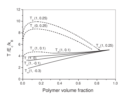
A.

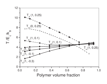
B.

FIG. 4.: Liquid-liquid demixing curves (denoted as $T_{d}$) and liquid-solid transition curves (denoted as $T_{m}$) for the sample system with variable energy parameter settings (denoted as $T(E_{p}/E_{c},B/E_{c})$). (A) Theoretical curves calculated from Eq. 6 with $q_{eff}=q-2$ (Flory-Huggins approach). Note that changing $E_{p}/E_{c}$ from 1 to 0, leads to a 10% decrease in $T_{d}$. In contrast, lowering $B/E_{c}$ by 0.15 reduced $T_{d}$ by more than 50%. An arrow indicates the position of possible triple point; (B) Onsets of phase transitions induced by a terraced substrate on cooling. The error bars are smaller than the symbols, and the segments are drawn to guide the eye.

In Figs. 4A and 4B, we compare the mean-field predictions for the phase diagram with the simulation data. In view of the simplicity of the mean-field theory, the agreement between theory (without adjustable parameters) and the simulation data, is gratifying.

According to Eq. 12, we should expect that a positive value of $E_{p}/E_{c}$ will increase the L-L demixing temperature. This is precisely the behavior observed in Fig. 4, where the L-L demixing curve of the sample system with $B/E_{c}=0.25$ shifts up when the value of $E_{p}/E_{c}$ changes from zero to one. By carefully choosing the parameters, such as $B/E_{c}=0.1$, we can “tune” the relative strength of the tendencies to crystallize and to demix, and observe the intersection of the L-S and L-L curves.

Although a change in the value of $B/E_{c}$ cannot change the freezing temperature of pure polymers, it can change the L-S coexistence curve of polymer solutions. The reason is that a poor solvent favors phase separation (be it L-L or L-S).

However, in the simulations, we observed that the L-S curves cross not only at $\phi=1$ but also at a second point near $\phi=0.73$. This crossing point is not related to the presence of the terraced substrate, as it has also been observed in the absence of such a template.[8] Possibly, this failure of the simple mean-field theory is due to the rather naive way in which it accounts for the effective coordination of monomers. We point out that, in our estimate, we have assumed that the effective coordination number is equal to $q-2$. But, in more sophisticated theoretical descriptions, $q_{eff}$ (as in Eq. 5) is, itself, concentration dependent.

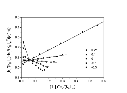
FIG. 5.: Rescaled data in Fig. 4B for the onsets of crystallization induced by a terraced substrate on cooling, according to the formula of Eq. 13 with an approximation of $E_{c}/(k_{B}T_{m}^{0})=0.2$. The solid lines are the results of linear regression of those data points. The meaning of the symbols is the same as those in figure  4B.

Flory has proposed a semi-empirical relationship between the melting point and the concentration of polymers in solutions, [30] as given by

$$\frac{1}{T_{m}}-\frac{1}{T_{m}^{0}}=\frac{k_{B}}{\Delta h_{u}}[1-\phi-\frac{q_{eff}B}{k_{B}T_{m}}(1-\phi)^{2}],$$ (13)

where $T_{m}^{0}$ is the equilibrium melting point of bulk polymers, $\Delta h_{u}$ is the heat of fusion per chain-unit. The predictions of Eq. 13 for the melting-point depression upon dilution have been verified by several experimental measurements at both high and low concentration ends. [31, 32] The linear relationship predicted by Eq. 13 does hold for those simulations where L-L demixing does not occur (see Fig. 5). According to Eq. 13, the values of $-q_{eff}B/\Delta h_{u}$ and $E_{c}/\Delta h_{u}$ can be obtained respectively from the slope and the intercept of the freezing “line”. We found that $-q_{eff}B/\Delta h_{u}$ depends nearly linearly on $B/E_{c}\times E_{c}/\Delta h_{u}$. In addition, $\Delta h_{u}/E_{c}$ varies linearly with $B/E_{c}$. Assuming that both relations are, in fact, linear, we find: $q_{eff}=54.0$ and $\Delta h_{u}=41.0B+13.0E_{c}$ respectively. The latter result implies a microscopic coupling between L-L demixing and polymer crystallization, consistent but not identical with the previous study. [8]

In this paper, we have addressed the equilibrium freezing and demixing curves of lattice polymers. In subsequent work, we shall address the effect of the interplay between demixing and freezing on the kinetics of the phase transformation.

Acknowledgement W.H. acknowledges helpful discussion with Dr. Mark Miller. This work was financially supported by DSM Company. The work of FOM institute is part of the research program of the “Stichting voor Fundamenteel Onderzoek der Materie (FOM)”, which is financially supported by the “Nederlandse organisatie voor Wetenschappelijk Onderzoek (NWO)”.

REFERENCES

- [1] K.H. Meyer, Z. Phys. Chem. (Leipzig) B44, 383(1939).
- [2] P.J. Flory, J. Chem. Phys. 10, 51(1942).
- [3] M.L. Huggins, Ann. N. Y. Acad. Sci. 43, 1(1942).
- [4] R. Koningsveld, L.A. Kleintjens, Macromolecules 4, 637(1971).
- [5] M.G. Bawendi, K.F. Freed, J. Chem. Phys. 88, 2741(1988).
- [6] D. Buta, K.F. Freed, and I. Szleifer J. Chem. Phys. 112, 6040(2000).
- [7] P.J. Flory, Proc. R. Soc. London, Ser. A 234, 60(1956).
- [8] W.-B. Hu, J. Chem. Phys. 113, 3901(2000).
- [9] E.A. Guggenheim, Mixtures (Clarendon, Oxford, 1952).
- [10] P.J. Flory, Principles of Polymer Chemistry (Cornell University Press, Ithaca, NY, 1953).
- [11] I. Prigogine, The Molecular Theory of Solution (Amsterdam, 1957).
- [12] P. R. ten Wolde, D. Frenkel, Science 277, 1975(1997).
- [13] V. Talanquer, D. W. Oxtoby, J. Chem. Phys. 109, 223(1998).
- [14] R.B. Richards, Trans. Faraday Soc. 42, 10(1946).
- [15] L. Aerts, H. Berghmans, and R. Koningsveld, Makromol. Chem. 194, 2697(1993).
- [16] X.W. He, J. Herz, and J.M. Guenet, Macromolecules 20, 2003(1987).
- [17] P. Schaaf, B. Lotz, J. C. Wittmann, Polymer 28, 193(1987).
- [18] H.K. Lee, A.S. Myerson, and K. Levon, Macromolecules 25, 4002(1992) and ref. therein.
- [19] J.M. Guenet, Thermochimica Acta 284, 67(1996).
- [20] H. Berghmans, R. De Cooman, J. De Rudder, and R. Koningsveld Polymer 39, 4621(1998).
- [21] R. Koningsveld, Ph.D. Thesis, University of Leiden, 1967.
- [22] N. Inaba, K. Sato, S. Suzuki, T. Hashimoto, Macromolecules 19,1690(1986).
- [23] W.-B. Hu, J. Chem. Phys. 109, 3686(1998).
- [24] R. G. Larson, L. E. Scriven, H. T. Davis, J. Chem. Phys. 83, 2411(1985).
- [25] I. Camesin, K. Kremer, Macromolecules 21, 2819(1988).
- [26] H. P. Deutsch, K. Binder, J. Chem. Phys. 94, 2294(1991).
- [27] J.-M. Lu, Y.-L. Yang, Sci. China Ser. A 36, 357(1993).
- [28] P.-G. de Gennes, J. Chem. Phys. 55, 571(1971).
- [29] W.-B. Hu, J. Chem. Phys. 115, 4395(2001).
- [30] A. Baumgaertner, J. Chem. Phys. 84, 1905(1986).
- [31] M. Dijkstra, D. Frenkel, Phys. Rev. E 51, 5891(1995).
- [32] H. Weber, W. Paul and K. Binder, Phys. Rev. E 59, 2168(1999).
- [33] Q. Yan, H. Liu, and Y. Hu, Macromolecules 29, 4066(1996).
- [34] B. Quinn, P.D. Gujrati, J. Chem. Phys. 110, 1299(1999).
- [35] K.F. Freed, J. Dudowicz, J. Chem. Phys. 110, 1307(1999).
- [36] P. J. Flory, J. Chem. Phys. 17, 223(1949).
- [37] L. Mandelkern, Crystallization of Polymers (McGraw-Hill Book Co., NY, 1964), p. 38.
- [38] A. Prasad and L. Mandelkern, Macromolecules 22,914(1989).