Currents in System of Noisy Mesoscopic Rings

Abstract

A semi-phenomenological model is proposed to study dynamics and steady-states of magnetic fluxes and currents in mesoscopic rings and cylinders at non-zero temperature. The model is based on a Langevin equation for a flux subject to zero-mean thermal equilibrium Nyquist noise. Quenched randomness, which mimics disorder, is included via the fluctuating parameter method. In the noiseless case, the stability threshold (critical temperature) exists below which selfsustaining currents can run even if the external flux is switched off. It is shown that selfsustaining and persistent currents survive in presence of Nyquist noise and quenched disorder but the stability threshold can be shifted by noise.

PACS number(s): 05.40.-a, 73.23.Ra, 02.50.Ey

1 Introduction

Quantum phenomena manifested at the mesoscopic level have attracted much experimental and theoretical attention. Phase coherence and persistent currents can be mentioned as examples. Persistent currents were predicted as early as 1938 [1] and have been observed experimentally only since 1990 [2]. In the paper we analyze the steady states of magnetic fluxes and currents in a mesoscopic system subject to dissipation and fluctuations [3]. The system consists of a set of concentric one dimensional rings stacked along a certain axis. It is known that a small metallic ring threaded by a magnetic flux displays a persistent current, signifying quantum coherence of electrons (called coherent electrons) and it is a direct manifestation of phase-coherent electron motion and the Aharonov-Bohm effect at the mesoscopic level. Moreover, it has been shown [4] that in such a system selfsustaining currents run even if the external flux is switched off. At temperature $T=0$, the system is in the ground state and only coherent electrons exist. Then the persistent current flows without dissipation. At temperature $T>0$ the amplitude of the persistent current run by coherent electrons decreases and some electrons become ”normal” (i.e. non-coherent). The motion of normal electrons is random and their flow is dissipative. Under some conditions, coherent conduction and normal conduction coexist, resulting in dissipation of a total current. It was confirmed experimentally in [5] that mesoscopic rings connected to a current source presented an Ohmic resistance which was not zero.

We introduce a semi-phenomenological model describing the flux and current in such a system, which takes into account both dissipation and fluctuations. The approach is based on the notion of the two fluid model [6] of normal and coherent electrons formulated as a Langevin equation with a noise term. In the system at temperature $T>0$ there are various sources of noise and fluctuations. There are so-called universal conductance fluctuations [7] that arise from the random quantum interference between many electron paths which contribute to the conductance in the diffusive regime. These fluctuations decay algebraically with temperature and can be neglected at higher temperatures [7]. Inelastic transitions in the ring cause another kind of fluctuations. However, they do not destroy persistent currents but decrease their amplitude [8]. There is also a part of the current noise which is called shot noise [3], the spectral density of which is proportional to mean current. This noise can be reduced by increasing the size of rings [9]. Thermal motion of charge carriers in any conductor is a source of random fluctuations of current which is called Nyquist noise [3]. This thermal equilibrium noise is universal and exists in any conductor, irrespective of the type of conduction and is analogous to noise driving the motion of Brownian particles. Moreover, this noise increases with temperature. Therefore at relatively high temperatures and relatively large rings, universal conductance fluctuations and shot noise can be neglected, and only Nyquist noise can play an important role. This is the case considered in the paper. We assume that coherent and normal electrons coexist [6] and that normal electrons are subjected to Nyquist noise. This noise generates the flux fluctuations which indirectly influence persistent currents run by coherent electrons. Our main goal is to answer the question whether persistent and selfsustaining currents survive in the presence of dissipation and fluctuations. In classical physics dissipation and fluctuations may often be described by introducing random forces into evolution equations. In quantum physics, the inclusion of fluctuations requires more care because quantum systems are described by Hamilton operators and it ensures conservation of energy. In the paper we combine a classical Langevin equation with noise term and with terms of a quantum origin. Our model is minimal in the sense that in two limiting cases it reduces to the well-established models of the quantum persistent current of coherent electrons and the classical Nyquist current of normal electrons. The approach used could be justified in a more elegant way applying the methods of the thermo-field dynamics [10].

The paper is structured as follows. In Sec. II, we describe the model based on the concept of two fluids and introduce the Langevin equation for the magnetic flux, which include Nyquist fluctuations. Its detailed analysis is carried out in Sec. III. In this section, influence of quenched disorder on the system is analyzed as well. Conclusions are made in Sec. IV. Finally, in the Appendix, we present the Nyquist relation from which the intensity of thermal fluctuations is determined.

2 Two fluid model of electronic transport

Persistent currents in conducting structures with topology of the ring are an example of a quantum-interference phenomenon in which the phase coherence of the electron wave function affects equilibrium and transport properties of mesoscopic systems. At zero temperature, $T=0$, the current in a quasi one-dimensional mesoscopic ring threaded by the magnetic field of the Bohm-Aharonov type is paramagnetic [11]

$$I_{even}(\phi)=I_{0}\sum_{n=1}^{\infty}A_{n}\sin\left(\frac{2n\pi\phi}{\phi_{0}}\right)$$ (1)

in the case of an even number of coherent electrons and diamagnetic [11]

$$I_{odd}(\phi)=I_{even}(\phi+\phi_{0}/2)$$ (2)

in the case of an odd number of coherent electrons. Here, $\phi$ is the magnetic flux, $\phi_{0}:=h/e$ is the flux quantum, the amplitudes

$$A_{n}=\frac{2}{\pi n}\cos(nk_{F}l_{x}),$$ (3)

the unit current $I_{0}=heN_{e}/(2l_{x}^{2}m)$, $k_{F}$ is the Fermi momentum, $l_{x}$ is the circumference of the ring and $N_{e}$ is the number of coherent electrons in the ring.

Now, let us consider a collection of rings, individual current channels, which form a cylinder. There are $N_{z}$ channels in direction of the cylinder axis and $N_{r}$ in the direction of the cylinder radius. We assume that the thickness of the cylinder wall is small if compared with the radius. Because of the mutual inductance between rings, the current in one ring induces flux in other rings. In turn, the flux induces a current, and so on. We will analyze the effect of the mutual inductance among the rings. We assume that the rings are not contacted. So, there is no tunneling of electrons among the channels and the charge carriers moving in the different rings are independent. It has been shown in [12] that the effective interaction between the ring currents, when taken in the selfconsistent mean field approximation, results in the magnetic flux $\phi=LI_{tot}$ felt by all electrons, where $L$ is the cylinder inductance and $I_{tot}$ is the total current in a cylinder. For a cylinder of the radius $r$ and the height $l_{z}$ the inductance is [13]

$$L=\mu_{0}\frac{\pi r^{2}}{l_{z}},$$ (4)

where $\mu_{0}$ is the permeability of the free space. At temperature $T>0$, the current $I_{coh}(\phi,T)$ of the coherent electrons in a set of $N=N_{r}\times N_{z}$ current channels forming the cylinder is either [4]

$$I_{coh}(\phi,T)=I_{even}(\phi,T)\\ =NI_{0}\sum_{n=1}^{\infty}A_{n}(T)\sin\left(\frac{2n\pi\phi}{\phi_{0}}\right)$$

for an even number of coherent electrons in each single channel or

$$I_{coh}(\phi,T)=I_{odd}(\phi,T)=I_{even}(\phi+\phi_{0}/2,T)$$ (5)

for an odd number of coherent electrons. The amplitude

$$A_{n}(T)=\frac{4T}{\pi T^{*}}\frac{\exp(-nT/T^{*})}{1-\exp(-2nT/T^{*})}\cos(nk_{F}l_{x}).$$ (6)

The characteristic temperature $T^{*}$ is given by the relation $k_{B}T^{*}=\Delta_{F}/2\pi^{2}$, where $k_{B}$ is the Boltzmann constant and $\Delta_{F}$ is the energy gap at the Fermi surface. For temperatures $T<T^{*}$ the coherent current flows in such a cylinder without dissipation but its amplitude (6) is reduced [11]. On the other hand, at temperature $T>0$, normal electrons occur and their flow is dissipative. The motion of normal electrons is random, like the motion of electrons in a normal conductor and it generates random currents.

The current coming from the normal electrons can be induced by e.g. the change of the magnetic flux $\phi$. According to the Lenz’s rule and the Ohm’s law one gets [14]

$$RI_{nor}(\phi)=-\frac{d\phi}{dt},$$ (7)

where $R$ is the effective resistance of the system [8].

At temperature $T>0$, coherent and normal electrons can coexist resulting in dissipation of the total current $I_{tot}$ which, in the absence of fluctuations, is a sum of the persistent and normal currents,

$$I_{tot}(\phi,T)=I_{coh}(\phi,T)+I_{nor}(\phi).$$ (8)

The magnetic flux is related to the total current via the expression

$$\phi=\phi_{ext}+LI_{tot}(\phi,T),$$ (9)

i.e. it is a sum of the external flux $\phi_{ext}$ and the flux coming from the currents.

Combining (8), (7) and (9) yields the equation

$$\frac{1}{R}\frac{d\phi}{dt}=-\frac{1}{L}(\phi-\phi_{ext})+I_{coh}(\phi,T).$$ (10)

It is known that the current-flux characteristics for the coherent electrons is extraordinary sensitive to a change of parity of the coherent carriers number [11]. In order to take into account the possible difference of parity in the rings we consider the current of coherent electrons as the average $I^{av}_{coh}(\phi,T)=pI_{even}(\phi,T)+(1-p)I_{odd}(\phi,T)$, where $p\in[0,1]$ is the probability of the even number of coherent electrons in a given channel.

The term describing current fluctuations should also be included in the evolution equation (10). Within our model, the only source of fluctuations is the equilibrium Nyquist normal current noise generated by the resistance $R$. The correlation function of this source of fluctuations is assumed to be given by the Nyquist relation. It follows from the Appendix that Eq. (10) should be modified to the following form

$$\frac{1}{R}\frac{d\phi}{dt}=-\frac{1}{L}(\phi-\phi_{ext})+I_{coh}^{av}(\phi,T)+\sqrt{\frac{2k_{B}T}{R}}\;\Gamma(t),$$ (11)

where $\Gamma(t)$ is Gaussian white noise (see the Appendix). This equation takes the form of a classical Langevin equation and is our basic evolution equation.

Let us introduce dimensionless variables. In the Langevin equation (11), the basic quantity is the magnetic flux $\phi=\phi(t)$. The natural unit of the flux is the flux quantum $\phi_{0}=h/e$. Accordingly, the flux is scaled as $x=\phi/\phi_{0}$. To identify the characteristic time $\tau_{0}$, let us consider a particular case of (11), namely, when the persistent current and the external flux are zero. Then

$$\frac{d\phi}{dt}=-\frac{R}{L}\phi+\sqrt{2Rk_{B}T}\;\Gamma(t).$$ (12)

From this equation it follows that the mean value

$$\langle\phi(t)\rangle=\langle\phi(0)\rangle\,\exp(-t/\tau_{0}),$$ (13)

where

$$\tau_{0}=L/R$$ (14)

is the relaxation time of the averaged normal current. Therefore time is scaled as ${\tilde{t}}=t/\tau_{0}$. In this case, Eq. (11) can be transformed into its dimensionless form

$$\dot{x}=-V^{\prime}(x)+\sqrt{2D}\;\widetilde{\Gamma}({\tilde{t}}),$$ (15)

where the dot denotes a derivative with respect to the rescaled time ${\tilde{t}}$ and the prime denotes a derivative with respect to $x$. The generalized potential

$$V(x)=V(x,\lambda,i_{0},p,T)=\frac{1}{2}x^{2}-\lambda x-i_{0}F(x,p,T),$$ (16)

where $\lambda=\phi_{ext}/\phi_{0}$ is the rescaled external flux. The prefactor $i_{0}=NLI_{0}/\phi_{0}$ is a coupling constant characterizing the interaction between ring currents (it is the rescaled amplitude of the flux created by the current - it leads to selfsustaining currents). The function

$$F(x)=F(x,p,T)=\int f(x,p,T)dx$$ (17)

characterizes the coherent electrons and

$$f(x,p,T)=pf_{even}(x,T)+(1-p)f_{odd}(x,T),$$ (18)

where

$$f_{even}(x,T)=\sum_{n=1}^{\infty}A_{n}(T)\sin(2n\pi x)$$ (19)

and

$$f_{odd}(x,T)=f_{even}(x+1/2,T).$$ (20)

The dimensionless intensity $D$ of rescaled Gaussian white noise $\widetilde{\Gamma}({\tilde{t}})\equiv\sqrt{\tau_{0}}\;\Gamma(\tau_{0}{\tilde{t}})$ is a ratio of thermal energy to the elementary energy stored up in the inductance,

$$D=\frac{1}{2}k_{B}T/\epsilon_{0},\qquad\epsilon_{0}:=\frac{\phi_{0}^{2}}{2L}.$$ (21)

The rescaled Gaussian white noise $\widetilde{\Gamma}({\tilde{t}})$ has the same moments as in (36). Let us notice that the resistance $R$ does not occur explicitly in the rescaled equation (15).

Let us evaluate the order of magnitude of the parameters appearing in our equations. The rescaled coupling constant

$$i_{0}=\frac{\mu_{0}e^{2}N}{8\pi m_{e}}\frac{N_{e}}{l_{z}}.$$ (22)

We assume that the cylinder has the radius $r=3\cdot 10^{4}\mathring{A}$ and the height $l_{z}=100\mathring{A}$. It consists of a set of $N\sim 50$ current channels [15] in a wall of width much smaller than the radius. If the number of electrons in each channel is $N_{e}\sim 2\cdot 10^{5}$ then $i_{0}\sim 1$. The energy gap at the Fermi surface $\Delta_{F}=\hbar^{2}N_{e}/(2m_{e}r^{2})$ gives the rescaled noise amplitude

$$\frac{k_{B}T^{\ast}}{2\epsilon_{0}}=\frac{\mu_{0}e^{2}}{16\pi^{3}m_{e}}\frac{N_{e}}{l_{z}}.$$ (23)

For the above values of parameters the diffusion coefficient $D\sim 0.001T/T^{\ast}$. Below, unless stated otherwise, the parameter are fixed so that $i_{0}=1$ and $D=0.001T/T^{\ast}$.

3 Analysis

In this section the properties of system described by Eq. (15) are analyzed. We consider in details three special cases. In the deterministic - noiseless - case, we neglect the influence of Nyquist noise. It is a justified approximation for very small intensity of noise. In the second case, we include Nyquist noise, i.e. we analyze the full version of (15). In the third case, we extend the model assuming that the coupling parameter $i_{0}$ is a random variable. It can mimic uncorrelated, quenched disorder of the rings.

As follows from (9), the current $I_{tot}$ is linearly related to the magnetic flux $\phi$ (or the rescaled flux $x$). In a consequence, the properties and behavior of the current are identical to the properties and behavior of the magnetic flux. Therefore, below we discuss mostly the dependence of the magnetic flux on the parameters of the model.

3.1 Noiseless case

First, let us consider the deterministic case of the Langevin stochastic equation (15) formally neglecting the Nyquist noise term $\tilde{\Gamma}({\tilde{t}})$, i.e.,

$$\dot{x}=-V^{\prime}(x).$$ (24)

The stationary solutions $x_{s}$ of (24), for which $\dot{x}_{s}=0$, correspond to extrema of the generalized potential (16),

$$V^{\prime}(x_{s})=x_{s}-\lambda-i_{0}f(x_{s},p,T)=0.$$ (25)

The solutions $x_{s}$ of the gradient differential equation (24) are stable provided they correspond to a minimum of the generalized potential (16) and they are unstable in the case of a maximum [16]. In the following we investigate properties of solutions $x_{s}$ with respect to four independent parameters: the temperature $T$, the coupling constant $i_{0}$ which characterizes the mean-field interaction between rings, the probability $p$ of the occurrence of the channel with an even number of coherent electrons and the external flux $\lambda$.

3.1.1 $T$ and $i_{0}$-dependence

The dependence of the potential (16) on the temperature for $\lambda=0$, $i_{0}=1$ and the probability $p=1/2$ is shown in Fig. 1.

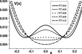
Figure 1: Dimensionless generalized potential $V(x)$ given by Eq. (17) is shown as a function of the dimensionless magnetic flux $x$ for several values of the scaled temperature $T/T^{*}$. The scaled amplitude $i_{0}=1$ and scaled external magnetic flux $\lambda=0$.

In high temperatures, only one stable solution, corresponding to zero stationary flux $x_{s}=0$ and zero current, exists. If temperature decreases, a bifurcation occurs - the potential becomes bistable and two non-zero symmetric minima appear at $x_{s}=\pm x_{m}$. They correspond to two stable stationary solutions. Physically, it means that below some critical temperature $T_{c}$ the spontaneous flux [17] appears and non-zero stationary current flows in the system. This critical temperature $T_{c}$ is defined by the condition that $V^{\prime\prime}(x_{s}=0)=0$. The corresponding diagram is shown in Fig. 2.

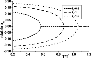
Figure 2: Bifurcation of the stable stationary magnetic flux $x_{s}$ determined by Eq. (26) is depicted vs temperature $T/T^{*}$ for several values of $i_{0}$ and fixed external flux $\lambda=0$.

The phenomenon is analogous to the continuous phase transition in macroscopic systems, and appears here as a result of the interaction of ring currents. The central maximum $x_{s}=x_{M}=0$, corresponds to the unstable stationary solution of (24).

More generally, one can notice that the stationary solutions occur where the linear part $x-\lambda$ of (25) is equal to its periodic part $i_{0}f(x,p,T)$. In the limit of $i_{0}\rightarrow 0$ (very small, or no interaction of ring currents), regardless $T$, the only stationary solution of (25) is the external flux $x_{s}=\lambda$. For intermediate $i_{0}$ (typical interaction of mesoscopic rings) two stable non-zero stationary states can exist below $T_{c}$ and this number of solutions is preserved in the limit $T\rightarrow 0$. As one can infer from (16)-(20), decreasing temperature enhances the periodic part of (25) but only to a maximal value defined by $T\rightarrow 0$. Further enhancement of the periodic part is possible only by increasing the coupling constant $i_{0}$. As a result of that, the critical temperature $T_{c}$ increases with $i_{0}$. Therefore, if $i_{0}$ is sufficiently large (very strong interaction of rings), even more stationary states can occur. The number of stationary states below $T_{c}$ and for $p=1/2$ can, in general, be equal to $4k-1,$ $(k=1,2...)$ but only $2k$ of them of stable states. Lowering the temperature below $T_{c}$ results then in a cascade of bifurcations. The first bifurcation takes place at $T=T_{c}$. With further lowering the temperature at $T=T_{c_{1}}<T_{c}$ two additional pairs of stationary solutions appear and so on. There is one metastable and one unstable solution in every pair. The metastable solutions correspond to the so called flux trapped in the cylinder. Notice that in the limit $T\rightarrow 0$ and typical $i_{0}>0$ there are always spontaneous flux solutions whereas the flux trapped solutions can be obtained only for sufficiently large $i_{0}$.

3.1.2 The $p$-dependence

In the following part of this section the temperature is set below $T_{c}$. If the probability $p=1$ we have an even number of coherent electrons and paramagnetic current in each channel. The potential possesses two minima corresponding to spontaneous fluxes. Decreasing $p$, the probability $1-p$ of finding odd channels with diamagnetic currents increases and the spontaneous flux solutions $x_{s}$ decrease to coalesce finally into a single absolutely stable solution at $x_{s}=0$. The ratio $p$ at which the coalescence occurs decreases with decreasing temperature. Now, for sufficiently large $i_{0}$, five stationary states exist. Note that apart from the stable fluxless solution $x_{s}=0$ there are two metastable solutions at $\frac{1}{2}<|x_{s}|<1$ and two unstable solutions. The metastable solutions correspond to the flux trapped in the cylinder. In realistic devices they are hardly accessible due to the value of the necessary parameters. Further the discussion is limited to the case when $p=1/2$.

3.1.3 The $\lambda$-dependence

The dependence of the stationary solutions $x_{s}$ on the external flux $\lambda$ is shown in Fig. 3.

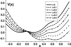
Figure 3: Generalized potential (17) for several values of the external flux $\lambda$, fixed $i_{0}=1$ and $T/T^{*}=0.2$.

There are three different types of the generalized potential. First is a symmetric double well potential which appears for $\lambda=k/2$ with integral $k$. The stable solutions $x_{s}$ are then always around the external flux $0<|x_{s}-\lambda|<\frac{1}{2}$. For the values of $\lambda$ close but not equal to $k/2$ the solutions remain in that range but the double-well potential becomes asymmetric - one of the stable solutions becomes metastable. For the values of external flux far from half integer values $k/2$ one obtains the potential with only a single stable solution. All the mentioned types of potentials are accessible for $0\leq\lambda<1/2$ indicating a kind of the ’structural periodicity’ with respect to the external flux.

An interesting feature of the $x-\lambda$ characteristic is the occurrence of the hysteresis loop (Fig.4).

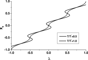
Figure 4: The stationary magnetic flux $x_{s}$ determined by Eq.(26) vs external flux $\lambda$ and two distinct temperatures. For $T/T^{*}=0.5$ the part of the graph with the negative slope corresponds to unstable $x_{s}$. The dependence of $x_{s}$ on $\lambda$ is in this case hysteretic. The amplitude $i_{0}=1$.

With increasing $\lambda,$at its certain value, the system undergoes discontinuous jump of $x$. Decreasing then the value of $\lambda$, the opposite jump of $x$ occurs at lower $\lambda$ producing a hysteresis loop. It is a hallmark of the first order phase transition. The transition can occur only below the critical temperature $T_{c}$. Due to the ’structural periodicity’ the hysteresis loop is repeated with the period $\lambda=1/2$ what results in the formation of a family of loops.

3.2 Model with Nyquist noise

Noise and fluctuations are ubiquitous in real systems and idealization of the noiseless systems is sometimes not justified. In the following, we will focus on the system (15) subjected to Nyquist noise. From the mathematical point of view, the Langevin equation (15) defines a Markov diffusion process. Its probability density $p(x,{\tilde{t}})$ obeys the Fokker-Planck equation in the form

$$\frac{\partial}{\partial{\tilde{t}}}p(x,{\tilde{t}})=\frac{\partial}{\partial x}V^{\prime}(x)p(x,{\tilde{t}})+D\,\frac{\partial^{2}}{\partial x^{2}}p(x,{\tilde{t}})$$ (26)

with the natural boundary condition $\lim_{|x|\rightarrow\infty}p(x,{\tilde{t}})=0$. The stationary solution $p_{s}(x)$ is asymptotically stable [19] and takes the form

$$p_{s}(x)=N_{0}\mbox{e}^{-V(x)/D}$$ (27)

with a normalization constant

$$N_{0}^{-1}=\int_{-\infty}^{\infty}\mbox{e}^{-V(x)/D}\;dx.$$ (28)

Let us first consider the case of absence of the external flux, $\lambda=0$. If in the noiseless case the system possesses only one stationary solution $x_{s}=0$, the probability density (27) has maximum at $x=0$ and the mean value of the flux $\langle x\rangle=0$. If in the noiseless case the system possesses three stationary states, the probability density (27) has three extremal points: two symmetric maxima which correspond to the spontaneous fluxes and one minimum at $x=0$ which corresponds to the unstable stationary state (see Fig. 1). Because the potential is reflection-symmetric, $V(x)=V(-x)$, the mean value of any odd function of the flux is zero. In particular, the mean value of the flux $\langle x\rangle=0$ and the mean value of the current is zero as well. From this point of view, properties of stationary states are trivial and non-zero fluxes and currents are impossible. However, in some situations the statistical moments are not good characteristics of the system because much information is lost when an integration is performed calculating the statistical moments [20]. The relevant quantity is a stationary probability distribution which contains much more information about the system. Is any reasonable method to determine the critical value of temperature $T_{c}$ in this case? One possibility is to define the phase transition in the following way [20, 21]: the phase transition point is a value of the relevant parameter $\gamma$ of the system at which the profile of the stationary distribution function changes drastically (e.g. if a number of maxima of the distribution function changes) or if a certain most probable point $x_{0}$ begins to change to an unstable state. In some cases, it is indeed a good ’order parameter’ of the system. For example, from the measurements of the laser experiment (see e.g. [22]), one can obtain the stationary probability distribution of the laser intensity and one can observe a phase transition according to the above definition. In the case considered here, for sufficiently low temperatures, thermal fluctuations are small and one expects the experimental results to be accumulated around the most probable values of the stationary probability distribution. It follows from (27) that the most probable values of the flux corresponds exactly to the stationary states (25) of the system (24). In this sense, the properties of the system are the same as discussed in the previous subsection. We want to emphasize that it is correct for low temperatures because then the residence time in a stable state is long. For higher temperature $T$, thermal fluctuations become larger. In turn, fluctuations of the magnetic flux around the most probable value become larger and larger and the residence time in a stable state becomes shorter. One can guess that the spontaneous current should vanish at temperature $T_{0}$ which is lower than the critical temperature $T_{c}$ in the noiseless case. This is because of influence of Nyquist fluctuations. The argumentation is the following. If the potential is multistable then one can introduce characteristic time scales of the system. The first characteristic time $\tau_{d}=1/V^{\prime\prime}(x_{s})$ describes decay within the attractor $x_{s}=\pm x_{m}$ of the potential $V(x)$. The second characteristic time is the escape time $\tau_{e}$ from the well around $\pm x_{m}$. This time is related to the mean first passage time from the minimum of the potential to the maximum. If these time scales are well separated, i.e. if $\tau_{e}>>\tau_{d}$ then the description based on the most probable value seems to be correct. Otherwise, this description fails and we should characterize the system by averaged values of relevant variables. The exact formula for the escape time $\tau_{e}$ is known [23] but is not reproduced here. We have calculated $\tau_{e}$ for the transition from the left minimum of the potential (16) assuming that the left boundary at $-\infty$ is reflecting and the right boundary at the maximum $x_{M}$ of the potential is absorbing.

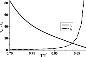
Figure 5: Plot of the characteristic escape time $\tau_{e}$ and decay time $\tau_{d}$ as a function of temperature $T/T^{*}$ for $i_{0}=1$, $\lambda=0$ and the strength of Nyquist noise $D=0.001T/T^{*}$.

In Fig. 5 we show the dependence of two characteristic times $\tau_{e}$ and $\tau_{d}$ upon the rescaled temperature $T/T^{*}$. The escape time $\tau_{e}$ is a monotonically decreasing function of temperature while the decay time $\tau_{d}$ monotonically increases with temperature. In the noiseless case, for values of parameters chosen in Fig. 5 and from Eq.(16) we estimated the critical temperature $T_{c}\approx 0.88T^{*}$. One can observe that roughly for temperatures $T<0.8T^{*}$, the characteristic time $\tau_{d}$ is more than one order of magnitude less than $\tau_{e}$. Both time scales are well separated and selfsustaining currents are long-living states. In this sense, they are not destroyed by Nyquist noise.

Temperature $T$ enters into the Langevin equation (15) in two-fold: it contributes to the intensity $D=k_{B}T/\epsilon_{0}$ of Nyquist noise and to the effective interaction between the rings via the potential (16) describing coherent electrons current. The influence of temperature on the properties of equilibrium distribution is plotted in Fig. 6.

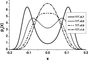
Figure 6: Probability density (28) for selected values of temperature, fixed $i_{0}=1$, $\lambda=0$ and $D=0.001T/T^{*}$.

As stated before the position of the most probably values correspond to stable stationary states. The statistically averaged current vanishes since $\langle x\rangle=0$. The stationary flux variance or mean-squared deviation $\sigma=\langle x^{2}\rangle-\langle x\rangle^{2}=\langle x^{2}\rangle$ is a non-monotonic function of temperature (Fig. 7): For $T=0$ the variance $\sigma=x_{s}^{2}$, where $x_{s}$ is a stationary solution of (24). As the temperature increases, $\sigma$ diminishes attaining a minimal value at some temperature $T_{1}$. The temperature $T_{1}$ seems to be always larger than $T_{c}$ what is confirmed in the numerical studies.

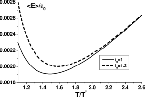
Figure 7: Averaged magnetic energy $\langle E\rangle/\epsilon_{0}$ given by Eq.(31) vs scaled temperature for two values of $i_{0}$, fixed $\lambda=0$ and $D=0.001T/T^{*}$.

A further increase of temperature leads to an increase of the variance. In the high temperature limit, the dependence is linear as for the Gaussian distribution. Indeed, below the critical temperature, the distribution (27) possessing two peaks is clearly non-Gaussian. However, for higher temperatures the probability density is one-peaked. For this case, the kurtosis

$$Kurt=\frac{\langle x^{4}\rangle}{3\langle x^{2}\rangle^{2}}-1$$ (29)

measures the relative flatness of the distribution (27) to the Gaussian distribution. The kurtosis is negative and it means that the distribution (27) is flat. It approaches zero in the high temperature limit and then the distribution (27) approaches the Gaussian distribution.

The behavior of the second moment $\langle x^{2}\rangle$ has a simple explanation in terms of the average energy stored in the magnetic field, i.e

$$\langle E\rangle=\langle\phi^{2}\rangle/2L=\epsilon_{0}\langle x^{2}\rangle,$$ (30)

where $\epsilon_{0}$ is given in (21). For low temperatures, fluctuations are small and the main contribution to the energy comes from the deterministic part $\phi^{2}/2L$. Because the magnetic flux $\phi$ decreases as temperature increases (cf. Fig. 2), hence $\langle E\rangle$ decreases as well. On the other hand, for high temperature the stationary probability density approaches the Gaussian distribution and in consequence the main contribution to the average magnetic energy comes from thermal energy, $\langle E\rangle\propto kT$ which obviously increases when $T$ grows. The competition between these two mechanisms leads to the minimal value of $\langle E\rangle$ for a certain value of temperature $T_{1}$.

The influence of the external field on the properties of the stationary density (27) may be deduced from Fig. 3. Finally, let us consider the limit of a very weak coupling between the ring currents corresponding to a very small value of $i_{0}$. The selfsustaining stable solutions are non accessible. The solutions of Eq.(24) correspond then to the persistent currents driven by the external field. The stationary density forms a family of one peak curves with the most probable values given by $\lambda$. We conclude that even in the weak coupling limit the presence of Nyquist noise does not destroy the persistent currents.

3.3 Model with quenched disorder

There are several sources of disorder which can be described as quenched fluctuations. The first one is caused by impurities distributed randomly in the cylinder. The presence of impurities leads to modification of the coherent current amplitude [15]. Another source of disorder is of a geometrical origin. The radius of rings being not exactly of the same value may change randomly from one ring to the other. Also the number $N_{r}$ of current channels in the direction of the cylinder radius can be, in general, different in every point of vertical axis of the cylinder. These sources of disorder can be included into our model assuming that deviations of the coherent current amplitude from the average are small and

$$i_{0}=j_{0}+\epsilon\xi,$$ (31)

where $j_{0}$ is an averaged value of the amplitude $i_{0}$, $\epsilon$ characterizes intensity of quenched fluctuations, $\xi$ is a zero-mean random variable of values in the interval $[-1,1]$ and of the probability density $P_{\xi}(z)$.

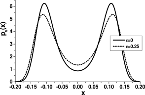
Figure 8: Probability density (33) for the system with ($\varepsilon=0.25$) and without ($\varepsilon=0$) quenched disorder for $T/T^{*}=0.7$, $j_{0}=1$, $\lambda=0$ and $D=0.001T/T^{*}$ .

The stationary probability density $p_{s}(x)$ of the flux is now expressed as

$$p_{s}(x)=\int_{-1}^{1}p(x|z)P_{\xi}(z)\;dz,$$ (32)

where the conditional probability distribution

$$p(x|z)=C_{0}(z)\;\mbox{e}^{-[V(x)-\epsilon zF(x)]/D}$$ (33)

has the same form as (27) with the replacement $i_{0}=j_{0}+\epsilon z$ in the potential (16). Now, the normalization constant depends on $z$, namely,

$$C_{0}^{-1}(z)=\int_{-\infty}^{\infty}\mbox{e}^{-[V(x)-\epsilon zF(x)]/D}\;dx.$$ (34)

In Fig. 8 we show the distribution (32) for $p=1/2$, $\lambda=0$ and the uniform probability distribution $P_{\xi}(z)$. The observed shift of the most probable value of the flux is rather small and can be interpreted as an increase of the magnitude of the selfsustaining current. The magnitude of peaks does not change significantly as well. One observes that both the depth of the minimum and the height of the maxima decrease. One concludes that the quenched disorder does not drastically change the properties of the flux with only one exception. The probability density in or near the critical temperature $T_{c}$ may change qualitatively from one peak to two peaks. In the critical region the quenched disorder lowers the critical temperature $T_{c}$.

4 Summary

Persistent and selfsustaining currents are beautiful manifestation of quantum coherence in mesoscopic systems. The natural question is how do they behave in the presence of dissipation and fluctuations. Assuming the two fluid model for mesoscopic system we have investigated the influence of Nyquist noise and quenched disorder on these currents. Our discussion is limited to stationary states of the magnetic flux and current although the proposed model of the flux dynamics can be, in principle, applied to study time dependent problems.

The deterministic system, obtained as a formal noiseless limit, exhibits critical behavior such as bifurcations (phase transitions) and hysteresis. There is a critical temperature $T_{c}$ below which non-zero selfsustaining currents flow. For the noisy system, we have investigated the properties of the flux probability. We have compared the statistical properties of the stationary probability density with the deterministic case. Maxima of the stationary probability density correspond exactly to the deterministic stable solutions while the local minima to the unstable solutions. In the presence of randomness, there is a problem of defining the critical temperature. We have presented three points of view which are based on the mean value of the flux (no phase transitions), on the maxima of the probability density (the same critical properties as in the deterministic case) and on the comparison of two characteristic times (the critical temperature lower than in the deterministic case).

The interesting finding is that the mean magnetic energy as a function of the temperature is not monotonic - for low temperatures it is decreasing while for high temperature it is an increasing function. The minimum is not at the critical temperature $T_{c}$ but at temperature $T_{1}>T_{c}$. Moreover, we have included quenched disorder and concluded that the system is stable with respect to such a perturbation, although the most probable values of the stationary probability density increase. It might be interpreted as an enhancement of the current under the influence of the quenched disorder. Therefore it serves as one more example of the constructive role of fluctuations. The possibility of the noise-induced current in mesoscopic rings has been considered in [24, 25]. The presented approach can be applied not only to analysis of currents in mesoscopic cylinders but also in superconducting rings. There is also another class of mesoscopic systems where our model can be applied - carbon nanotubes. The possibility of persistent currents in carbon nanotubes has been investigated in [26].

The general conclusion is that persistent and selfsustaining currents survive in the presence of the above mentioned fluctuations. However, if the intensity of Nyquist noise or quenched disorder is sufficiently strong they lead to the lowering of the temperature below which the system is in the ordered state. For smaller noise intensity the influence of fluctuations on coherent currents is very small and it is very favorable for the experimental observations of persistent and selfsustaining currents.

5 Appendix

For the paper to be self-contained, we remind one of the form of the fluctuation-dissipation theorem and the Nyquist relation exploited in our basic Eq. (11). The Brownian motion of a particle of mass $m$ in a fluid of temperature $T$ is described by a Langevin equation [27]. According to the fluctuation-dissipation theorem [27], its form for the velocity $v=v(t)$ reads

$$m\dot{v}+\gamma v=\sqrt{2\gamma k_{B}T}\;\Gamma(t),$$ (35)

where a dot denotes a derivative with respect to time, $\gamma$ is the friction coefficient, $k_{B}$ is the Boltzmann constant and $\Gamma(t)$ is the zero-mean and Dirac $\delta$-correlated Gaussian stochastic process (white noise),

$$\langle\Gamma(t)\rangle=0,\quad\langle\Gamma(t)\Gamma(s)\rangle=\delta(t-s).$$ (36)

Mutatis mutandis, the Langevin equation for the current $I=I(t)$ in the $RL$ circuit takes the form [23]

$$L\dot{I}+RI=\sqrt{2Rk_{B}T}\;\Gamma(t).$$ (37)

It is one of the form of the Nyquist relation. In the case when

$$\phi=LI$$ (38)

it can be rewritten as

$${\frac{1}{R}}\frac{d\phi}{dt}+\frac{1}{L}\phi=\sqrt{\frac{2k_{B}T}{R}}\Gamma(t)$$ (39)

which justifies the prefactor of the noise term in Eq. (11).

References

- [1] F. Hund, Ann. Phys. (Leipzig) 32, 102 (1938); M. Buttiker, Y. Imry, R. Landauer, Phys. Lett. 96A, 365 (1983).
- [2] L. P. Levy, G. Dolan, J. Dunsmuir and H. Bouchiat, Phys. Rev. Lett. 64, 2074 (1990).
- [3] Sh. Kogan, Electronic Noise and Fluctuations in Solids (Cambridge University Press, Cambridge, 1996).
- [4] M. Szopa, E. Zipper, Solid. State. Comm. 77, 739 (1991); D.Wohlleben et al. Mod. Phys. Lett. B 6, 1481 (1992).
- [5] H. Bouchiat, in Mesoscopic Quantum Physics, eds. E. Akkermans et al. (North-Holland, Amsterdam, 1995).
- [6] E. Zipper, M. Lisowski, Eur. Phys. J. B 1, 215 (1998).
- [7] T. Dittrich, P. Hänggi, G.-L. Ingold, B. Kramer, G. Schön, W. Zwerger, Quantum Transport and Dissipation (Wiley-VCH, Weinheim, 1998).
- [8] L. Landauer and M. Buttiker, Phys. Rev. Lett. 54, 2049 (1985).
- [9] Y. Imry, Introduction to Mesoscopic Physics (Oxford University Press, New York, 1997).
- [10] H. Umezawa, H. Matsumoto and M. Tachiki, Thermo Field Dynamics and Condensed States (North-Holland, Amsterdam, 1982).
- [11] H.F. Cheung, Y. Gefen, E.K. Riedel, W.H. Shih, Rhys. Rev. B 37,6050 (1988).
- [12] M. Lisowski, E. Zipper, M. Stebelski, Phys. Rev. B 59, 8305 (1999).
- [13] F. Bloch, Phys. Rev. 137, 787 (1965).
- [14] J.D. Jackson, Classical Electrodynamics (PWN, Warszawa, 1987).
- [15] E.K. Riedel, H. Cheung, Physica Scripta T 25, 357 (1989).
- [16] J. Hale, H. Koçak, Dynamics and Bifurcations (Springer, New York, 1991).
- [17] M. Szopa, E. Zipper, Int. J. Mod.Phys. B 9, 161 (1995).
- [18] M. Szopa, D. Wohlleben, E. Zipper, Phys. Lett. A 160, 271 (1991).
- [19] A. Lasota, M.C. Mackey, Probabilistic Properties of Deterministic Systems (Cambridge University Press, Cambridge, 1985).
- [20] W. Hosthemke and R. Lefever, Noise-Induced Transitions (Springer, Berlin, 1984).
- [21] M. Suzuki, Adv. Chem. Phys. 46, 195 (1981).
- [22] P. Lett, E. C. Gage, and T. H. Chyba, Phys. Rev. A 35, 746 (1987).
- [23] C.W. Gardiner, Handbook of Stochastic Methods for Physics, Chemistry and the Natural Sciences (Springer, Berlin, 1998).
- [24] V.E. Kravtsov, B.L. Altshuler, Phys. Rev. Lett. 84, 3394 (2000).
- [25] P. Mohanty, Ann. Phys. 8, 549 (1999).
- [26] M. Szopa, M. Margańska, E. Zipper, Phys. Lett. A, in press.
- [27] H. Risken, The Fokker-Planck Equation (Springer, Berlin, 1984).