Frequency and Phase Synchronization in Stochastic Systems

Abstract

The phenomenon of frequency and phase synchronization in stochastic systems requires a revision of concepts originally phrased in the context of purely deterministic systems. Various definitions of an instantaneous phase are presented and compared with each other with special attention payed to their robustness with respect to noise. We review the results of an analytic approach describing noise-induced phase synchronization in a thermal two-state system. In this context exact expressions for the mean frequency and the phase diffusivity are obtained that together determine the average length of locking episodes. A recently proposed method to quantify frequency synchronization in noisy potential systems is presented and exemplified by applying it to the periodically driven noisy harmonic oscillator. Since this method is based on a threshold crossing rate pioneered by S.O. Rice the related phase velocity is termed Rice frequency. Finally, we discuss the relation between the phenomenon of stochastic resonance and noise-enhanced phase coherence by applying the developed concepts to the periodically driven bistable Kramers oscillator.

Studying synchronization phenomena in stochastic systems necessitates a revision of concepts originally developed for deterministic dynamics. This statement becomes obvious when considering the famous phase-locking effect arnold ; Strato67 : unbounded fluctuations that occur, for instance, in Gaussian noise will always prevent the existence of a strict bound for the asymptotic phase difference of two systems. Nevertheless, a reformulation of the synchronization phenomenon in the presence of noise is possible by quantifying the average duration $\langle T_{\rm lock}\rangle$ of locking epochs that are disrupted by phase slips. In case that $\langle T_{\rm lock}\rangle\gg T_{0}$, where $T_{0}$ is some characteristic time of the dynamics, e.g. the period of an external drive or the inverse of some intrinsic natural frequency, it is justified to speak about effective phase synchronization.

I Introduction

From the conceptual point of view different degrees of synchronization can be distinguished: complete synchronization cs , generalized synchronization gs , lag synchronization ls , phase synchronization ps1 ; ps2 , and burst (or train) synchronization bs . In the following, we focus our attention on phase synchronization in stochastic systems that has attracted recent interest for the following reason: in many practical applications the dynamics of a system, though not perfectly periodic, can still be understood as the manifestation of a stochastically modulated limit cycle book ; biophys . As examples, we mention neuronal activity neurons , the cardiorespiratory system cardresp , or population dynamics popdynamics .

Given a data set or some model dynamics there exists a variety of methods to define an instantaneous phase $\phi(t)$ of a signal or a dynamics. For a clear cut separation of deterministic and noise-induced effects it is essential to assess the robustness of each of these different phase definitions with respect to noise. Section II is devoted to this issue. Since we do not distinguish between dynamical and measurement noise dynmeasnoise our treatment is also tied to the question how synchronization can be detected within any realistic experimental data.

The synchronization properties of a noisy system can be classified in a hierarchical manner: stochastic phase locking always implies frequency locking while the converse is not true in general. On the other hand, small phase diffusivity is necessary but not sufficient for phase synchronization. This will become clear in Sec. III when we review an analytic approach FreuNeiLsg2000 to stochastic phase synchronization developed for a thermal two-state system with transitions described by noise-controlled rates.

A recently proposed method Callenbach to measure the average phase velocity or frequency in stochastic oscillatory systems based on Rice’s rate formula for threshold crossings Rice44 ; Rice54 will be presented and discussed in Sec. IV. The Rice frequency proves to be useful especially in underdamped situations whereas the overdamped limit yields only finite values for coloured noise. Its relation to the frequency based on the widely used Hilbert phase (cf. Sec. II.3) is discussed and illustrated.

In the final Sec. V we connect the topic of stochastic resonance (SR) SR_rev1 ; SR_rev2 with results on noise-enhanced phase coherence nei_lsg98 . To this end we study the synchronization properties of the bistable Kramers oscillator driven externally by a periodic signal jung . As a complement to the frequently investigated overdamped limit, we consider here the underdamped case employing the methods presented in Sec. IV.

II Phase definitions in the presence of noise

II.1 Natural phase $\phi^{N}$

A phase occurs in a quite natural way when describing the cyclic motion of an oscillator in phase space. Self-sustained oscillators are nonlinear systems that asymptotically move on a limit cycle. The instantaneous position in phase space can be represented through instantaneous amplitude $a^{N}(t)$ and phase $\phi^{N}(t)$. A systematic approach to relate the amplitude and phase dynamics to the dynamics formulated in original phase space was developed by Bogoliubov and Mitropolski BogMit61 . Their method starts from the following decomposition of the dynamics

$$\dot{x}\; = \;v\,,$$ (1)

$$\dot{v}\; = \,-\omega_{0}^{2}\,x+f(x,v,t,\xi,\ldots)$$ (2)

where the function $f$ comprises all terms of higher than first order in $x$ (nonlinearities), velocity dependent terms (friction), and noise. In their work Bogoliubov and Mitropolski considered the function $f$ to be a small perturbation of order $\epsilon$ which means that the system is weakly nonlinear and the noise or the external forces are comparatively small as not to distort the harmonic signal too much. The definition of an instantaneous phase proceeds by expressing the position $x$ and the velocity $v$ in polar coordinates $a^{N}$ and $\phi^{N}$

$$x(t) = a^{N}(t)\cos\left[\phi^{N}(t)\right]\,,$$ (3)

$$v(t) = -\omega_{0}\;a^{N}(t)\sin\left[\phi^{N}(t)\right]$$ (4)

which yields by inversion inversion

$$a^{N}(t) = \sqrt{x^{2}(t)+\left[v(t)/\omega_{0}\right]^{2}}\,,$$ (5)

$$\phi^{N}(t) = \arctan\left[-\frac{v(t)/\omega_{0}}{x(t)}\right].$$ (6)

It should be noted that a meaningful clockwise rotation in the $x,v$-plane determines angles to be measured in a specific way depending on the sign of $\omega_{0}$. Using Eqs. (3), (4), (5) and (6) it is straightforward to transform the dynamics in $x$ and $v$, Eqs. (1) and (2), into the following dynamics for $a^{N}$ and $\phi^{N}$ Strato67 ; HangRise83

$$\dot{a}^{N} = -\frac{f\left(a^{N}\cos(\phi^{N}),-\omega_{0}\,a^{N}\sin(\phi^{N}),t,\xi\right)}{\omega_{0}}\sin(\phi^{N})$$ (7)

$$\dot{\phi}^{N} = \omega_{0}-\frac{f\left(a^{N}\cos(\phi^{N}),-\omega_{0}\,a^{N}\sin(\phi^{N}),t,\xi\right)}{\omega_{0}a^{N}}\cos(\phi^{N}).$$ (8)

The line $x=0$ corresponds to angles $\phi^{N}=\pi/2+n\pi,n\in N$. As can be read off from Eq. (8), the phase velocity always assumes a specific value for $x=0$ divf , i.e.,

$$\dot{\phi}^{N}(x=0)=\omega_{0}\,.$$ (9)

This has the following remarkable consequence. We see that even in the presence of noise passages through zero in the upper half plane $v>0$ are only possible from $x<0$ to $x>0$, in the lower half plane only from $x>0$ to $x<0$. This insight becomes even more obvious from a geometrical interpretation: as the noise exclusively acts on the velocity $v$, cf. Eq. (2), it can only effect changes in the vertical direction (in $x,v$-space). Along the vertical line $x=0$, however, the angular motion possesses no vertical component while radial motion is solely in the vertical direction and, therefore, only affected by the noise. From this we conclude that between subsequent zero crossings of the coordinate with positive velocity the phase has increased by an amount of $2\pi$. This finding establishes a simple operational instruction how to measure the average phase velocity of stochastic systems. We will come back to this point in Sec. IV

II.2 Linear interpolating phase $\phi^{L}$

As we have just seen zero crossings can be utilized to mark the completion of a cycle. This can be generalized to the crossings of an arbitrary threshold with positive velocity or even to the crossing of some separatrix. In this connection the concept of isochrones of a limit cycle has to be mentioned isochrones . All of these extensions of the natural phase require a thorough knowledge of the dynamics and the phase space structure. In many practical applications, however, the detailed phase portrait is not known. Instead, one is given a data series exhibiting a repetition of characteristic marker events, e.g. the spiky peaks of neural activity, the R-peaks of an electrocardiogram, or pronounced maxima as found in population dynamics. These marker events can be used to pinpoint the completion of a cycle, $k$, and the beginning of a subsequent one, $k+1$. It is then possible to define an instantaneous phase $\phi^{L}(t)$ by linear interpolation, i.e.,

$$\phi^{L}(t)=\frac{t-t_{k}}{t_{k+1}-t_{k}}2\pi\;+\;k\,2\pi\qquad(t_{k}\leq t<t_{k+1})\,$$ (10)

where the times $t_{k}$ are fixed by the marker events. Reexpressing the time series $x(t)$ of the system as

$$x(t)=a^{L}(t)\,\cos[\phi^{L}(t)],$$ (11)

then defines an instantaneous amplitude $a^{L}(t)$. The benefit of such a treatment is to reveal a synchronization of two or more such signals: whereas the instantaneous amplitudes and, therefore, the time series might look rather different, the phase evolution can display quite some similarity. If the average growth rates of phases match (notwithstanding the fact that phases may diffuse rapidly) the result is termed frequency locking. Small phase diffusion, in addition to frequency locking, means that phases are practically locked during long episodes that occasionally are disrupted by phase slips caused by sufficiently large fluctuations. This elucidates the meaning of effective phase synchronization in stochastic systems.

As should be clear from its definition the linear phase relies on the clear identification of marker events. With increasing noise intensity this identification will fail since sufficiently large fluctuations may either mask true or imitate spurious marker events. On the other hand, in some cases, e.g. for excitable systems, fluctuations can be essential for the generation of marker events, i.e., marker events may be noise-induced.

As a final remark, let us mention that relative maxima of a differentiable signal $x(t)$ correspond to positive-going zeros of its derivative $\dot{x}(t)$. However, this seemingly trivial connection is overshadowed by complications if the derivative itself is a non-smooth function that does not allow to easily extract the number of zero crossings (cf. Sec. IV and Fig. 5).

II.3 Hilbert phase $\phi^{H}$

In situations where a measured signal $x(t)$ exhibits a lot of irregularity it is not quite clear how to define a phase – the signal might look far from a perturbed harmonic or even periodic one and marker events cannot be identified unambiguously. The concept of the analytic signal as introduced by Gabor AnaSig offers a way to relate the signal $x(t)$ to an instantaneous amplitude $a^{H}(t)$ and a phase $\phi^{H}(t)$. The physical relevance of a such constructed phase is a question of its own; for narrow-band signals or harmonic noise it has a clear physical meaning whereas the general case requires further considerations (cf. Appendix A2 in survey ).

The analytic signal approach extends the real signal $x(t)$ to a complex one $z(t)=x(t)+i\,y(t)=a^{H}(t)\exp[\phi^{H}(t)]$ with the imaginary part $y(t)$ resulting from an appropriate transformation of the real part $x(t)$. Instead of taking $y(t)=-\dot{x}(t)/\omega_{0}$ as for the natural phase we search $y(t)$ as the result of a convolution of $x(t)$ with some appropriate kernel $K(t)$, i.e.,

$$y(t)=\int\limits_{-\infty}^{\infty}x(\tau)K(t-\tau)\;d\tau\,.$$ (12)

Now, appropriate means that the kernel has to be chosen such that the method reproduces the phase of a harmonic signal. Applying the convolution theorem it is easy to see that the Fourier transform $Y(\omega)$ of the transformed signal $y(t)$ should be related to the Fourier transform $X(\omega)$ of the original signal $x(t)$ by a phase shift that transforms a cosine into a sine, i.e.,

$$Y(\omega)=-i\mbox{sgn}(\omega)X(\omega)\,.$$ (13)

where sgn($\cdot$) is the sign function. By an inverse Fourier transform we thus find that $K(t)=1/(\pi t)$ which implies that $y(t)$ is related to $x(t)$ via the Hilbert transform

$$y(t)=x^{H}(t)=\frac{1}{\pi}\;P\!\!\int\limits_{-\infty}^{\infty}\frac{x(\tau)}{t-\tau}\;d\tau\,.$$ (14)

The symbol $P$ in front of the integral in Eq. (14) is a reminder that the integral has to be evaluated in the sense of the Cauchy principal value. The fact that the Hilbert phase inversion

$$\phi^{H}(t)=\arctan\left[\frac{x^{H}(t)}{x(t)}\right]$$ (15)

arises as the result of a convolution instead of a differentiation makes it less sensitive to short-lived small fluctuations. This observation was already reported by Vainstein and Vakman VainVak83 .

Moreover, the construction by a convolution brings the Hilbert phase in close contact with the wavelet transform that is widely used to compute a time-dependent spectral decomposition of non-stationary signals wavelet . By virtue of Eq. (13) it is evident that the Fourier transform of the analytic signal $Z(\omega)$ satisfies the relation

$$Z(\omega)=\left[1+\mbox{sgn}(\omega)\right]\,X(\omega)=2\,\theta(\omega)\,X(\omega)$$ (16)

where $\theta(\cdot)$ is the step function. Equation (16) shows that all positive Fourier components of the original signal contribute with equal weights. Selecting, instead, a certain frequency band by using a subsequent Gaussian filter (in frequency space) corresponds to a convolution with the Morlet wavelet (Gabor function). Generalized phase definitions and the wavelet transform were employed to detect phase-synchronous activity in the brain neusync and in a chaotic laser array lassync .

II.4 Discrete phase $\phi^{D}$

Multistability is one of the crucial consequences of nonlinearity and plays a dominant role for many important topics, e.g. evolution, information processing and communication, pattern formation, etc. Frequently, fluctuations play a benificial role in that they effect transitions between the different states that are directly tied to the performance of a task. The phenomenon of SR SR_rev1 ; SR_rev2 , for instance, can be observed in a bistable system. Typically, the information that is processed in a bistable system does not require to keep track of a continuum but is rather contained in the switching events between the two states McNamWies89 . Hence, it is desirable to link the dichotomous switching process to a description in terms of an instantaneous phase. Since switching to and fro constitutes one cycle and, thus, corresponds to a phase increment of $2\pi$ the linear interpolating phase $\phi^{L}$ can be readily constructed employing switchings as marker events of half-cycles. Furthermore, the Hilbert phase can be easily computed. Alternatively, it is possible to use the switching process (between $-1$ and $+1$) and construct a discrete instantaneous phase $\phi^{D}(t)$ changing discontinuously at the switching events. The last-mentioned instantaneous phase is obtained simply by multiplying the number of switches (or the number of renewals in renewal theory Cox67 ) $k(t)$ by the value $\pi$, i.e., $\phi^{D}(t)=k(t)\pi$. The instantaneous state, in turn, can be obtained from the discrete phase via $x(t)=\exp[i\phi^{D}(t)]$. In Fig. 1 we show how the three alternative phases $\phi^{L},\phi^{H}$ and $\phi^{D}$ agree in the description of a dichotomous switching process. Note that the natural phase $\phi^{N}(t)$ is related to the underlying process in real phase space and, hence, cannot be deduced from the two-state signal.

Figure 1: The linear interpolating phase, the Hilbert phase and the discrete phase agree in the description of a dichotomous switching process

The advantage of the discrete phase is that it allows an analytic treatment of effective phase synchronization in stochastic bistable systems. This will be addressed in Sec. III.

The robustness of the discrete phase with respect to noise comes into play not when making the “transition” from the switching process to the instantaneous phase $\phi^{D}(t)$ but when constructing the switching events from the continuous stochastic trajectory. At the level of a Markovian switching process noise enters only via its intensity that changes transition rates.

II.5 Phases in higher dimensional systems

In systems of dimension $d>1$ there are various ways how to define one or even more instantaneous phases: projecting the $2d$-dimensional phase space onto 2-dimensional surfaces, choosing Poincaré sections or computing the Hilbert phase for each of the coordinates. Many of the methods can only be done numerically and always require to consider the dynamics in detail in order to check whether a made choice is appropriate. We will not elaborate these details here but refer to survey (especially Chap. 10) and references therein.

III Analytic treatment of a driven noisy bistable system

III.1 Setup of the doubly dichotomous system

In this section we consider a stochastic bistable system, for instance a noisy Schmitt trigger, which is driven externally either by a dichotomous periodic process (DPP) or a dichotomous Markovian process (DMP). The dichotomous character of the input shall be either due to a two-state filtering or be rooted in the generation mechanism of the signal. The bistable system generates a dichotomous output signal. For convenience we choose to label input and output states with values $+1$ and $-1$ respectively. The DPP is completely specified by its angular frequency $\Omega=\pi/T_{0}$ where $T_{0}$ is the half-period. Accordingly, the DMP is fully characterized by its average switching rate $\gamma=T_{0}^{-1}$.

Since both input and output are two-state variables it is possible to study phase synchronization in terms of discrete input and output phases $\phi_{\rm in}(t)$ and $\phi_{\rm out}(t)$ respectively. Consequently, also the phase difference $\phi(t)=\phi_{\rm out}(t)-\phi_{\rm in}(t)$ is a discrete quantity that can assume positive and negative multiples of $\pi$. From the definition of the phase difference $\phi$ it follows that each transition between the output states increases $\phi$ by $\pi$ whereas each transition between the input states reduces $\phi$ by $\pi$.

Transitions between the input states are governed by the rates

$$W^{DMP}_{\pm}=\gamma\quad\mbox{and}\quad W^{DPP}_{\pm}(t)=\sum\limits_{n=-\infty}^{\infty}\delta(t-t_{n})$$ (17)

where a single realization of the DPP is characterized by deterministic switching times $t_{n}=(n\pi+\varphi_{0})\Omega^{-1}$. Here, $\varphi_{0}$ is the initial phase of the input signal rendering the periodic process non-stationary (cyclo-stationary). To achieve strict stationarity we average the periodic dynamics with respect to $\varphi_{0}$ which is equidistributed over the interval $[0,2\pi)$.

In the absence of an input signal the two states are supposed to be symmetric and the hopping rates for both directions are identical and completely determined by a prefactor $\alpha_{0}$, the energy barrier $\Delta U$, and the noise intensity $D$. The central assumption of our analysis is that the input signal modifies the transition rates of the output solely through the phase difference $\phi$ in the following way

$$W^{out}(\phi)=g(\phi)=\alpha_{0}\,\exp\left[-\frac{\Delta U+A\,\sigma(\phi)}{D}\right]\,,$$ (18)

where the function $\sigma(\phi)=\cos(\phi)=\pm 1$ and the amplitude $A<\Delta U=0.25$ to keep the signal subthreshold. This definition introduces two noise-dependent time scales

$$a_{1}=\alpha(D)\,\exp\left(-\frac{A}{D}\right)\quad\mbox{and}\quad a_{2}=\alpha(D)\,\exp\left(\frac{A}{D}\right)$$ (19)

with $\alpha(D)=\alpha_{0}\exp(-\Delta U/D)$. The function $\sigma(\phi)$ favours phase differences with even multiples of $\pi$, i.e., in-phase configurations.

A description of the stochastic evolution of the phase difference is based on the probabilities $P(\phi,t|\phi_{0},t_{0})$ to experience a phase difference $\phi$ at time $t$ conditioned by a phase difference $\phi_{0}$ at time $t_{0}$. Due to the discrete character of $\phi$ (allowing only for multiples of $\pi$) we briefly denote $P_{\rm k}=P(\phi=k\pi,t|\phi_{0},t_{0})$. Then the probabilistic evolution operator reads with $g_{\rm k}=g(\phi=k\pi)$ from (18)

$$\frac{\partial P_{\rm k}(t)}{\partial t}=\hat{L}P_{\rm k}(t)+g_{\rm k-1}P_{\rm k-1}(t)-g_{\rm k}P_{\rm k}(t)\,.$$ (20)

While the last two terms on the right hand side of Eq. (20) account for the change of $\phi$ due to transitions of the output the operator $\hat{L}$ reflects switches of the input

$$\hat{L}P_{\rm k}=W_{\pm}\,(P_{\rm k+1}-P_{\rm k})$$ (21)

with the related input switching rates $W_{\pm}$ given by Eq. (17). As mentioned above the non-stationary (cyclo-stationary) character of the DPP can be cured by averaging over the initial phase $\varphi_{0}$. Since “temporal” and “spatial” contributions in Eq. (21) are separable we can perform this average prior to the calculation of any moment of $\phi$ yielding

$$\langle W^{DPP}_{\pm}\rangle_{\varphi_{0}}=\int\limits_{0}^{2\pi}\frac{{\rm d}\varphi_{0}}{2\pi}\sum\limits_{n=-\infty}^{\infty}\delta\left(t-\frac{n\pi+\varphi_{0}}{\Omega}\right)=\frac{\Omega}{\pi}\,.$$ (22)

From Eq. (22) we see that the $\varphi_{0}$-averaged DPP formally looks equivalent to a DMP with the transition rate $\Omega/\pi$. Of course, initial phase averaging does not really turn a DPP into a DMP. The subtle difference is that while $\phi$-moments of the DMP continuously change in time related $\phi$-averages of the DPP (before the $\varphi_{0}$-average) are still discontinuous, hence, temporal derivatives of functions of $\langle\phi\rangle$ have to be computed with care before initial phase averaging FreuNeiLsg2000 ; FreuNeiLsg2001 .

III.2 Noise-induced frequency locking

Using standard techniques vankampen we can derive the evolution equation for the mean phase difference $\langle\phi\rangle$ from Eq. (20)

$$\langle\dot{\phi}\rangle = -\langle\omega_{\rm in}\rangle+\langle\omega_{\rm out}\rangle$$ (23)

$$= -\langle\omega_{\rm in}\rangle+\frac{\pi}{2}(a_{1}+a_{2})-\frac{\pi}{2}(a_{2}-a_{1})\langle\sigma\rangle\,.$$ (24)

Here, $\langle\omega_{\rm in}\rangle$ denotes the average frequency of the input phase and equals $\gamma\pi$ for the DMP and $\Omega$ for the DPP. Assuming higher moments uncoupled, i.e., $\langle\sigma(\phi)\rangle\propto\sigma(\langle\phi\rangle)$, Eq. (23) is Adler’s equation adler arising in the context of phase locking. Note that here both the frequency mismatch $\Delta=-\langle\omega_{\rm in}\rangle+\frac{\pi}{2}(a_{1}+a_{2})$ and the synchronization bandwidth $\Delta_{s}=\frac{\pi}{2}(a_{2}-a_{1})$ are noise dependent. This elucidates the opportunity to achieve noise-induced frequency and effective phase locking. For the short-time evolution a necessary condition for locking is $|\Delta|<\Delta_{s}$ which defines “Arnold tongues” arnold of synchronization in the $A$ vs. $D$ plane.

The kinetic equation for $\langle\sigma\rangle$ can be evaluated explicitly yielding

$$\langle\dot{\sigma}\rangle=-\left[2\frac{\langle\omega_{\rm in}\rangle}{\pi}+a_{1}+a_{2}\right]\langle\sigma\rangle+a_{2}-a_{1}\,.$$ (25)

From Eq. (25) we see that $\langle\sigma\rangle$ approaches a stationary value

$$\langle\sigma^{\ast}\rangle=\frac{a_{2}-a_{1}}{2\displaystyle\frac{\langle\omega_{\rm in}\rangle}{\pi}+a_{1}+a_{2}}$$ (26)

that exactly coincides with the stationary correlation coefficient between the input and output nei_lsg99 . The relaxation time is given by $\tau=[2\langle\omega_{\rm in}\rangle/\pi+a_{1}+a_{2}]^{-1}$. Hence, the stationary output phase velocity can be achieved from Eq. (23) by insertion of Eq. (26) yielding

$$\langle\omega^{\ast}_{\rm out}\rangle=\frac{\pi}{2}(a_{1}+a_{2})-\frac{\pi}{2}(a_{2}-a_{1})\langle\sigma^{\ast}\rangle\,.$$ (27)

This expression is in agreement with similar results derived in the context of resonant activation chris .

Figure 2: Mean output switching frequency (in units of $\pi$) vs. noise intensity for the DMP [or the DPP] signal for $\gamma=0.001$ [or $\Omega/\pi=0.001$ respectively] and for three amplitudes $A$: 0 (solid), 0.1 (dotted), 0.2 (dashed) ($\Delta U=0.25$, other parameters see text). “Arnold tongues”, defined by the demand of “sufficiently small slopes” (see text), are shown in the inset for various $\gamma$: 0.001 (solid), 0.002 (dotted), 0.005 (dashed).

In Fig. 2 we depict the mean output switching rate $\langle\omega^{\ast}_{\rm out}\rangle$ as a function of the noise intensity $D$ for several values of the input signal amplitude $A$. With increasing amplitude the region of frequency locking, i.e., the region of $D$ for which $\langle\omega^{\ast}_{\rm out}\rangle\approx\langle\omega_{\rm in}\rangle$, widens (cf. also Fig. 9 in asyschmitt ). For most of these intensities the bistable system possesses rates that do not obey the time scale matching condition; nevertheless, on the average the output switching events are entrained by the input signal. As mentioned before the whole effect is non-linear: If detuning becomes too large the output gets desynchronized and returns to its own dynamics.

Besides many alternatives, we defined the width of the frequency locking region by requiring the slope of the curves to be less than 30% of the slope for $A=0$ at the point where the output switching rate coincides with $\gamma$ [or $\Omega/\pi$ respectively] – simultaneously disqualifying the initial flat region for small $D$. The resulting “Arnold tongues” (compatible with data from shulgin ; nei_lsg98 ; nei_lsg99 ) are shown in the inset of Fig. 2. It can be seen that frequency locking necessitates to exceed a minimal amplitude that shifts to lower values for slower signals shulgin . Let us emphasize that the frequency locking region groups around the noise intensity that satisfies the time scale matching condition (in our case by definition $\omega_{\rm in}=\omega^{\ast}_{\rm out}(D)$); for a harmonic input this range of $D$ also maximizes the spectral power amplification, in contrast to values of $D$ where the signal-to-noise ratio attains its maximum ($D\propto\Delta U$) SR_rev1 ; SR_rev2 .

III.3 Phase locking and effective synchronization

The phenomenon of phase locking can be demonstrated by considering the diffusion coefficient ${\cal D}$ of the phase difference, achieved as the time derivative of the variance $\frac{1}{2}\partial_{\rm t}[\langle\phi^{2}\rangle-\langle\phi\rangle^{2}]$. Performing the calculation for both the DMP and DPP yields

$${\cal D}={\cal D}_{\rm in}+\frac{\pi^{2}}{2}\Bigg{[}\frac{\langle\omega_{\rm out}\rangle}{\pi}-(a_{2}-a_{1})\frac{\langle\phi\sigma\rangle-\langle\phi\rangle\langle\sigma\rangle}{\pi}\Bigg{]}$$ (28)

with ${\cal D}_{\rm in}=\frac{\pi^{2}}{2}\gamma$ for the DMP and ${\cal D}_{\rm in}=0$ for the DPP. The stationary correlator $\langle(\delta\phi\delta\sigma)^{\ast}\rangle$, i.e., the asymptotic limit of $\langle\phi\sigma\rangle-\langle\phi\rangle\langle\sigma\rangle$, can be computed from the corresponding kinetic equation FreuNeiLsg2000 . Inserting $\langle(\delta\phi\delta\sigma)^{\ast}\rangle$ into Eq. (28) we thus find for the DMP (cf. Fig. 3 top)

$${\cal D}^{DMP} = \frac{\pi^{2}}{2}\Bigg{[}\gamma+\frac{\langle\omega^{\ast}_{\rm out}\rangle}{\pi}-\left(2\gamma-(a_{1}+a_{2})\right)\langle\sigma^{\ast}\rangle^{2}$$ (29)

$$\hskip 28.45274pt-\frac{1}{2}(a_{2}-a_{1})\langle\sigma^{\ast}\rangle(1+\langle\sigma^{\ast}\rangle^{2})\Bigg{]}$$

and for the DPP (cf. Fig. 3 bottom)

$${\cal D}^{DPP} = \frac{\pi^{2}}{2}\Bigg{[}\frac{\langle\omega^{\ast}_{\rm out}\rangle}{\pi}-\left(2\frac{\Omega}{\pi}-(a_{1}+a_{2})\right)\langle\sigma^{\ast}\rangle^{2}$$ (30)

$$\hskip 2.84544pt-\frac{1}{2}(a_{2}-a_{1})\langle\sigma^{\ast}\rangle(1+\langle\sigma^{\ast}\rangle^{2})+\frac{\Omega}{\pi}\langle\sigma^{\ast}\rangle\Bigg{]}$$

with $\langle\sigma^{\ast}\rangle$ given by Eq. (26) and $\langle\omega^{\ast}_{\rm out}\rangle$ by Eq. (27).

Figure 3: Effective diffusion coefficients ${\cal D}^{DMP}$ (top) and ${\cal D}^{DPP}$ (bottom) of the instantaneous phase difference $\phi$ as functions of the noise intensity $D$ for $\gamma=\frac{\Omega}{\pi}=0.001$ and for three amplitudes $A$: 0 (solid), 0.1 (dotted), 0.2 (dashed) (other parameters as in Fig. 2). The values at $D=0$ are determined solely by the input diffusion and, hence, vanish for strictly periodic signals. Defining the region of phase locking by the demand that ${\cal D}^{DMP}<{\cal D}^{DMP}_{\rm in}$ yields the tongues depicted in the upper inset which, as in Fig. 2, reveals a critical amplitude varying with $\gamma$: 0.001 (solid), 0.002 (dotted), 0.005 (dashed). As can be seen from the lower inset phase locking occurs for considerably large $\langle\sigma^{\ast}\rangle$ only (curves for amplitudes $A$: 0 (solid), 0.1 (dotted), 0.2 (dashed)).

Both Eqs. (29) and (30) possess the same structure ${\cal D}={\cal D}_{\rm in}+{\cal D}_{\rm out}-{\cal D}_{\rm co}$ with ${\cal D}_{\rm out}=\frac{\pi}{2}\langle\omega^{\ast}_{\rm out}\rangle$. Since ${\cal D}_{\rm out}$ is never decreasing (with increasing noise intensity) the same is true for the sum of the first two terms. The possibility of synchronized input-output jumps is rooted in ${\cal D}_{\rm co}$. Since this term comprises only contributions scaling with powers of $\langle\sigma^{\ast}\rangle$, which itself rapidly vanishes for small $D$ (cf. inset of Fig. 3 bottom), we first observe an increase of ${\cal D}$. An increase of $\langle\sigma^{\ast}\rangle$ signals the coherent behaviour of input and output and, consequently, endows ${\cal D}_{\rm co}$ with considerable weight to outbalance the increase of ${\cal D}_{\rm out}$. As can be seen from the inset of Fig. 3 bottom a negative slope is initiated only for a sufficiently large $\langle\sigma^{\ast}\rangle$. However, the range of high input-output correlation $\langle\sigma^{\ast}\rangle$ does not determine the range of low diffusion coefficients since at rather high noise intensities $D$ the output switches with a large variance and thus, finally dominates over the ordering effect of ${\cal D}_{\rm co}$.

Plotting the boundaries of the region where ${\cal D}^{DMP}<{\cal D}^{DMP}_{\rm in}$ defines the tongues depicted in the inset of Fig. 3 top. As for the “Arnold tongues” in Fig. 2 a minimal amplitude varies with the mean input switching rate $\langle\omega_{\rm in}\rangle$ and shifts to lower values when considering slower signals. It is worth mentioning that the addition of an independent dichotomous noise that modulates the barrier $\Delta U$ can drastically reduce this minimal amplitude if this second dichotomous noise switches faster than the external signal robrozen .

The minimum of ${\cal D}$ observed in the region of frequency locking can be equivalently expressed as a pronounced maximum of the average duration of locking episodes $\langle T_{\rm lock}\rangle$. To show this we note that a locking episode is ended by a phase slip whenever the phase difference has changed, i.e., increased or decreased, by the order of $\pi$, or

$$\langle\phi^{2}\rangle=\langle\dot{\phi}\rangle^{2}\langle T_{\rm lock}\rangle^{2}+2{\cal D}\langle T_{\rm lock}\rangle=\pi^{2}\,.$$ (31)

This quadratic equation can be solved for $\langle T_{\rm lock}\rangle$ FreuNeiLsg2001 and by inserting the noise-dependent expressions for $=\langle\dot{\phi}\rangle$ and ${\cal D}$ we can compute $\langle T_{\rm lock}\rangle/T_{0}$ as a function of noise intensity $D$ where $T_{0}$ is either $1/\gamma$ for the DMP or $\pi/\Omega$ for the DPP respectively. The results for both the DMP and the DPP are plotted in Fig. 4. A pronounced maximum for intermediate values of noise intensity clearly proves that noise-induced frequency synchronization is accompanied by noise-induced phase synchronization.

Figure 4: The normalized average duration of locking episodes $\langle T_{\rm lock}\rangle$ (cf. Eq. (31)) for the DMP (top) and the DPP (bottom) exhibits an enormous maximum for intermediate values of noise intensity thus proving noise-induced phase synchronization

IV Oscillatory systems and the Rice frequency

IV.1 General relations for potential systems

As mentioned in Sec. II.1 positive-going zero crossings can be used to count completions of a cycle in oscillatory systems. In this view the average frequency, i.e., the average phase velocity, turns out to be the average rate of zero crossings which is captured by a formula put forward by Rice Rice44 ; Rice54 . This elementary observation yields a novel way to quantify the average frequency of a phase evolution, henceforth termed the “Rice frequency”, and to prove frequency locking in stochastic systems.

To detail our derivation of the Rice frequency in this section, we start from the following one-dimensional potential system

$$\ddot{x}+\gamma\;\dot{x}+U^{\prime}(x)=\sqrt{\gamma}\;\xi+F\cos{(\Omega t)}$$ (32)

subjected to Gaussian white noise $\xi$ of intensity $D$, i.e.,

$$\langle\xi(t)\rangle=0,\quad\langle\xi(t)\;\xi(s)\rangle=2D\;\delta(t-s)\,,$$ (33)

and being driven by the external harmonic force $F\cos{(\Omega t)}$. In Fig. 5 we show a sample path for the harmonic oscillator

$$\ddot{x}+\gamma\;\dot{x}+\omega_{0}^{2}\;x=\sqrt{\gamma}\;\xi+F\cos{(\Omega t)}.$$ (34)

where we used the friction coefficient $\gamma=1$, the natural frequency $\omega_{0}=1$, and a vanishing amplitude $F=0$ of the external drive.

Figure 5: Position $x$ and velocity $v$ of the undriven noisy harmonic oscillator Eq. (34) with friction coefficient $\gamma=1$, and natural frequency $\omega_{0}=1$. Whereas the position $x$ is smooth the velocity $v$ is continuous but nowhere differentiable. Counting of zero crossings is, consequently, only possible for the $x$-coordinate.

As can be read off from Fig. 5, the velocity $v=\dot{x}$ basically undergoes a Brownian motion and, therefore, constitutes a rather jerky continuous, but generally not differentiable signal. In particular, near a zero crossing of $v$ there are many other zero crossings. In contrast to that, the coordinate $x$ is a much smoother signal since it is determined by an integral over a continuous function

$$x(t)=x(0)+\int\limits_{0}^{t}v(\tau)d\tau,$$ (35)

and, therefore, differentiable. In particular, near a zero crossing of $x$ there are no other zero crossings. In the following, we will take advantage of this remarkable smoothness property of $x$ that is an intrinsic property of the full oscillatory system (32) and disappears when we perform the overdamped limit.

In 1944, Rice Rice44 deduced a formula for the average number of zero crossings of a smooth signal like $x$ in the oscillator equation (32). In this rate formula enters the probability density $P(x,v;t)$ of $x$ and its time derivative, $v=\dot{x}$, at a given instant $t$. The Rice rate for passages through zero with positive slope (velocity) is determined by Rice54

$$\langle f\rangle(t)=\int\limits_{0}^{\infty}vP(x=0,v;t)\,dv.$$ (36)

This time-dependent rate is to be understood as an ensemble average. If the dynamical system is ergodic and mixing the asymptotic stationary rate $\langle f_{s}\rangle$ can likewise be achieved by the temporal average of a single realization. Let $N([0,t])$ be the number of positive-going zeros of the signal $x$ in the time interval $[0,t]$. Using ergodicity, the relation

$$\langle f_{s}\rangle=\int\limits_{0}^{\infty}vP_{s}(x=0,v)\,dv=\lim_{t\rightarrow\infty}\frac{N\left([0,t]\right)}{t}$$ (37)

is fulfilled for the process characterized by the stationary density $P_{s}(x,v)$. In the following we always consider stationary quantities. As explained in Sec. II.1, the zero crossings can be used as marker events to define an instantaneous phase $\phi^{L}(t)$ by linear interpolation, cf. Eq. (10). The related average phase velocity is the product of the (stationary) Rice rate and $2\pi$ and, hence, called the (stationary) Rice frequency

$$\langle\omega\rangle_{R}=2\pi\,\langle f_{s}\rangle=2\pi\int\limits_{0}^{\infty}vP_{s}(x=0,v)\,dv\,.$$ (38)

For a dynamics described by a potential $U(x)$ in the absence of an external driving, i.e., (32) with $F=0$, the stationary density can be calculated explicitly yielding

$$P_{s}(x,v)=C\,\exp\left[-\left({v^{2}\over 2}+U(x)\right)/D\right]$$ (39)

where $C$ is the normalization constant. From this and the application of Eq. (38), it is straightforward to derive the exact result

$$\langle\omega\rangle_{R}=\frac{\sqrt{2\pi D}\,\exp\left[-{U(0)\over D}\right]}{\int\limits_{-\infty}^{\infty}\exp\left[-{U(x)\over D}\right]\,dx}\,.$$ (40)

Without loss of generality we can set $U(0)=0$. In the limit $D\to 0$, we can perform a saddlepoint approximation around the deepest minima $x_{m}$ (e.g. for symmetric potentials). In this way we find the following expression valid for $D\ll\Delta U=U(0)-U(x_{i})$ , i.e., the small noise approximation,

$$\langle\omega\rangle_{R}=\left[\sum_{i}\,{\exp\left[-{U(x_{i})\over D}\right]\over\sqrt{U^{{}^{\prime\prime}}(x_{i})}}\right]^{-1}\,.$$ (41)

In the limit $D\to\infty$, we have to consider the asymptotic behaviour of the potential, $\lim_{x\to\pm\infty}U(x)$, to estimate the integral in Eq. (40). For potentials that can be expanded in a Taylor series about zero and that, therefore, result in a power series of order $2m$, i.e., $U(|x|\to\infty)\sim x^{2m}$, we can rescale the integration variable by $x=D^{1/2m}\tilde{x}$. For sufficiently large $D$, the integral is dominated by the power $2m$ term. In this way we find the large noise scaling

$$\langle\omega\rangle_{R}\;\stackrel{{\scriptstyle\tiny(D\to\infty)}}{{\sim}}\;D^{\alpha},\quad\mbox{with}\quad\alpha={m-1\over 2m}\,.$$ (42)

Applying Eqs. (40) and (41) to the harmonic oscillator (34) we immediately find that $\langle\omega\rangle_{R}=\omega_{0}$, independent of $\gamma$ and for all values of $D>0$. This is also in agreement with Eq. (42). It follows because $m=1$ implies that, for large noise, the Rice frequency $\langle\omega\rangle_{R}$ does not depend on $D$ at all. Note, however, that in the deterministic limit, i.e., for $D=0$, we have the standard result

$$\langle\omega\rangle_{R}\;\stackrel{{\scriptstyle\tiny(D=0)}}{{=}}\;\left\{{\sqrt{\omega_{0}^{2}-\gamma^{2}/4}\quad\mbox{for }\gamma<2\omega_{0}\atop\qquad 0\qquad\qquad\mbox{for }\gamma\geq 2\omega_{0}}\right.\,,$$ (43)

which explicitly does depend on the friction strength $\gamma>0$. Therefore, the limit $D=0$ is discontinuous except in the undamped situation $\gamma=0$.

The similarity of Eqs. (40) and (41) with rates from transition state theory HangTalkBork90 will be addressed below when we discuss the bistable potential.

IV.2 The role of coloured noise

It is well known that the Rice frequency cannot be defined for stochastic variables that integrate increments of the Wiener process (white noise). From Eq. (32) this holds true for the velocity $\dot{v}=\ddot{x}$. This is so, because the stochastic trajectories of degrees of freedom being subjected to Gaussian white noise forces are continuous but are of unbounded variation and nowhere differentiable book ; HanggiThom82 . This fact implies that such stochastic realizations cross a given threshold within a fixed time interval infinitely often if only the numerical resolution is increased ad infinitum. This drawback, which is rooted in the mathematical peculiarities of idealized Gaussian white noise, can be overcome if we consider instead a noise source possessing a finite correlation time, i.e., coloured noise, see ref. HJ95 . To this end, we consider here an oscillatory noisy harmonic dynamics driven by Gaussian exponentially correlated noise $z(t)$, i.e.,

$$\dot{x} = v$$ (44)

$$\dot{v} = -\gamma\;v-\omega_{0}^{2}\;x+\sqrt{\gamma}\;z(t)$$ (45)

$$\dot{z} = -\frac{z}{\tau}+\frac{1}{\tau}\;\xi\,,$$ (46)

with $z(t)$ obeying $\langle z(t)\rangle=0$ and

$$\langle z(t)\;z(s)\rangle=\frac{D}{\tau}\exp\left(-\frac{|t-s|}{\tau}\right)\,.$$ (47)

Following the same reasoning as before we find for the Rice frequency of $x(t)$ as before

$$\langle\omega\rangle_{x} = \int\limits_{0}^{\infty}dv\int\limits_{-\infty}^{\infty}dz\;v\,P_{s}(0,v,z)$$ (48)

$$= \frac{\omega_{0}}{\sqrt{1+\gamma\tau}}\,.$$ (49)

Likewise, upon noting that within a time interval $\Delta t,-\Delta t(-\gamma\dot{x}-\omega_{0}^{2}x+\sqrt{\gamma}z)<v<0$, or $-\Delta t(-\omega_{0}^{2}x+\sqrt{\gamma}z)+{\cal O}(\Delta t)^{2}<v<0$, respectively, the Rice frequency of the zero crossings with positive slope of the process $v(t)$ is given by

$$\langle\omega\rangle_{v}=\int\limits_{-\infty}^{\infty}dx\int\limits_{x}^{\infty}dz\;(\sqrt{\gamma}\;z-\omega_{0}^{2}\;x)\,P_{s}(x,0,z)\,,$$ (50)

which is evaluated to read

$$\langle\omega\rangle_{v}=\sqrt{\omega_{0}^{2}+\frac{\gamma}{\tau}}\,.$$ (51)

The result in (49) shows that for small noise colour $\tau$ the Rice frequency for $\langle\omega\rangle_{x}$ assumes a correction $\langle\omega\rangle_{x}\sim\omega_{0}\left(1-\frac{\tau}{2\gamma}\right)$, as $\tau\rightarrow 0^{+}$. In clear contrast, the finite Rice frequency for the velocity process $v(t)$ (45) diverges in the limit of vanishing noise colour proportional to $\tau^{-1/2}$.

IV.3 Relation between Rice and Hilbert frequency

To exemplify the relation between the Rice frequency $\langle\omega\rangle_{R}$ and the Hilbert frequency $\langle\omega\rangle_{H}$, again we consider the damped harmonic oscillator Eq. (34) agitated by noise alone. In Fig. 6 we show a numerically evaluated sample path and the corresponding Hilbert phase (normalized to $2\pi$ and modulo $1$) using the parameters $\gamma=1,D=1,\omega_{0}=1,F=0$.

Figure 6: Signal $x(t)$ (top panel) and corresponding Hilbert phase $\phi^{H}(t)/2\pi$ modulo 1 (bottom panel) for the undriven harmonic oscillator Eq. (34) with friction strength $\gamma=1$, noise intensity $D=1$, natural frequency $\omega_{0}=1$, and driving amplitude $F=0$. Note that although there are successive zero crossings of $x$ with positive slope near $t\approx 3$ and $t\approx 9$ the Hilbert phase does not increase by $2\pi$.

An important point to observe here is that around $t\approx 3$ and $t\approx 9$ the Hilbert phase $\phi^{H}$ does not increase by $2\pi$ after two successive passages through zero with positive slope. This shall illustrate the difference between the Hilbert phase and the natural phase. In Subsec. II.3 this observation was already mentioned as a consequence of the nonlocal character of the Hilbert transform. In particular, short and very small amplitude crossings to positive $x$ are not properly taken into account by the Hilbert phase since they only result in a small reduction of $\phi^{H}$. This leads us to conjecture that quite generally

$$\langle\omega\rangle_{R}\geq\langle\omega\rangle_{H}$$ (52)

holds. In fact, for the case of the harmonic oscillator that generates a stationary Gaussian process one even can prove this conjecture by deriving explicit expressions for $\langle\omega\rangle_{R}$ and $\langle\omega\rangle_{H}$. As usual, let $S(\omega)$ denote the spectrum of the stationary Gaussian process $x$. Then the Rice frequency can be recast in the form of Rice54

$$\langle\omega\rangle_{R}=\left[\frac{\int\limits_{0}^{\infty}\omega^{2}\,S(\omega)\;d\omega}{\int\limits_{0}^{\infty}S(\omega)\;d\omega}\right]^{1/2}\,.$$ (53)

A similar expression (additionally involving an Arrhenius-like exponential) exists when considering not zero crossings, as in Eq. (53), but crossings of an arbitrary threshold. In Callenbach it was shown that the Hilbert frequency of the same process $x$ is given by a similar expression, namely

$$\langle\omega\rangle_{H}=\left[\frac{\int\limits_{0}^{\infty}\omega\,S(\omega)\;d\omega}{\int\limits_{0}^{\infty}S(\omega)\;d\omega}\right]\,.$$ (54)

Interpreting the quantity $S(\omega)/\int_{0}^{\infty}S(\hat{\omega})d\hat{\omega}$ as a probability density $P(\omega)$, $\omega\in(0,\infty)$, we can use the property that the related variance is positive, i.e.,

$$\int\limits_{0}^{\infty}\omega^{2}P(\omega)\;d\omega\geq\left[\int\limits_{0}^{\infty}\omega P(\omega)\;d\omega\right]^{2}\,.$$ (55)

Taking the square-root on both sides of the last inequality immediately proves Eq. (52).

Using the spectrum of the undriven noisy harmonic oscillator

$$S(\omega)=\frac{4\gamma D}{(\omega_{0}^{2}-\omega^{2})^{2}+\gamma^{2}\omega^{2}}\,$$ (56)

and employing Eqs. (53) and (54), it is easy to see that both $\langle\omega\rangle_{R}$ and $\langle\omega\rangle_{H}$ do not vary with $D$. We have already shown above that $\langle\omega\rangle_{R}=\omega_{0}$. In contrast to this, $\langle\omega\rangle_{H}$ is a monotonically decreasing function of $\gamma$ that approaches $\omega_{0}$ from below in the limit $\gamma\to 0^{+}$.

IV.4 Periodically driven noisy harmonic oscillator

The probability density of the periodically driven noisy harmonic oscillator can be determined analytically by taking advantage of the linearity of the problem. Introducing the mean values of the coordinate and the velocity, $\langle x(t)\rangle$ and $\langle v(t)\rangle$, the variables

$$\tilde{x}=x-\langle x\rangle,\qquad\qquad\tilde{v}=v-\langle v\rangle$$ (57)

obey the differential equation of the undriven noisy harmonic oscillator. In the asymptotic limit $t\rightarrow\infty$ the mean values converge to the well known deterministic solution

$$\langle x(t)\rangle = \frac{F}{\sqrt{(\omega_{0}^{2}-\Omega^{2})^{2}+\gamma^{2}\Omega^{2}}}\;\cos(\Omega t-\delta)$$ (58)

$$\langle v(t)\rangle = -\Omega\frac{F}{\sqrt{(\omega_{0}^{2}-\Omega^{2})^{2}+\gamma^{2}\Omega^{2}}}\;\sin(\Omega t-\delta)$$ (59)

$$\delta = \arctan\left[\frac{\gamma\Omega}{\omega_{0}^{2}-\Omega^{2}}\right]$$ (60)

with the common phase lag $\delta$. Therefore, after deterministic transients have settled the cyclo-stationary probability density of the driven oscillator reads

$$P_{cs}(x,v;t)=P_{s}(x-\langle x(t)\rangle,v-\langle v(t)\rangle)$$ (61)

with the Gaussian density

$$P_{s}(x,v)=\frac{\omega_{0}}{2\pi D}\exp{\left[-\left(\frac{v^{2}}{2}+\frac{\omega_{0}^{2}x^{2}}{2}\right)/D\right]}.$$ (62)

Using Eq. (38) the cyclo-stationary probability density (61) yields an oscillating expression for the Rice frequency $\langle\omega\rangle_{\!R}\,(t)$. The time dependence of this stochastic average can be removed by an initial phase average, i.e., a subsequent average over one external driving period $2\pi/\Omega$,

$$\langle\omega\rangle_{R} = \int\limits_{0}^{2\pi/\Omega}\,\langle\omega\rangle_{\!R}\;(t)\;\frac{\Omega dt}{2\pi}$$ (63)

$$= \int\limits_{0}^{2\pi/\Omega}\,\int\limits_{0}^{\infty}v\,P_{cs}(0,v;t)\;dv\;\Omega dt\,.$$ (64)

The resulting analytical and numerically achieved values of the Rice frequency as a function of the noise intensity $D$ are shown in Fig. 7 for fixed $\omega_{0}=1,F=1,\Omega=3$ and various values of $\gamma$.

Figure 7: Rice frequencies for the driven harmonic oscillator Eq. (34) with natural frequency $\omega_{0}=1$, driving amplitude $F=1$, and driving frequency $\Omega=3$ for different values of the friction strength $\gamma$. The numerically achieved values (symbols with error bars) match the analytical curves determined using Eq. (64).

For small noise intensities $D$ the Rice frequency $\langle\omega\rangle_{R}$ is identical to the external driving frequency $\Omega$, whereas for large noise intensities the external drive becomes inessential and the Rice frequency approaches $\langle\omega\rangle_{R}=\omega_{0}$.

Further insight into the analytic expression (64) is gained from performing the following scale transformations

$$\tilde{t}=\Omega\,t-\delta\qquad\mbox{and}\qquad\tilde{x}=\frac{x}{\sqrt{2D}/\Omega}$$ (65)

from which we immediately find the rescaled velocity

$$\tilde{v}=\frac{d\tilde{x}}{d\tilde{t}}=\frac{\sqrt{2D}/\Omega}{1/\Omega}\frac{dx}{dt}=\sqrt{2D}\;v\,.$$ (66)

Inserting these dimensionless quantities into Eq. (64) yields

$$\langle\omega\rangle_{R} = \omega_{0}\;I(\tilde{A},\tilde{\omega}_{0})$$ (67)

$$I(\tilde{A},\tilde{\omega}_{0}) = {1\over\pi}\int\limits_{-\delta}^{2\pi-\delta}\;\int\limits_{0}^{\infty}\tilde{v}\,\exp\Big{[}\!\!-(\tilde{v}+\tilde{A}\sin\tilde{t})^{2}$$ (68)

$$\qquad\qquad\qquad\qquad-(\tilde{\omega}_{0}\,\tilde{A}\cos\tilde{t})^{2}\Big{]}\,d\tilde{v}\;d\tilde{t}$$

where we have defined further dimensionless quantities

$$\tilde{A} = \frac{\Omega}{\sqrt{2D}}\frac{F}{\sqrt{(\omega_{0}^{2}-\Omega^{2})^{2}+(\gamma\Omega)^{2}}}$$ (69)

$$\tilde{\omega}_{0} = \frac{\omega_{0}}{\Omega}.$$ (70)

Due to the $2\pi$ periodicity of the trigonometric functions, the integral (68) does not change when shifting the interval for the integration with respect to $\tilde{t}$ back to $[0,2\pi]$. Hence, $I$ is only a function of $\tilde{A}$ and $\tilde{\omega}_{0}$. An expansion for small $\tilde{A}$ yields

$$\langle\omega\rangle_{R}=\omega_{0}\left[1+\frac{1-\tilde{\omega}_{0}^{2}}{2}\tilde{A}^{2}+{\cal O}(\tilde{A}^{4})\right]$$ (71)

which implies for large $D/F^{2}$

$$\langle\omega\rangle_{R}-\omega_{0}\;\sim\;\frac{F^{2}}{D}\,.$$ (72)

The opposite extreme, $\tilde{A}\to\infty$ or $D/F^{2}\to 0$, can be extracted from a saddlepoint approximation around $\tilde{v}=\tilde{A}$ and $\tilde{t}=3\pi/2$. Following this procedure, the integral (68) gives the constant $1/\tilde{\omega}_{0}$. This directly implies $\langle\omega\rangle_{R}=\Omega$.

The crossover between these two extremes occurs when the first correction term in (71) is no longer negligible, i.e., for

$$\frac{|1-\tilde{\omega}_{0}^{2}|}{2}\tilde{A}^{2}\approx 1.$$ (73)

When solved for the crossover noise intensity $D_{\rm co}/F^{2}$, this yields

$$\frac{D_{\rm co}}{F^{2}}\approx\frac{|\Omega^{2}-\omega_{0}^{2}|}{4\left[(\omega_{0}^{2}-\Omega^{2})^{2}+(\gamma\Omega)^{2}\right]}\,,$$ (74)

which, for the parameters used in Fig. 7, correctly gives values between $10^{-2}$ and $10^{-1}$.

In Fig. 7 the parameters $F,\Omega$, and $\omega_{0}$ and, hence, $\tilde{\omega}_{0}$ are identical for all curves. Solving $\tilde{A}(\gamma_{1},D_{1})=\tilde{A}(\gamma_{2},D_{2})$ with respect to $D_{2}$ shows that the curves become shifted horizontally as in the log-linear plot in Fig. 7. Another way to explain this shift is by noting that $dD_{\rm co}/d\gamma<0$.

V Bistable Kramers oscillator: noise-induced phase coherence and SR

V.1 Rice frequency and transition state theory

The bistable Kramers oscillator, i.e., Eq. (32) with the double well potential

$$U(x)=\frac{x^{4}}{4}-\frac{x^{2}}{2}\,,$$ (75)

is often used as a paradigm for nonlinear systems. With reference to Eq. (32) the corresponding Langevin equation is given by

$$\ddot{x}+\gamma\dot{x}+x^{3}-x=\sqrt{\gamma}\xi\,+\,F\cos{(\Omega t)}\,$$ (76)

which, in the absence of the external signal, $F=0$, generates the stationary probability distribution

$$P_{s}(x,v)=C\exp\left\{-\left(\frac{v^{2}}{2}+\frac{x^{4}}{4}-\frac{x^{2}}{2}\right)/D\right\}$$ (77)

with the normalization constant $C$. Using this stationary probability density and Eq. (38) we can determine the Rice frequency analytically. In Fig. 8 we depict this analytic result together with numerical simulation data including error bars.

Figure 8: Rice frequencies for the undriven bistable oscillator Eq. (76) with friction strength $\gamma=1$. Numerical values with error bars match the analytically determined values (dotted line) using Eq. (38) with Eq. (77). As expected, for large values of $D$ the Rice frequency scales like $D^{1/4}$. The solid line presents the leading weak noise approximation in Eq. (82).

The simulation points perfectly match the analytically determined curve. As expected for the asymptotically dominant quartic term, i.e., $m=2$ (cf. Sec.IV.1, especially Eq. (42)), the Rice frequency scales as $\langle\omega\rangle_{R}\sim D^{1/4}$ for large values of $D$ .

Comparing the Rice frequency formula, Eq. (38), with the forward jumping rate $k^{+}_{\rm TST}$ from the transition state theory HangTalkBork90 ,

$$k^{+}_{\rm TST}=\hat{Z}_{0}^{-1}\int dx\,dv\;\theta(v)\,\delta(x)\;v\;\exp\left[-H(x,v)/D\right]$$ (78)

where

$$\hat{Z}_{0}=\int\limits_{x<0}dx\,dv\;\exp\left[-H(x,v)/D\right]\,,$$ (79)

and $H(x,v)=(1/2)v^{2}+(1/4)x^{4}-(1/2)x^{2}$ represents the corresponding Hamiltonian, one can see that the difference between both solely rests upon normalizing prefactors. Whereas the rate $k^{+}_{\rm TST}$ is determined by the division of the integral Eq. (78) by the “semipartition” function $\hat{Z}_{0}$, the rate $\langle\omega\rangle_{R}/2\pi$ is established by dividing the same integral Eq. (78) by the complete partition function $Z_{0}$

$$Z_{0}=\int\limits dx\,dv\,\exp\left[-H(x,v)/D\right]\,.$$ (80)

Particularly for symmetric (unbiased) potentials, i.e., $V(-x)=V(x)$, this amounts to the relation $Z_{0}=2\hat{Z}_{0}$, hence,

$$\langle\omega\rangle_{R}=\pi\,k^{+}_{\rm TST}.$$ (81)

At weak noise, $E_{b}/D>>1$, this relation simplifies to

$$\langle\omega\rangle_{R}\approx{\omega_{0}\over 2}\exp[-E_{b}/D]\;,$$ (82)

wherein $E_{b}$ denotes the barrier height and $\omega_{0}$ the angular frequency inside the well ($\omega_{0}=\sqrt{2}$). Indeed, in the small-to-moderate regime of weak noise this estimate nicely predicts the exact Rice frequency (cf. Fig. 8).

V.2 Periodically driven bistable Kramers oscillator

The periodically driven bistable Kramers oscillator was the first model considered to explain the phenomenon of SR SR_hist and it still serves as one of the major paradigms of SR SR_rev1 ; SR_rev2 . In its overdamped form it was used to support experimental data (from the Schmitt trigger) displaying the effect of stochastic frequency locking nei_lsg98 ; shulgin observed for sufficiently large, albeit subthreshold signal amplitudes, i.e., for $F_{\rm min}<F<2/\sqrt{27}$. From a numerical simulation of the overdamped Kramers oscillator and computing the Hilbert phase it was also found that noise-induced frequency locking for large signal amplitudes was accompanied by noise-induced phase coherence, the latter implies a pronounced minimum of the effective phase diffusion coefficient

$${\tilde{D}}_{\rm eff}=\;\frac{1}{2}\partial_{t}\left[\langle(\phi(t))^{2}\rangle-\langle\phi(t)\rangle^{2}\right]$$ (83)

occurring for optimal noise intensity. Based on a discrete model NeiLsgMoShulCol99 , analytic expressions for the frequency and phase diffusion coefficient were derived that correctly reflect the conditions for noise-induced phase synchronization FreuNeiLsg2000 for both periodic and aperiodic input signals.

To link the mentioned results to the Rice frequency introduced above we next investigate the behaviour of the Kramers oscillator with non-vanishing inertia. We show numerical simulations for Eq. (76) with the parameters $\Omega=0.01,\gamma=0.5$ and diverse values of $F$ in Fig. 9.

Figure 9: Numerically determined Rice frequencies of the periodically driven bistable Kramers oscillator Eq. (76) computed with the friction coefficient $\gamma=0.5$ and the angular driving frequency $\Omega=0.01$ and plotted as a function of the noise intensity $D$. Different curves correspond to various amplitudes of the harmonic drive $F$. For larger values of $F$ wider regions appear where the Rice frequency is locked to the external driving frequency $\Omega$.

For larger values of $F$, a region around $D\approx 0.05$ appears where the Rice frequency is locked to the external driving frequency $\Omega$. Since for larger values of the external driving $F$ smaller values of the noise parameter $D$ are needed to obtain the same rate for switching events, the entry into the locking region shifts to smaller values of $D$ for increasing $F$.

In Fig. 10 we present numerical simulations for fixed $F=0.384,\Omega=0.01$ and different values of the damping coefficient $\gamma$. Note that the value of $F$ is slightly smaller than the critical value $F_{\rm c}=2/\sqrt{27}\approx 0.3849...$. For smaller values of $\gamma$ wider coupling regions appear since it is easier for the particle to follow the external driving for smaller damping.

Figure 10: Numerically determined Rice frequency as a function of the noise intensity $D$ for the periodically driven Kramers oscillator Eq. (76) with the angular driving frequency $\Omega=0.01$ and driving amplitude $F=0.384$ for different values of the friction coefficient $\gamma$. For smaller values of $\gamma$ wider regions of frequency locking appear.

To check whether frequency synchronization is accompanied by effective phase synchronization we have also computed the averaged effective phase diffusion coefficient, this time defined by the following asymptotic expression

$$D_{\rm eff}=\lim_{t\rightarrow\infty}\frac{1}{2t}\left\langle\left[\phi(t)-\langle\phi(t)\rangle\right]^{2}\right\rangle\,.$$ (84)

It should be clear that the instantaneous “Rice” phase $\phi(t)$ was determined via zero crossings. The connection with the instantaneous diffusion coefficient defined in (83) is established by applying the limit $t\to\infty$

$$D_{\rm eff}=\lim\limits_{t\to\infty}\;\frac{1}{t}\;\int\limits_{0}^{t}{\tilde{D}}_{\rm eff}(\tilde{t})\;d\tilde{t}\,.$$ (85)

In Fig. 11 we show numerical simulations of the effective phase diffusion coefficient $D_{\rm eff}$ as function of noise intensity $D$.

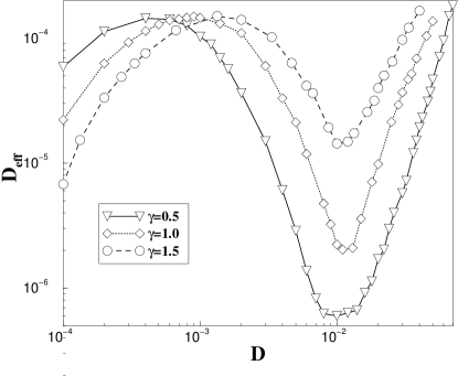
Figure 11: Effective phase diffusion coefficient vs. noise intensity for the periodically driven bistable Kramers oscillator Eq. (76) with angular driving frequency $\Omega=0.01$, driving amplitude $F=0.384$, which is close-to-threshold driving, and for different values of $\gamma$. For smaller values of the friction coefficient $\gamma$ phase diffusion is diminished.

The phase diffusion coefficient displays a local minimum that gets more pronounced if the damping coefficient $\gamma$ is decreased. Indeed, phase synchronization reveals itself through this local minimum of the average phase diffusion coefficient $D_{\rm eff}$ in the very region of the noise intensity $D$ where we also observe frequency synchronization, cf. Fig. 9.

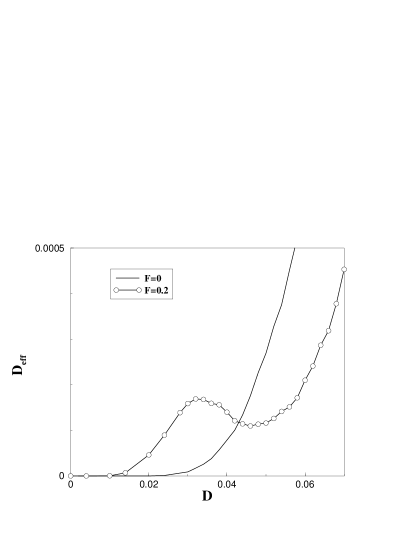
Figure 12: Effective phase diffusion coefficient vs. noise intensity for the periodically driven bistable Kramers oscillator Eq. (76) with friction coefficient $\gamma=0.5$, angular driving frequency $\Omega=0.01$, plotted for the undriven case $F=0$ and for driving with an amplitude $F=0.2$.

The qualitative behaviour of the diffusion coefficient agrees also with a recently found result related to diffusion of Brownian particles in biased periodic potentials fnl . A necessary condition for the occurrence of a minimum was an anharmonic potential in which the motion takes place. In this biased anharmonic potential the motion over one period consists of a sequence of two events. Every escape over a barrier (Arrhenius-like activation) is followed by a time scale induced by the bias and describing the relaxation to the next minimum. The second step is weakly dependent on the noise intensity and the relaxation time may be even larger then the escape time as a result of the anharmonicity. For such potentials the diffusion coefficient exhibits a minimum for optimal noise, similar to the one presented in Figs. 11 and 12.

The average duration of locking episodes $\langle T_{\rm lock}\rangle$ can be computed by equating the second moment of the phase difference (between the driving signal and the oscillator) to $\pi^{2}$ FreuNeiLsg2001 . A rough estimate, valid for the regions where frequency synchronization occurs, i.e., where the dynamics of the phase difference is dominated by diffusion, thus reads $\langle T_{\rm lock}\rangle=\pi^{2}/D_{\rm eff}$ or, when expressed by the number of driving periods pfish

$$\langle n_{\rm lock}\rangle={\Omega\;\pi\over 2\;D_{\rm eff}}\,.$$ (86)

In this way we estimate from Figs. 11 and 12 $\langle n_{\rm lock}\rangle\sim 150\ldots 15000$ for $\Omega=0.01$ and relevant $D_{\rm eff}$ varying between $10^{-4}\ldots 10^{-6}$.

V.3 SR without noise-enhanced phase coherence

In the previous examples we have shown how frequency synchronization, revealing itself through a plateau of the output frequency matching the harmonic input frequency, and reduced phase diffusivity together mark the occurrence of noise-enhanced phase coherence. Optimal noise intensities were found in the range where one also observes SR (in the overdamped system). In order to underline that under certain conditions SR exists but may not be accompanied by effective phase synchronization we present simulation results for the Rice frequency and the diffusion coefficient in Fig. 13 obtained for the bistable Kramers oscillator with a friction coefficient $\gamma=1$ and external frequency $\Omega=0.1$.

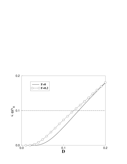
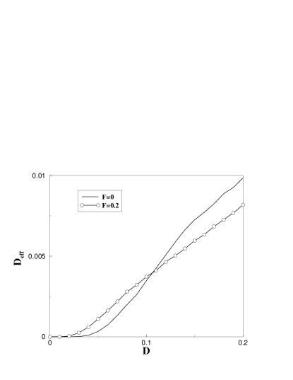
Figure 13: For friction coefficient $\gamma=1$ and external driving frequency $\Omega=0.1$ the bistable Kramers oscillator does neither exhibit frequency synchronization nor noise-enhanced phase coherence but still stochastic resonance occurs for noise intensities in the range of values ($D\approx 0.15$) where $\langle\omega\rangle_{R}\approx\Omega$.

For noise intensities $D\approx 0.15$ the output frequency matches $\Omega$ and nearby the overdamped Kramers oscillator exhibits the phenomenon of SR, i.e., one finds a maximum of the spectral power amplification SR_rev1 ; SR_rev2 . In contrast, we neither can find a minimum in the diffusion coefficient nor a plateau around $\Omega$ meaning that no phase coherence and not even frequency synchronization can be observed. The reason is that the external signal switches much too fast for the bistable system to follow; note that in the two-state description with Arrhenius rates the prefactor $\alpha_{0}$ (cf. Eq. 19) restricts the switching frequency from above. Noise-induced phase coherence requires a device with a faster internal dynamics, i.e., $\Omega\ll\alpha_{0}$.

VI Conclusions

We underline that the noise-induced phase synchronization is a much more stringent effect than stochastic resonance. This statement becomes most obvious when recalling that the spectral power amplification attains a maximum at an optimal noise intensity for arbitrarily small signal amplitudes and any frequency of the external signal. In contrast, noise-induced phase synchronization and even frequency locking are nonlinear effects and as such require amplitude and frequency to obey certain bounds (see the “Arnold tongues” in Sec. III). We expect that the functioning of important natural devices, e.g. communication and information processing in neural systems or sub-threshold signal detection in biological receptors, rely on phase synchronization rather than stochastic resonance.

- [1] V. I. Arnold, Trans. of the Am. Math. Soc. 42, 213 (1965); E. Ott, Chaos in Dynamical Systems, (Cambridge University Press, Cambridge, 1993).
- [2] R.L. Stratonovich, Topics in the Theory of Random Noise, (Gordon and Breach, New York, 1967).
- [3] H. Fujisaka and T. Yamada, Prog. Theor. Phys.69, 32 (1983); A.S. Pikovsky, Z. Phys. B 55, 149 (1984); L.M. Pecora and T.L. Carroll, Phys. Rev. Lett. 64, 821 (1990).
- [4] N.F. Rulkov, M.M. Sushchik, L.S. Tsimring, and H.D.I. Abarbanel, Phys. Rev. E 51, 980 (1995); L. Kocarev and U. Parlitz, Phys. Rev. Lett 76, 1816 (1996).
- [5] M.G. Rosenblum, A.S. Pikovsky, and J. Kurths, Phys. Rev. Lett. 78, 4193 (1997); S. Taherion and Y.C. Lai, Phys. Rev. E 59, R6247 (1999);
- [6] M.G. Rosenblum, A.S. Pikovsky, and J. Kurths, Phys. Rev. Lett. 76, 1804 (1996).
- [7] S.K. Han, T.G. Yim, D.E. Postnov, and O.V. Sosnovtseva, Phys. Rev. Lett. 83, 1771 (1999).
- [8] E.M. Izhikevich, Int. J. Bifur. Chaos 10, 1171 (2000); Bambi Hu and Changsong Zhou, Phys. Rev. E 63, 026201 (2001).
- [9] V. Anishchenko, A. Neiman, A. Astakhov, T. Vadiavasova, and L. Schimansky-Geier, Chaotic and Stochastic Processes in Dynamic Systems, (Springer, Berlin, 2002).
- [10] L. Schimansky-Geier, V. Anishchenko, and A. Neiman, in Neuro-informatics, S. Gielen and F. Moss (eds.), Handbook of Biological Physics, Vol. 4, Series Editor A.J. Hoff, (Elsevier Science, 2001).
- [11] A. Neiman, X. Pei, D. Russell, W. Wojtenek, L. Wilkens, F. Moss, H.A. Braun, M.T. Huber, and K. Voigt, Phys. Rev. Lett. 82, 660 (1999), S. Coombes and P.C. Bressloff, Phys. Rev. E 60, 2086 (1999) and Phys. Rev. E 63, 059901 (2001); W. Singer, Neuron 24, 49 (1999); R.C. Elson, A.I. Selverston, R. Huerta, N.F. Rulkov, M.I. Rabinovich, and H.D.I. Abarbanel, Phys. Rev. Lett. 81, 5692 (1998); P. Tass, M.G. Rosenblum, J. Weule, J. Kurths, A. Pikovsky, J. Volkmann, A. Schnitzler, and H.-J. Freund, Phys. Rev. Lett. 81, 3291 (1998); R. Ritz and T.J. Sejnowski, Current Opinion in Neurobiology 7, 536 (1997).
- [12] B. Schäfer, M.G. Rosenblum, and J. Kurths, Nature (London) 392, 239 (1998).
- [13] B. Blasius, A. Huppert, and L. Stone, Nature (London) 399, 354 (1999).
- [14] J.P.M. Heald and J. Stark, Phys. Rev. Lett. 84, 2366 (2000).
- [15] J.A. Freund, A.B. Neiman, and L. Schimansky-Geier, Europhys. Lett. 50, 8 (2000).
- [16] L. Callenbach, P. Hänggi, S.J. Linz, J.A. Freund, L. Schimansky-Geier, Phys. Rev. E (in press).
- [17] S.O. Rice, Bell System Technical J., 23 /24, 1 - 162 (1944/1945); note Sec. 3.3 on p. 57 - 63 in this double volume therein.
- [18] S.O. Rice, in Selected Papers on Noise and Stochastic Processes, N. Wax, ed., pp. 189-195 therein, (Dover, New York, 1954)
- [19] L. Gammaitoni, P. Hänggi, P. Jung, and F. Marchesoni, Rev. Mod. Phys. 70, 223 (1998).
- [20] V.S. Anishchenko, A.B. Neiman, F. Moss, and L. Schimansky-Geier, Phys. Usp. 42, 7 (1999).
- [21] A. Neiman, A. Silchenko, V. Anishchenko, and L. Schimansky-Geier, Phys. Rev. E 58, 7118 (1998).
- [22] P. Jung, Phys. Rep. 234, 175 (1995).
- [23] N.N. Bogoliubov and Y.A. Mitropolski, Asymptotic Methods in the Theory of Non-Linear Oscillations, (Gordon and Breach Sciences Publishers, New York, 1961).
- [24] The explicit expression for the phase involving the has to be understood in the sense of adding multiples of to make it a continuously growing function of time.
- [25] P. Hänggi and P. Riseborough, Am. J. Phys. 51, 347 (1983).
- [26] The statement requires the function defined in Eq. (2) to remain finite for ; this, however, is no severe restriction.
- [27] A.T. Winfree, J. Theor. Biol., 16 15 (1967); J. Guckenheimer, J. Math. Biol. 1, 259 (1975).
- [28] D. Gabor, J. IEE (London) 93 (III), 429 (1946).
- [29] A. Pikovsky, M. Rosenblum, and J. Kurths, Synchronization: A Universal Concept in Nonlinear Sciences, (Cambridge University Press, Cambridge, 2001).
- [30] L.A. Vainstein and D.E. Vakman, Frequency Analysis in the Theory of Oscillations and Waves (in Russian), (Nauka, Moscow, 1983).
- [31] R. Carmona, W.-L. Hwang, B. Torresani, Practical Time-Frequency Analysis, (Academic Press, San Diego, 1998).
- [32] J.-P. Lachaux, E. Rodriguez, M. Le Van Quen, A. Lutz, J. Martinerie, and F. Varela, Int. J. Bifur. Chaos 10, 2429 (2000); M. Le Van Quen, J. Foucher, J.-P. Lachaux, E. Rodriguez, A. Lutz, J. Martinerie, and F. Varela, J. Neurosci. Meth. 111, 83 (2001).
- [33] D.J. DeShazer, R. Breban, E. Ott, and R. Roy, Phys. Rev. Lett. 87, 044101 (2001).
- [34] B. McNamara and K. Wiesenfeld, Phys. Rev. A 39, 4854 (1989).
- [35] D.R. Cox, Renewal Theory, (Chapman & Hall, London, 1967).
- [36] J.A. Freund, A.B. Neiman, and L. Schimansky-Geier, in P. Imkeller and J. von Storch (eds.), Stochastic Climate Models. Progress in Probability, (Birkhäuser, Boston, Basel, 2001).
- [37] N. G. van Kampen, Stochastic Processes in Physics and Chemistry rev. and enl. ed. (North-Holland, Amsterdam, 1992).
- [38] R. Adler, Proc. IRE 34, 351 (1946); P. Hänggi and P. Riseborough, Am. J. Phys. 51, 347 (1983).
- [39] C. Van den Broeck, Phys. Rev. E 47, 4579 (1993); U. Zürcher and C. R. Doering, Phys. Rev. E 47, 3862 (1993).
- [40] F. Marchesoni, F. Apostolico, and S. Santucci, Phys. Rev. E 59, 3958 (1999).
- [41] A. Neiman, L. Schimansky-Geier, F. Moss, B. Shulgin, and J. J. Collins, Phys. Rev. E 60, 284 (1999).
- [42] B. Shulgin, A. Neiman, and V. Anishchenko, Phys. Rev. Lett. 75, 4157 (1995).
- [43] R. Rozenfeld, J.A. Freund, A. Neiman, L. Schimansky-Geier, Phys. Rev. E 64, 051107 (2001).
- [44] P. Hänggi, P. Talkner, and M. Borkovec, Rev. Mod. Phys. 62, 251 (1990).
- [45] P. Hänggi and H. Thomas, Phys. Rep. 88, 207 (1982); see sec. 2.4 therein.
- [46] P. Hänggi and P. Jung, Adv. Chem. Phys. 89, 239 (1995); P. Hänggi, F. Marchesoni, and P. Grigolini, Z. Physik B56, 333 (1984).
- [47] R. Benzi, G. Parisi, and A. Vulpiani, J. Phys. A: Math Gen. 14, L453 (1981); C. Nicolis, Solar Physics 74, 473 (1981).
- [48] A. Neiman, L. Schimansky-Geier, F. Moss, B. Shulgin, and J. J. Collins, Phys. Rev. E 60 , 284 (1999).
- [49] B. Lindner, M. Kostur and L. Schimansky-Geier, Fluct. and Noise Letters 1, R25 (2001).
- [50] J.A. Freund, J. Kienert, L. Schimansky-Geier, B. Beisner, A. Neiman, D.F. Russell, T. Yakusheva, and F. Moss, Phys. Rev. E 63, 031910 (2001).