Temperature-dependent quasiparticle band structure of the ferromagnetic semiconductor EuS

Abstract

We present calculations for the temperature-dependent electronic structure of the ferromagnetic semiconductor EuS. A combination of a many-body evaluation of a multiband Kondo-lattice model and a first-principles $T=0$–bandstructure calculation (tight-binding linear muffin-tin orbital (TB-LMTO)) is used to get realistic information about temperature- and correlation effects in the EuS energy spectrum. The combined method strictly avoids double-counting of any relevant interaction. Results for EuS are presented in terms of spectral densities, quasiparticle band structures and quasiparticle densities of states, and that over the entire temperature range.

I Introduction

Since the 1960s the europium chalcogenides EuX (X=O, S, Se, Te) have attracted tremendous research activity, experimentally as well as theoretically.Wachter79A ; Zinn76 ; Nol79a They are magnetic semiconductors, which crystallize in the rocksalt structure with increasing lattice constants (5 to 7Å) when going from the oxide to the telluride. The Eu²⁺ ions occupy lattice sites of an fcc structure so that each ion has twelve nearest and six next-nearest Eu-neighbors.

As to their purely magnetic properties the EuX are considered almost ideal realizations of the Heisenberg model for the so-called local-moment magnetism. Their magnetism is due to the half-filled 4f shell of the Eu²⁺. The 4f charge density distribution is nearly completely located within the filled $5s^{2}$ and $5p^{6}$ shells so that the overlap of 4f wavefunctions of adjacent Eu²⁺ ions is negligibly small. Hund s rules of atomic physics can be applied yielding an ${}^{8}S_{7/2}$ ground state configuration of the 4f shell. The $7\mu_{B}$ moments are exchange coupled resulting in antiferromagnetic (EuTe, EuSe), ferrimagnetic (EuSe), and ferromagnetic (EuO, EuS) orderings at low temperatures. The fact that the magnetic contribution to the thermodynamics of the EuX is excellently described by the Heisenberg Hamiltonian

$$H=-\sum_{i,j}J_{ij}\mathbf{S}_{i}\cdot\mathbf{S}_{j}$$ (1)

allows to test models of the microscopic coupling mechanism by direct comparison to experimental data. There is convincing evidence that the exchange integrals can be restricted to nearest ($J_{1}$) and next nearest neighbors ($J_{2}$)BZDK80 ; BKZ84 . $J_{1}$ is positive (ferromagnetic) decreasing from the oxide to the telluride. $J_{2}$ is negative, except for EuO, where the antiferromagnetic coupling increases in magnitude from the sulfide to the telluride. Liu and coworkersLiu80 ; Liu83 ; LL83 ; LL84 have proposed an indirect exchange between the localized 4f moments mediated by virtual excitations of chalcogenide-valence band (p) electrons into the empty Eu²⁺(5d) conduction bands together with a subsequent interband exchange interaction of the d electron (p hole) with the localized 4f electrons. Using this picture, very similar to the Bloembergen-Rowland mechanismbloembergen95 , the calculated values for $J_{1}$, $J_{2}$ agree nicely with experimental data, both in sign as well as in magnitude, for EuO, EuS, and EuSe. The results are found by a perturbative calculation of the indirect 4f-4f exchange interaction (1) with data from a linear combination of atomic orbitals (LCAO) method as band structure input. The different distances of the 4f moments do obviously create the different magnetic behavior of the EuX. For the exchange integrals of the two ferromagnets one finds:BZDK80 ; BKZ84

$$\mathrm{EuO:}\quad\frac{J_{1}}{k_{\mathrm{B}}}=0.625\mathrm{K};\quad\frac{J_{2}}{k_{\mathrm{B}}}=0.125\mathrm{K}$$ (2)

$$\mathrm{EuS:}\quad\frac{J_{1}}{k_{\mathrm{B}}}=0.221\mathrm{K};\quad\frac{J_{2}}{k_{\mathrm{B}}}=-0.100\mathrm{K}$$ (3)

Although in EuO the ferromagnetic interaction is more pronounced ($T_{\mathrm{C}}(\mathrm{EuO})=69.33$K; $T_{\mathrm{C}}(\mathrm{EuS})=16.57$K)Wachter79A a greater variety of experiments has been carried out with EuS than with EuO. The reason is that single crystals as well as films with well defined thicknessesgoncharenko98 ; stachow-wojcik99:_ferrom_eus_pbs can better be prepared for EuS than for EuO. Apart from this, the ferromagnetism of EuS is interesting in itself for two reasons. There are competing exchange integrals $J_{1}$ and $J_{2}$, and the magnitude of the dipolar energy is comparable to the exchange energy.

Besides the purely magnetic properties a striking temperature dependence of the (empty) conduction bands has caused intensive investigation. This was first detected for the ferromagnetic EuX as red-shift of the optical absorption edge (4f-5d) upon cooling below $T_{\mathrm{C}}$batlogg75 . The reason is an interband exchange coupling of the excited 5d electron to the localized 4f electrons that induces the temperature dependence of the localized moment system into the the empty conduction band states. A further striking effect, which is due to the induced temperature dependence of the conduction band states, is a metal-insulator transition observed in Eu-rich EuOpenny72 ; torrance72 . The Eu richness manifests itself in twofold positively charged oxygen vacancies. One of the two Eu²⁺ excess electrons, which are no longer needed for the binding, is thought to be tightly trapped by the vacancy. Because of the Coulomb repulsion, the other electron occupies an impurity level fairly close to the lower band edge. With decreasing temperature below $T_{c}$ the band edge crosses the impurity level thereby freeing impurity electrons. A conductivity jump as much as 14 orders of magnitude was observedtorrance72 . Other remarkable effects result from the interaction of the band electron with collective excitations of the moment system. One of these is the creation of a characteristic quasiparticle (magnetic polaron) which can be identified as a propagating electron dressed by a virtual cloud of excited magnons.

In previous papers we have proposed a method for the determination of the temperature dependent electronic structure of bulk EuOschiller01:_temper_euo as well as EuO-filmsschiller01:_kondo . The treatment is based on a combination of a multiband Kondo-lattice model (MB-KLM) with first principles tight-binding linear muffin-tin orbital (TB-LMTO) band structure calculations. The many-body treatment of the (ferromagnetic) KLM was combined with the first-principles part by strictly avoiding a double-counting of any relevant interaction. The most striking result concerned the prediction of a surface state for thin EuO(100) films, the temperature shift of which may cause a surface halfmetal-insulator transitionschiller01:_predic_euo . For low enough temperatures the shift of the surface state leads to an overlap with the occupied localized 4f states. Therefore, one can speculate that the resistivity of the EuO(100) films might be highly magnetic field dependent, so that a colossal magnetoresistance effect is to be expected.

In this paper we investigate in a similar manner the other ferromagnet EuS, where we restrict ourselves first to the bulk material. We want to derive the temperature dependent quasiparticle band structure (Q-BS), in particular concentrating on those effects, which are due to a mutual influence of localized magnetic 4f states and itinerant, weakly correlated conduction band states. There was earlier work on the Q-BS of bulk EuSborstel87 ; mathi00:_temper_eus . In these papers, however, an approach was employed that decomposes the Eu-5d band into five consecutive non-degenerate subbands. For each of the subbands a single-band KLM was evaluated therewith disregarding the full multiband-structure of the EuS conduction band. Obviously this procedure leads to an overestimation of certain correlation effects as a consequence of certainly too narrow subbands. We therefore use in this paper a multiband 4f-5d Kondo-lattice model to get reliably the temperature dependent Q-BS of EuS with all correlation effects in a symmetry-conserving manner. Our method combines a many-body analysis of the mentioned multiband-model with a self-consistent LMTO band structure calculation.

Since the technical details can be taken from schiller01:_temper_euo we present in the following only the general procedure together with those aspects which are vital for the understanding of the new EuS results. In Section 2 we formulate the multiband Hamiltonian and fix its single-particle part by a realistic band structure calculation. Furthermore, we describe the parameter choice for the decisive interband exchange coupling. Section 3.1 is devoted to the local-moment ferromagnetism of EuS, while Section 3.2 repeats shortly how we solved the multiband Kondo-lattice model. In Section 4 the electronic EuS structure is discussed in terms of quasiparticle band structures and densities of states (Q-DOS) as well as spectral densities, which are closely related to the angle and spin resolved (inverse) photoemission experiment.

II Multiband Kondo-Lattice Model

The complete model-Hamiltonian for a real substance with multiple conduction bands consists of three parts:

$$H=H_{5d}+H_{4f}+H_{df}$$ (4)

The first term contains the 5d conduction band structure of the considered material as, e.g., EuS:

$$H_{5d}=\sum_{i,j}\sum_{m,m^{\prime}}T_{ij}^{mm^{\prime}}c^{\dagger}_{im\sigma}c_{jm^{\prime}\sigma}$$ (5)

The indices m and m’ refer to the respective 5d subbands, i and j to lattice sites. c${}_{im\sigma}^{\dagger}$ and c_imσ are, respectively, the creation and annihilation operator for an electron with spin $\sigma$ ($\sigma=\uparrow,\downarrow$) from subband m at lattice site $\mathbf{R}_{i}$. $T_{ij}^{mm^{\prime}}$ are the hopping integrals, which are to be obtained from an LDA calculation in order to incorporate in a realistic manner the influences of all those interactions which are not directly accounted for by our model Hamiltonian.

Each site $\mathbf{R}_{i}$ is occupied by a localized magnetic moment, represented by a spin operator $\mathbf{S}_{i}$. It stems from the half-filled 4f shell of the Eu²⁺ ion, according to Hund’s rule being a pure spin moment of $7\mu_{B}$. The exchange coupled localized moments are described by an extended Heisenberg Hamiltonian

$$H_{4f}=-\sum_{ij}J_{ij}\mathbf{S}_{i}\cdot\mathbf{S}_{j}-D_{0}\sum_{i}\left(S_{i}^{z}\right)^{2}$$ (6)

In the case of EuS the exchange integrals $J_{ij}$ can be restricted to nearest and next nearest neighbors (3). The non-negligible dipolar energy in EuS is expressed by a single-ion anisotropy $D_{0}$.

The characterizing feature of the normal single-band KLM, also called s-f or s-d model, is an intraatomic exchange between conduction electrons and localized spins. The form of the respective multiband-Hamiltonian can be derived from the general on-site Coulomb interaction between electrons of different subbands. It was shown in schiller01:_temper_euo ; schiller01:_kondo that in the special case of EuX (half-filled 4f shell, empty conduction band) the interband exchange can be written as:

$$H_{df}=-\frac{1}{2}J\sum_{im}\Big{(}S_{i}^{z}\left(n_{im\uparrow}-n_{im\downarrow}\right)$$

$$+S_{i}^{+}c_{im\downarrow}^{\dagger}c_{im\uparrow}+S_{i}^{-}c_{im\uparrow}^{\dagger}c_{im\downarrow}\Big{)}$$

J is the corresponding coupling constant, and furthermore:

$$n_{im\sigma}=c^{\dagger}_{im\sigma}c_{im\sigma};\mbox{ }S^{\pm}=S^{x}\pm\mathrm{i}S^{y}$$ (8)

The first term in (II) represents an Ising type interaction while the two others refer to spin exchange processes. The latter are responsible for some of the most typical KLM properties.

In order to incorporate in a certain sense all those interactions, which are not directly covered by the model Hamiltonian, we take the hopping integrals from a band structure calculation according to the TB-LMTO-atomic sphere program of Andersenandersen75 ; andersen84 . In this method, the original Hamiltonian is transformed to a tight–binding Hamiltonian containing nearest neighbor correlations, only. The transformation is obtained by linearly combining the original muffin-tin orbitals to the short ranged tight–binding muffin-tin orbitals. The evaluation is restricted to 5d bands, only. LDA-typical difficulties arise with the strongly localized character of the 4f levels. To circumvent the problem we considered the 4f electrons as core electrons, since our main interest is focused on the reaction of the conduction bands on the magnetic state of the localized moments. For our purpose the 4f levels appear only as localized spins in the sense of $H_{4f}$ in Eq.(6). Figure 1 shows the calculated spin-dependent band structure of EuS, where, of course, the 4f levels are missing. Clearly,

Figure 1: Spin dependent (solid lines up-spin, broken lines down-spin) bandstructure of bulk EuS calculated within a TB-LMTO scheme with the 4f levels treated as core states. The energy zero coincides with the Fermi energy.

the conduction-band region is dominated by Eu-5d states. For our subsequent model calculations it is therefore reasonable to restrict the single-particle input from the band structure calculations to the Eu-5d part, only. The low-energy part in Figure 1 belongs to the S-3p states. For comparison we have also performed an LDA+U calculation which is able to reproduce the right positions of the respective bands. However this method suffers from the introduction of adjustable parameters $U$ and $J$ being, therefore, no longer a “first principles” theory. The results of the LDA+U calculation do not differ strongly from those of the “normal” LDA, with the 4f electrons treated as core electrons. So we have chosen the much simpler LDA calculation. Since we are mainly interested in overall correlation and temperature effects, the extreme details of the bandstructure are surely not so important. In Figure 2, from the same calculation, the LDA-density of states is displayed. A distinct exchange splitting is visible which can be used to fix the interband exchange coupling constant J in Eq.(II). Assuming that

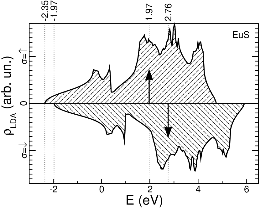
Figure 2: Spin-dependent density of 5d-states of EuS as function of energy (calculated within a TB-LMTO scheme). The numbers are (in eV) for the lower band edges and for the centers of gravity. The Fermi edge is below the 5d band (see Fig. 1).

an LDA treatment of ferromagnetism is quite compatible with the Stoner (mean field) picture, as stated by several authorsjanack76 ; poulsen76 , the $T=0$ splitting should amount to $\Delta E=JS$. Unfortunately, the results in Figure 2 do not fully confirm this simple assumption but rather point to an energy-dependent exchange splitting. The indicated shifts of the lower edge and of the center of gravity lead to different $J$ values:

$$J=J(\mathrm{edge})=0.11\mathrm{eV};\quad J=J(\mathrm{center})=0.23\mathrm{eV}$$ (9)

In the following we will use both values for the a bit oversimplified ansatz $H_{df}$ in Eq.(II) to compare the slightly different consequences.

It is a well-known fact (see Figure 1 in meyer01:_quant_kondo and further references there) that the KLM can exactly be solved for the ferromagnetically saturated ($T=0$) semiconductor. It is found that the $\uparrow$ spectrum is rigidly shifted towards lower energies by the amount of $\frac{1}{2}JS$, while the $\downarrow$ spectrum is remarkably deformed by correlation effects due to spin exchange processes between extended 5d and localized 4f states. We cannot switch off the interband exchange interaction $H_{df}$ in the LDA code, but we can exploit from the exact $T=0$ result that it leads in the $\uparrow$ spectrum only to an unimportant rigid shift. So we take from the LDA calculation, which holds by definition for $T=0$, the $\uparrow$ part as the single-particle input for $H_{5d}$ in Eq.(5). Therewith it is guaranteed that all the other interactions, which do not explicitly enter the KLM operator (4), are implicitly taken into account by the LDA-renormalized single-particle Hamiltonian (5). On the other hand, a double counting of any decisive interaction is definitely avoided.

III Model Evaluation

III.1 Magnetic Part

Because of the empty conduction bands the magnetic ordering of the localized 4f moments will not directly be influenced by the band states. For the purely magnetic properties of EuS it is therefore sufficient to study exclusively the extended Heisenberg-Hamiltonian (6). While the exchange integrals $J_{ij}$ are known from spin wave analysis (see Eq.(3)), the single-ion anisotropy constant $D_{0}$ must be considered an adjustable parameter. Via the magnon-Green function

$$P_{ij}(E)=\langle\langle S_{i}^{+};S_{j}^{-}\rangle\rangle$$ (10)

we can calculate all desired f spin correlation functions by evaluating the respective equation of motion:

$$EP_{ij}(E)=2\hbar^{2}\left<S_{i}^{z}\right>\delta_{ij}+\left\langle\left\langle\left[S_{i}^{+},H_{4f}\right]_{-};S_{j}^{-}\right\rangle\right\rangle_{E}$$ (11)

Evaluation of this equation of motion requires the decoupling of higher Green functions, originating from the Heisenberg exchange term and the anisotropy part in Eq.(6). For Green functions coming out of the Heisenberg term we have used the so-called Tyablikow approximation, which is known to yield reasonable results in all temperature regions. For Green functions, which arise from the anisotropy term, we use a decoupling technique proposed by LinesLin67 . Details of the method have been presented in a previous paperschiller99:_thick_curie_heisen on EuO. As result one gets the following well-known expression for the temperature dependent local-moment magnetization:

$$\left<S^{z}\right>=\hbar\frac{(1+\phi)^{2S+1}(S-\phi)+\phi^{2S+1}(S+1+\phi)}{\phi^{2S+1}-(1+\phi)^{2S+1}}$$ (12)

$\phi$ can be interpreted as average magnon number:

$$\phi=\frac{1}{N}\sum_{\mathbf{k}}\left(e^{\beta E(\mathbf{k})}-1\right)^{-1},$$ (13)

where $E(\mathbf{k})$ is the pole of the wave vector dependent Fourier transform of $P_{ij}(E)$. Some typical magnetization curves are plotted in Figure 3. They differ by the value of the anisotropy constant $D_{0}$, which is still an undetermined parameter. When $D_{0}/k_{\mathrm{B}}$ increases from $0.01$K to $0.4$K $T_{\mathrm{C}}$ rises from about $15$K to $16.9$K. Regarding that $J_{1}$, $J_{2}$ are derived from a low-temperature spin-wave fit, the agreement between the calculated $T_{c}$s and the experimental value of $16.57\mathrm{K}$Wachter79A is remarkably good for almost all applied values of $D_{0}$, and best for $0.375\mathrm{K}$. Since we

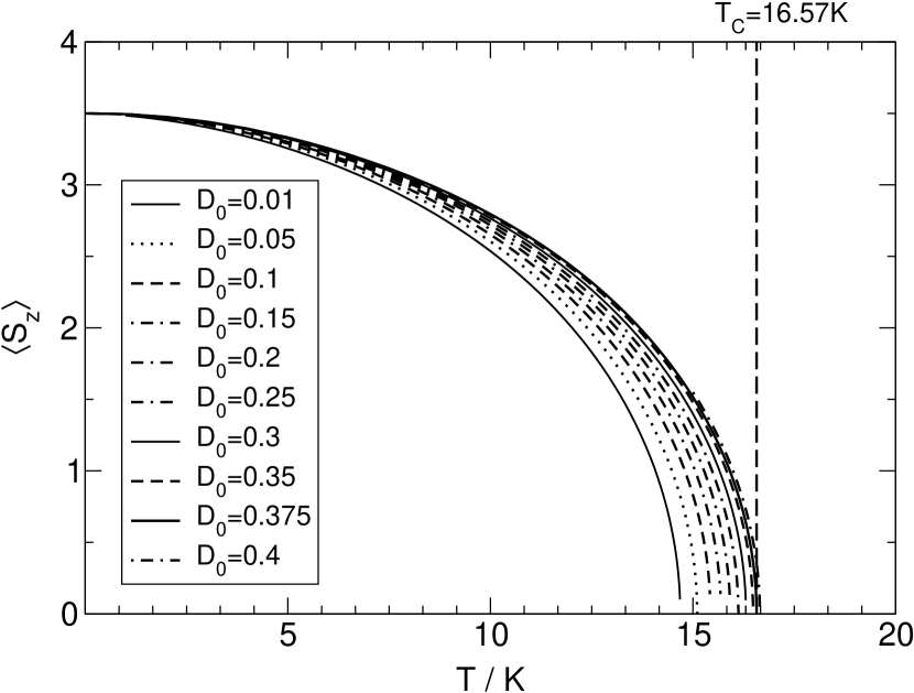
Figure 3: 4f-magnetization as a function of temperature for various values of the single–ion anisotropy $D_{0}$. The vertical broken line marks the used experimental value ($T_{\mathrm{C}}=16.57\mathrm{eV}$).

are interested above all in the electronic bulk band structure and its temperature dependence, the actual numerical value of $D_{0}$ does not play the decisive role. However, when treating systems of lower dimensionality (films, surfaces), which is planned for a forthcoming paper, then a finite $D_{0}$ will be the precondition for getting a collective magnetic order of the spin systemMW66 ; gelfert01 .

Together with (12) and (13) practically all local spin correlations are derivable, as e.g.:

$$\left<S^{-}S^{+}\right>=2\hbar\left<S^{z}\right>\phi$$ (14)

$$\left<(S^{z})^{2}\right>=\hbar^{2}S(S+1)\left<S^{z}\right>(1+2\phi)$$ (15)

$$\left<(S^{z})^{3}\right> = \hbar^{3}S(S+1)\phi+\hbar^{2}\left<S^{z}\right>(S(S+1)+\phi)$$ (16)

$$-\hbar\left<(S^{z})^{2}\right>(1+2\phi)$$

These and similar terms are responsible for the temperature dependence of the electronic selfenergy.

III.2 Electronic Part

The inspection of the electronic part starts from the retarded Green function $\langle\langle c_{im\sigma};c_{jm^{\prime}\sigma}^{\dagger}\rangle\rangle_{E}$ or its wave-vector dependent Fourier transform:

$$\hat{G}_{\mathbf{k}\sigma}(E)=\frac{\hbar}{E\mathbf{1}-\hat{T}_{\mathbf{k}}-\hat{\Sigma}_{\mathbf{k}\sigma}(E)}$$ (17)

Here $\mathbf{1}$ represents the $(M\times M)$ identity matrix, where M is the number of relevant subbands. The elements $T_{\mathbf{k}}^{mm^{\prime}}$ of the hopping matrix are the Fourier transforms of the hopping integrals in Eq.(5), while the elements of the selfenergy matrix are introduced by

$$\left\langle\left\langle\left[c_{im\sigma},H_{df}\right]_{-};c_{jm^{\prime}\sigma}^{\dagger}\right\rangle\right\rangle_{E}\equiv\sum_{lm^{\prime\prime}}\Sigma_{il\sigma}^{mm^{\prime\prime}}(E)G_{lj\sigma}^{m^{\prime\prime}m^{\prime}}(E)$$ (18)

with subsequent Fourier transformation.

To get explicitly the selfenergy elements in Eq.(18) we evaluate the commutator on the left-hand side what produces two higher Green functions:

$$\Gamma_{ikj\sigma}^{mm^{\prime}}(E)=\left\langle\left\langle S_{i}^{z}c_{km\sigma};c_{jm^{\prime}\sigma}^{\dagger}\right\rangle\right\rangle_{E}$$ (19)

$$F_{ikj\sigma}^{mm^{\prime}}(E)=\left\langle\left\langle S_{i}^{-\sigma}c_{km-\sigma};c_{jm^{\prime}\sigma}^{\dagger}\right\rangle\right\rangle_{E}$$ (20)

$\Gamma$ arises from the Ising type interaction in the d-f interaction term (II) and F from the spin exchange partial operator $(S^{\uparrow,\downarrow}=S^{+,-})$:

$$\left\langle\left\langle\left[c_{im\sigma},H_{df}\right]_{-};c_{jm^{\prime}\sigma}^{\dagger}\right\rangle\right\rangle_{E}=-\frac{1}{2}J\left(z_{\sigma}\Gamma_{iij\sigma}^{mm^{\prime}}+F_{iij\sigma}^{mm^{\prime}}\right)$$ (21)

$(z_{\sigma}=\delta_{\sigma\uparrow}-\delta_{\sigma\downarrow})$. Exploiting already the fact that the EuS conduction band is empty we encounter the following equations of motion of the higher Green functions (19) and (20):

$$\sum_{lm^{\prime\prime}}\left(E\delta_{kl}\delta_{mm^{\prime\prime}}-T_{kl}^{mm^{\prime\prime}}\right)\Gamma_{ilj\sigma}^{m^{\prime\prime}m^{\prime}}(E)=$$

$$\hbar\langle S^{z}\rangle\delta_{kj}\delta_{mm^{\prime}}+\left\langle\left\langle S_{i}^{z}\left[c_{km\sigma},H_{df}\right]_{-};c_{jm^{\prime}\sigma}^{\dagger}\right\rangle\right\rangle_{E}$$

$$\sum_{lm^{\prime\prime}}\left(E\delta_{kl}\delta_{mm^{\prime\prime}}-T_{kl}^{mm^{\prime\prime}}\right)F_{ilj\sigma}^{m^{\prime\prime}m^{\prime}}(E)=$$

$$\left\langle\left\langle(\delta_{\sigma\uparrow}S_{i}^{-}+\delta_{\sigma\downarrow}S_{i}^{+})\left[c_{km-\sigma},H_{df}\right]_{-};c_{jm^{\prime}\sigma}^{\dagger}\right\rangle\right\rangle_{E}$$

On the right-hand side of these equations appear further higher Green functions which prevent a direct solution and require an approximative treatment. That shall be different for the non-diagonal terms ($i\neq k$) and the diagonal terms ($i=k$), because the strong intraatomic correlations due to the on-site interaction (II) have to be handled with special care. For $i\neq k$ a self-consistent selfenergy approach is applied, which has been tested in numerous previous papersNRMJ97 ; NMJR96 ; schiller01:_temper_euo ; schiller01:_kondo ; meyer01:_quant_kondo ; schiller99:_thick_curie_heisen . It simply consists in treating the commutators in (III.2) and (III.2), respectively, in formal analogy to the definition equation (18) for the selfenergy:

$$\left\langle\left\langle S_{i}^{z}\left[c_{km\sigma},H_{df}\right]_{-};c_{jm^{\prime}\sigma}^{\dagger}\right\rangle\right\rangle_{E}\rightarrow\sum_{lm^{\prime\prime}}\Sigma_{il\sigma}^{mm^{\prime\prime}}\Gamma_{ilj\sigma}^{m^{\prime\prime}m^{\prime}}(E)$$ (24)

$$\left\langle\left\langle(\delta_{\sigma\uparrow}S_{i}^{-}+\delta_{\sigma\downarrow}S_{i}^{+})\left[c_{km-\sigma},H_{df}\right]_{-};c_{jm^{\prime}\sigma}^{\dagger}\right\rangle\right\rangle_{E}$$

$$\rightarrow\sum_{lm^{\prime\prime}}\Sigma_{il-\sigma}^{mm^{\prime\prime}}F_{ilj\sigma}^{m^{\prime\prime}m^{\prime}}(E)$$

For the diagonal terms ($i=k$) a moment technique is used that takes the local correlations better into account. For this purpose we explicitly evaluate the commutators in Eqs.(III.2),(III.2) obtaining then, as usual, further higher Green functions. In the first step these new functions are reduced to a minimum number by exploiting that all functions, arising from the Ising-equation (III.2), can rigorously be expressed by linear combinations of those which come out of the spinflip-equation (III.2). For a decoupling, the latter are then written as linear combinations of simpler functions that are already involved in the hierarchy of Green functions. The choice, which kind of simpler functions enter the respective ansatz, is guided by exactly solvable limiting cases (ferromagnetic saturation, zero-bandwidth limit, $S=\frac{1}{2}$). We illustrate the procedure by a typical example:

$$D_{ij\sigma}^{mm^{\prime}}(E)=\langle\langle\Delta_{i\sigma}c_{im\sigma};c_{jm^{\prime}\sigma}^{+}\rangle\rangle$$

$$\Delta_{i\sigma}=\delta_{\sigma\uparrow}S_{i}^{-}S_{i}^{+}+\delta_{\sigma\downarrow}S_{i}^{+}S_{i}^{-}$$ (26)

For $S=\frac{1}{2}$ it holds rigorously:

$$D_{ij\sigma}^{mm^{\prime}}(E)=\frac{1}{2}G_{ij\sigma}^{mm^{\prime}}(E)-(\delta_{\sigma\uparrow}-\delta_{\sigma\downarrow})\Gamma_{iij\sigma}^{mm^{\prime}}(E)$$ (27)

This relation is valid for all temperatures. On the other hand, in ferromagnetic saturation ($\langle S^{z}\rangle=S$) the same function reads for all spin values:

$$D_{ij\sigma}^{mm^{\prime}}(E)=SG_{ij\sigma}^{mm^{\prime}}(E)-(\delta_{\sigma\uparrow}-\delta_{\sigma\downarrow})\Gamma_{iij\sigma}^{mm^{\prime}}(E)$$ (28)

Eqs. (27) and (28) clearly suggest the following ansatz for the general case:

$$D_{ij\sigma}^{mm^{\prime}}(E)=\alpha_{\sigma}^{mm^{\prime}}G_{ij\sigma}^{mm^{\prime}}(E)+\beta_{\sigma}^{mm^{\prime}}\Gamma_{iij\sigma}^{mm^{\prime}}(E)$$ (29)

In order to fix the coefficients $\alpha_{\sigma}^{mm^{\prime}}$ and $\beta_{\sigma}^{mm^{\prime}}$, we now calculate the first two spectral moments of each of the three Green functions in (29), and that exactly and independently from the respective Green function. The diagonal parts of all other functions, appearing on the right-hand sides of (III.2) and (III.2), can be elaborated analogously.

By these manipulations we arrive at a closed system of equations for the selfenergy matrix elements $\Sigma_{ij\sigma}^{mm^{\prime}}(E)$, which can numerically be solved. Via the spectral moments, used for the various ansatze such as (29), a set of local spin correlations as those in Eqs.(12,14,15,16) enter the procedure. They are mainly responsible for the temperature-dependence of the electronic selfenergy.

To get a first impression of correlation effects in the electronic structure of EuS we have evaluated our complex theory for T=0K. The Q-DOS results are exhibited in Figure 4. As explained and tentatively justified before Eq.(9) we use two different values for the exchange

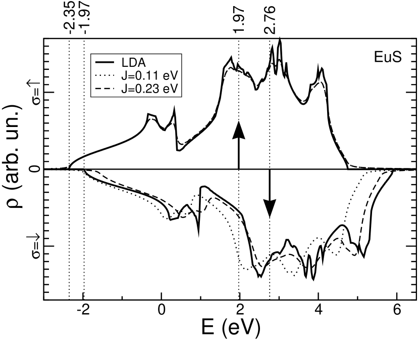
Figure 4: The same as in Fig. 2, but in addition the $T=0$ results of our combined many-body / first principles theory. The latter has been performed for two different values of the exchange coupling J (dotted line $J=0.11$eV; broken line $J=0.23$eV). The up-spin curves have been shifted both to coincide at the lower edge with the LSDA curve. That demonstrates that at $T=0$ correlation effects appear in the down–spectrum only.

coupling J. The $\uparrow$ Q-DOS is unaffected by the actual value of J and coincides with the respective LDA curve, when we compensate, as done in Figure 4, the unimportant rigid shift $(-\frac{1}{2}JS)$. So our approach fulfills the exact $(T=0,\sigma=\uparrow)$-limit. The slight deviations, seen in the upper part of Figure 4, are exclusively due to the numerical rounding procedure. A posteriori this fact demonstrates once more that our above-described method for implementing the LDA input into the many-body model calculation definitely circumvents the often discussed double counting problem. As explained in Section 2 we succeeded in this respect because for the special case of a ferromagnetically saturated semiconductor the $\uparrow$ spectrum is free of correlation effects which stem from the interband exchange $H_{df}$.

The lower half of Figure 4 demonstrates that correlation effects do appear, even at $T=0$K, in the $\downarrow$ spectrum. Besides a band narrowing, they provoke strong deformations and shifts with respect to the LDA result. Here the influence of the different J values from Eq.(9) is quite remarkable. For getting quantitative details of the EuS-energy spectrum a proper choice of the exchange constant is obviously necessary. The lower value $(J=0.11\mathrm{eV})$ is appropriate when we are mainly interested in the lower band-edge region. However, in the middle of the band, around the center of gravity, $J=0.23\mathrm{eV}$ is surely the better choice.

IV EuS Energy Spectrum

The main focus of our study is the temperature dependence of the 5d-energy spectrum of the ferromagnetic semiconductor EuS. The 5d bands are empty, except for the single test electron, so that the T-dependence must be exclusively caused by the exchange coupling of the band states to the localized magnetic 4f states. Figure 5 and Figure 6 display the quasiparticle densities of states for five different 4f magnetizations, i.e. five different temperatures (Figure 3). The Q-DOS in Figure 5 are calculated for $J=0.11\mathrm{eV}$. One sees that the lower

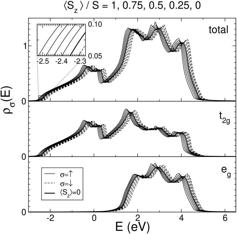
Figure 5: Quasiparticle densities of states of the Eu–5d bands of bulk EuS as a function of energy for various temperatures. Solid lines for up–spin, broken lines for down–spin, thick line for $T=T_{\mathrm{C}}$ ($\langle S^{z}\rangle$=0). The outermost curves belong to $T=0$ ($\langle S^{z}\rangle/S=1$). They approach each other when increasing the temperature. The inset shows on an enlarged scale the temperature shift of the lower up–spin edge. Exchange coupling: $J=0.11$eV.

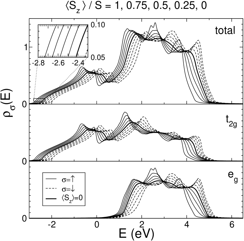
Figure 6: The same as in Fig. 5 but for $J=0.23$eV.

edge of the $\uparrow$ Q-DOS performs a shift to lower energies upon cooling from $T=T_{\mathrm{C}}$ down to $T=0\mathrm{K}$. This explains the famous red shift of the optical absorption edge for an electronic $4f-5d_{t_{2g}}$ transition, first observed by Busch and WachterWac64 ; BJW65 . We find a shift of about $0.17\mathrm{eV}$ (see inset in Figure 5),very close to the experimental dataWachter79A ; batlogg75 . This confirms once more that $J=0.11\mathrm{eV}$ is a realistic choice for the exchange coupling constant as long as the lower part of the 5d spectrum is under consideration. Note, that our fitting procedure for the exchange constant $J$ (Fig. 2, Eq. (9)) does not predetermine the redshift.

Since we have taken into account for our calculation the full band structure of the Eu-5d conduction bands, the symmetry of the different Eu-5d orbitals is preserved. The 5d bands of bulk EuS are therefore split into $t_{2g}$ and $e_{g}$ subbands (Figure 5), where the $t_{2g}$ bands are substantially broader ($\sim 7\mathrm{eV}$) than the $e_{g}$ bands ($\sim 4\mathrm{eV}$). In a previous study of the temperature dependent EuS-band structureborstel87 the Eu-5d complex was split into five s-like bands by numbering for a given $\mathbf{k}$ vector the states from m=1 to m=5 according to increasing single-electron energies $\epsilon_{m}(\mathbf{k})$. All $\mathbf{k}$ states with an energy $\epsilon_{m}(\mathbf{k})$ then form the subband m. This simplified procedure does not respect symmetries and neglects subband hybridization, i.e. interband hopping $T_{ij}^{mm^{\prime}}$ for $m\neq m^{\prime}$. The subband widths W turn out to be of order $1-3eV$ being therefore distinctly narrower than those in Figure 5. That has an important consequence. Since correlation effects scale with the effective(!) exchange coupling $\frac{J}{W}$, they become for the same J more pronounced in narrower bands. That is why we believe that correlations are to a certain degree overestimated in borstel87 . As a consequence of the weaker effective coupling the appearance of polaron-like quasiparticle branches is less likely in the present investigation.

In Figure 6 the Q-DOS is plotted for the stronger exchange coupling $J=0.23\mathrm{eV}$, which should be more realistic for the middle part of the spectrum, around the center of gravity. The temperature-influence on the spectrum is more pronounced than for the weaker coupling in Figure 5. Strong deformations and shifts appear, being not at all rigid, i.e. far beyond the mean field picture. However, not surprising, the lower edge shift between $T=T_{\mathrm{C}}$ and $T=0\mathrm{K}$ comes out too strong. The calculated red shift of $0.27\mathrm{eV}$ substantially exceeds the experimental value of $0.167\mathrm{eV}$Wachter79A . As mentioned above, the lower part of the spectrum is better described with $J=0.11\mathrm{eV}$.

While the Q-DOS refers to the spin resolved, but angle averaged (inverse) photoemission experiment, the $\mathbf{k}$ dependent spectral density is the angle resolved counterpart. From $S_{\mathbf{k}\sigma}(E)$ we derive the quasiparticle band structure (Q-BS).

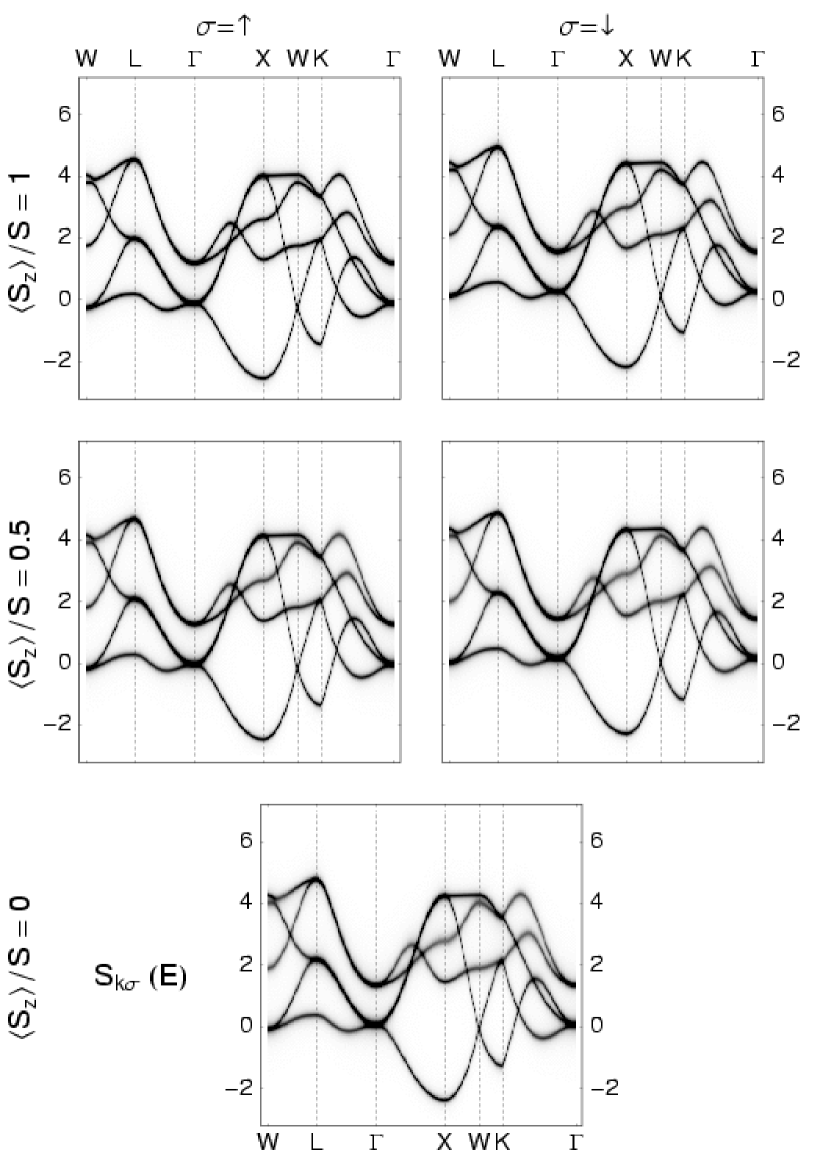
Figure 7: Spin–dependent quasiparticle bandstructure of the Eu–5d bands of bulk EuS for different 4f magnetizations $\langle S^{z}\rangle/S$. Exchange coupling: $J=0.11$eV.

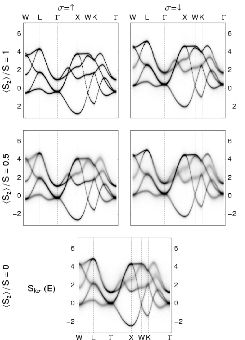
Figure 8: The same as in Fig. 7, but for $J=0.23$eV.

Figures 7 and 8 represent as density plots the spectral density for some symmetry directions. The degree of blackening is a measure of the magnitude of the spectral function. Figure 7 holds for $J=0.11\mathrm{eV}$ and Figure 8 for $J=0.23\mathrm{eV}$. In both situations the $\uparrow$ spectrum in case of ferromagnetic saturation coincides with the dispersions obtained from the LDA calculation. In the weak coupling case (Figure 7) the temperature influence is mainly a shift of the total spectrum. The induced exchange splitting reduces with increasing T and disappears at $T=T_{\mathrm{C}}$. Correlation effects are more clearly visible in the case of $J=0.23\mathrm{eV}$ (Figure 8). They manifest themselves above all in lifetime effects. Great parts of the dispersions are washed out because of magnon absorption (emission) of the itinerant $\uparrow(\downarrow)$ electron with simultaneous spinflip. In ferromagnetic saturation a $\uparrow$ electron has no chance to absorb a magnon because there does not exist any magnon. Therefore the dispersion appears sharp representing quasiparticles with infinite lifetime. On the other hand, the $\downarrow$ electron has even at $T=0\mathrm{K}$ the possibility to emit a magnon becoming then a $\uparrow$ electron. Therefore correlation effects are already at $T=0\mathrm{K}$ present in the $\downarrow$ spectrum. For finite temperatures, finite demagnetizations, magnons are available and absorption processes provoke quasiparticle damping in the $\uparrow$ spectrum, too. The overall exchange splitting reduces with increasing temperatures, until in the limit $T\rightarrow T_{c}$ ($\langle S^{z}\rangle\rightarrow 0$) the vanishing 4f magnetization removes the induced spin asymmetry in the 5d subbands.

Figure 9: Spin–dependent spectral density $S_{\mathbf{k}\sigma}$ of the Eu–5d states of bulk EuS as function of energy for the same 4f magnetizations as in Fig. 8. Solid lines: up–spin; broken lines: down–spin; thick lines: $T=T_{\mathrm{C}}$ ($\langle S^{z}\rangle=0)$). Exchange coupling: $J=0.23$eV; $\mathbf{k}=\Gamma$.

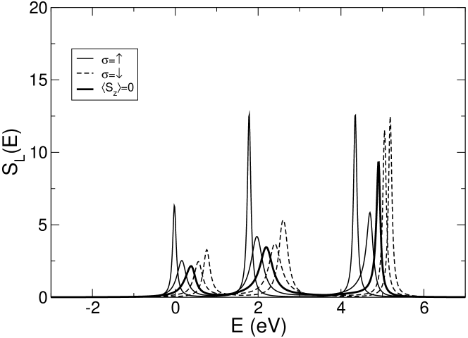
Figure 10: The same as in Fig. 9 but $\mathbf{k}=\mathrm{L}$.

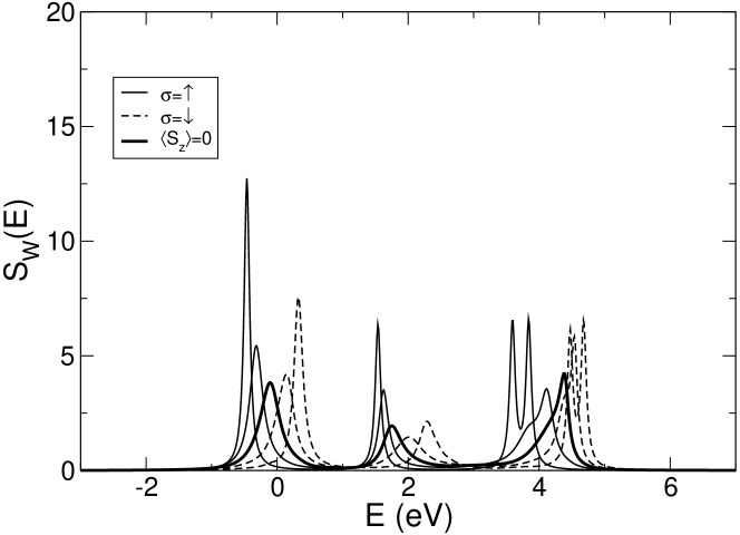
Figure 11: The same as in Fig. 9 but $\mathbf{k}=\mathrm{W}$.

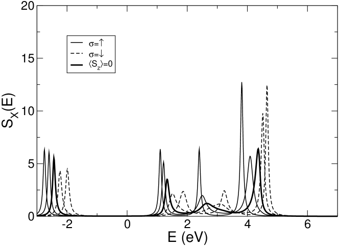
Figure 12: The same as in Fig. 9 but $\mathbf{k}=\mathrm{X}$.

For a better insight into the temperature-behavior we have plotted in Figs. 9–12 for four $\mathbf{k}$–points from the Brillouin zone ($\Gamma$, L, W, X) the energy dependence of the spectral density, and that for the same three temperatures as in Fig. 8. For the $\Gamma$–point we expect two structures according to the twofold (e_g) and threefold (t_2g) degenerate dispersions. As can be seen in Fig. 9 well defined quasi particle peaks appear with additional spin split below $T_{\mathrm{C}}$. The exchange splitting, introduced via the interband coupling to the magnetically active 4f system, collapses for $T\rightarrow T_{\mathrm{C}}$ (Stoner–like behavior). Obviously, quasiparticle damping increases with increasing temperature. Similar statements hold for the spectral density at the L–point. In accordance with the quasiparticle bandstructure in Fig. 8 three structures appear, the upper two being twofold degenerate (Fig. 10). Interesting features can be observed at the W–point (Fig. 11). At $T=0$ four sharp peaks show up in the $\uparrow$–spectrum, and, though already strongly damped, the same peak–sequence comes out in the $\downarrow$–spectrum. The exchange splitting amounts to about $0.8$–$0.9$eV. With increasing temperature damping leads to a strong overlap of the two upper peaks, which are no longer distinguishable.

At the X–point the spin resolved spectral density exhibits four clearly separated structures, where the upper belongs to a twofold degenerate dispersion (Fig. 12). In the two middle structures, at least the $\downarrow$–peaks are so strongly damped that they certainly will not be observable in an inverse photoemission experiment. Altogether, the 5d–spectral densities of the ferromagnetic semiconductor EuS exhibit drastic temperature–dependencies, what concerns the positions and the widths of the quasiparticle peaks.

V Conclusions

We presented a method of calculating the temperature dependent bandstructure for the ferromagnetic semiconductor EuS. The essential point is the combination of a many body evaluation of a proper theoretical model with a “first principles” band structure calculation. The model of choice is the ferromagnetic Kondo–lattice model, which describes the exchange interaction between localized magnetic moments and itinerant conduction electrons. For a realistic treatment of EuS we have extended the conventional KLM to a multiband version to account for orbital symmetry. Intraband– and interband–hopping integrals have been extracted from a tight–binding linear muffin–thin orbital band structure calculation to incorporate besides the normal single–particle energies the influence of all those interactions which are not directly covered by the KLM–Hamiltonian. By exploiting an exactly solvable limiting case of the KLM this combination of first–principles and model–calculations could be done under strict avoidance of a double–counting of any relevant interaction.

The many–body part of the procedure was performed within a moment–conserving interpolation method that reproduces exactly important rigorous limiting cases of the model. The resulting electronic selfenergy carries a distinct temperature–dependence, which is mainly due to local 4f spin correlations. Since the band is empty, the KLM reduces to a simple Heisenberg model as long as the purely magnetic 4f properties, as e.g. the mentioned 4f spin correlations, are concerned. The result is a closed system of equations which can be solved numerically for all quantities we are interested in.

We have demonstrated the temperature–dependence of the energy spectrum of the ferromagnetic semiconductor EuS in terms of the 5d spectral density and 5d quasiparticle density of states. Peak positions and peak widths determine energies and life–times of quasiparticles, which have been gathered in special quasiparticle band structures. A striking temperature–dependence of the empty 5d–bands is observed which is induced by the magnetic 4f–state. A well–known experimental confirmation of the $T$–dependence is the “red shift” of the optical absorption edge, uniquely related to the shift of the lower 5d–edge for decreasing temperature from $T=T_{\mathrm{C}}$ down to $T=0$K. The induced exchange splitting at $T=0$ collapses for $T\rightarrow T_{\mathrm{C}}$ Stoner–like, but with distinct changes in the quasiparticle damping (lifetime). All these temperature–dependent band effects should be observable by use of inverse photoemission.

We expect further insight into interesting physics by a forthcoming extension of our method to finite band occupations (Gd, Gd–films). The respective single–band model version has already been presented in previous papers NRMJ97 ; rex99:_temper_gadol . In particular a modified RKKY has been usedsantos02 for a selfconsistent inclusion of the magnetic properties of the not directly coupled local moments. A further implementation of disorder in the local moment system will allow to treat diluted magnetic semiconductors such as Ga_1-xMn_xAs and therefore contribute to the hot topic spintronics.

Acknowledgment

Financial support by the “Sonderforschungsbereich 290” is gratefully acknowledged.

References

- (1) P. Wachter, Handbook of the Physics and Chemistry of Rare Earth (Amsterdam, North Holland, 1979), vol. 2.
- (2) W. Zinn, J. Magn. Magn. Mater. 3, 23 (1976).
- (3) W. Nolting, phys. stat. sol. (b) 96, 11 (1979).
- (4) H. G. Bohn, W. Zinn, B. Dorner, and A. Kollmar, Phys. Rev. B 22, 5447 (1980).
- (5) H. G. Bohn, A. Kollmar, and W. Zinn, Phys. Rev. B 30, 6504 (1984).
- (6) L. Liu, Solid State Commun. 35, 187 (1980).
- (7) L. Liu, Solid State Commun. 46, 83 (1983).
- (8) V.-C. Lee and L. Liu, Solid State Commun. 48, 795 (1983).
- (9) V.-C. Lee and L. Liu, Phys. Rev. B 30, 2026 (1984).
- (10) N. Bloembergen and T. J. Rowland, Phys. Rev. 97, 1679 (1995).
- (11) I. N. Goncharenko and I. Mirebeau, Phys. Rev. Lett. 80, 1082 (1998).
- (12) A. Stachow-Wójcik, T. Story, W. Dobrowolski, M. Arciszewska, R. R. Gała̧zka, M. W. Kreijveld, C. H. W. Swüste, H. J. M. Swagten, W. J. M. de Jonge, A. T. Twardowski, and A. Y. Sipatov, Phys. Rev. B 60(22), 15220 (1999).
- (13) B. Batlogg, E. Kaldis, A. Schlegel, and P. Wachter, Phys. Rev. B 12, 3940 (1975).
- (14) T. Penny, M. Shafer, and T. R. McGuire, Phys. Rev. B 5, 3669 (1972).
- (15) J. B. Torrance, M. Shafer, and T. R. McGuire, Phys. Rev. Lett. 29, 1168 (1972).
- (16) R. Schiller and W. Nolting, Solid State Commun. 118, 173 (2001).
- (17) R. Schiller, W. Müller, and W. Nolting, Phys. Rev. B 64, 134409 (2001).
- (18) R. Schiller and W. Nolting, Phys. Rev. Lett. 86, 3847 (2001).
- (19) G. Borstel, W. Borgiel, and W. Nolting, Phys. Rev. B 36, 5301 (1987).
- (20) S. M. Jaya, M. C. Valsakumar, and W. Nolting, J. Phys.: Condens. Matter 12, 9857 (2000).
- (21) O. K. Andersen, Phys. Rev. B 12, 3060 (1975).
- (22) O. K. Andersen and O. Jepsen, Phys. Rev. Lett. 53, 2571 (1984).
- (23) J. T. Janak and A. R. Williams, Phys. Rev. B 14, 4199 (1976).
- (24) U. K. Poulsen, J. Koller, and O. K. Andersen, J. Phys. F 6, L241 (1976).
- (25) D. Meyer, C. Santos, and W. Nolting, J. Phys.: Condens. Matter 13, 2531 (2001).
- (26) M. E. Lines, Phys. Rev. 156, 534 (1967).
- (27) R. Schiller and W. Nolting, Solid State Commun. 110, 121 (1999).
- (28) N. M. Mermin and H. Wagner, Phys. Rev. Lett. 17, 1133 (1966).
- (29) A. Gelfert and W. Nolting, J. Phys.: Condens. Matter 13, R505 (2001).
- (30) W. Nolting, S. Rex, and S. Mathi Jaya, J. Phys.: Condens. Matter 9, 1301 (1997).
- (31) W. Nolting, S. Mathi Jaya, and S. Rex, Phys. Rev. B 54, 14455 (1996).
- (32) P. Wachter, Helv. phys. Acta 37, 637 (1964).
- (33) G. Busch, J. Junod, and P. Wachter, Phys. Lett. 12, 11 (1965).
- (34) S. Rex, V. Eyert, and W. Nolting, J. Magn. Magn. Mater. 192, 529 (1999).
- (35) C. Santos and W. Nolting, Phys. Rev. B p. in press (2002).