Derivatives and inequalities for order parameters in the Ising spin glass

Abstract

Identities and inequalities are proved for the order parameters, correlation functions and their derivatives of the Ising spin glass. The results serve as additional evidence that the ferromagnetic phase is composed of two regions, one with strong ferromagnetic ordering and the other with the effects of disorder dominant. The Nishimori line marks a crossover between these two regions.

1 Introduction

One of the outstanding problems in the theory of finite-dimensional spin glasses is the structure of the phase diagram. Numerical investigations have revealed the precise locations of critical points and phase boundaries [1]. However we still have only limited knowledge from analytical treatments of the problem. An interesting exception is the gauge theory which makes use of gauge symmetry of the system to derive a variety of exact/rigorous results on physical quantities including the energy, specific heat and correlation functions [2, 3]. In the present paper we derive a class of relations for the order parameters and correlation functions using the gauge theory to clarify the behaviour of the system within the ferromagnetic phase.

Properties of the ferromagnetic phase in models of spin glasses have not been studied very extensively compared to the spin glass phase. Nevertheless, as shown in references [4] and [5], a very interesting non-trivial change of the system behaviour is observed on a line, the Nishimori line, in the phase diagram: The spins become more ferromagnetically ordered (i.e. parallel to each other) as the temperature is lowered above this line whereas the same spins turn to become misaligned below the same line with further decrease of the temperature. Although this line is not a phase boundary in the thermodynamic sense, it marks in the above sense a clear crossover between the two regions within the ferromagnetic phase. The argument in the present paper using the gauge theory reinforces this picture through relations between the order parameters and their derivatives.

An important consequence of the gauge theory is an identity between the distribution function of the ferromagnetic order parameter $P_{m}(x)$ and that of the spin glass order parameter $P_{q}(x)$: These two functions are equal to each other $P_{m}(x)=P_{q}(x)$ on the Nishimori line [3, 6]. This functional identity implies the absence of replica symmetry breaking because $P_{m}(x)$ is trivial, composed of at most two simple delta functions, and, therefore, so is $P_{q}(x)$. The relation $P_{m}(x)=P_{q}(x)$ also leads to the equality $m=q$, an identity between the ferromagnetic and spin glass order parameters [2, 3], implying an exact balance between the two types of ordering. From $m=q$ we may expect that the ferromagnetic order parameter exceeds the spin glass order parameter $m>q$ above the Nishimori line because, in the limit of non-random system (which is above the line), we have $q=m^{2}<m$. Another reason to expect $m>q$ is that, as mentioned above, ferromagnetic ordering dominates above the line. The opposite inequality $q>m$ is likely to hold below the same line since the spin glass phase (lying below the line) has $q>m=0$, and, in addition, the effects of quenched randomness is more dominant (apparent misalignment of spins) below the line as explained above.

These two inequalities for the order parameters can be verified in the mean-field Sherrington-Kirkpatrick model [7] within the replica-symmetric solution (which is valid near the Nishimori line as mentioned above) but have been considered difficult to check analytically for general finite-dimensional systems. We show in the present paper that these inequalities are closely related with temperature derivatives and some inequalities of the order parameters, thus coming closer to a proof.

We present our results and their proofs in the next section. Discussions are given in the last section. Some of the details of calculations are described in the Appendix.

2 Identities and inequalities

To be specific, let us consider the $\pm J$ Ising model on an arbitrary lattice with the probability of ferromagnetic interaction denoted by $p$. The expected phase diagram is depicted in figure 1.

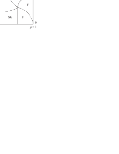
Figure 1: A plausible generic phase diagram of the $\pm J$ model. The system has paramagnetic (P), ferromagnetic (F) and spin glass (SG) phases. The Nishimori line $K=K_{p}$ shown dashed marks a crossover between two regions within the ferromagnetic phase.

The main physical quantities we treat in this paper are the ferromagnetic and spin glass order parameters defined by

$$m=[\langle S_{i}\rangle_{K}],~{}~{}~{}q=[\langle S_{i}\rangle_{K}^{2}],$$ (1)

respectively, with $i$ well interior of the lattice. The inner brackets denote the thermal average with coupling constant $K=J/T$, and the outer square brackets are for the configurational average characterized by the parameter $p$. The spins on the boundary of the lattice under consideration are set to up states to avoid trivial vanishing of the thermal expectation value of the one-point function $\langle S_{i}\rangle_{K}$. It is sufficient to consider a single parameter $q$ as a spin glass order parameter instead of its distribution function $P_{q}(x)$ because replica symmetry breaking is absent when $K=K_{p}\equiv\frac{1}{2}\log(p/(1-p))$ [6, 3], the Nishimori line, on and near which we concentrate ourselves for the moment.

The identity $m=q$ valid when $K=K_{p}$ has long been known [2]. The first of our new results is the following relations:

$$\frac{\partial q}{\partial K}=2\frac{\partial m}{\partial K}$$ (2)

$$\frac{\partial^{2}q}{\partial K^{2}}\geq 2\frac{\partial^{2}m}{\partial K^{2}},$$ (3)

both of which hold under the condition $K=K_{p}$.

The proof is straightforward. As shown in the Appendix, the magnetization is rewritten using gauge transformation as

$$m=[\langle S_{i}\rangle_{K}]=[\langle\sigma_{i}\rangle_{K_{p}}\langle S_{i}\rangle_{K}],$$ (4)

where $\langle\sigma_{i}\rangle_{K_{p}}$ is the thermal average of the Ising spin $\sigma_{i}$ (introduced by the gauge transformation) of the same system as the original $\pm J$ model with effective coupling $K_{p}$. The first and second derivatives of $m$ are then

$$\frac{\partial m}{\partial K}=\left[\langle\sigma_{i}\rangle_{K_{p}}\frac{\partial}{\partial K}\langle S_{i}\rangle_{K}\right],$$ (5)

$$\frac{\partial^{2}m}{\partial K^{2}}=\left[\langle\sigma_{i}\rangle_{K_{p}}\frac{\partial^{2}}{\partial K^{2}}\langle S_{i}\rangle_{K}\right].$$ (6)

The derivatives of the spin glass order parameter are obtained directly from the definition (1):

$$\frac{\partial q}{\partial K}=2\left[\langle S_{i}\rangle_{K}\frac{\partial}{\partial K}\langle S_{i}\rangle_{K}\right],$$ (7)

$$\frac{\partial^{2}q}{\partial K^{2}}=2\left[\langle S_{i}\rangle_{K}\frac{\partial^{2}}{\partial K^{2}}\langle S_{i}\rangle_{K}\right]+2\left[\left(\frac{\partial}{\partial K}\langle S_{i}\rangle_{K}\right)^{2}\right].$$ (8)

The identity $m=q$ for $K=K_{p}$ immediately follows from (4) and (1) because $\langle\sigma_{i}\rangle_{K_{p}}=\langle S_{i}\rangle_{K}$ if $K=K_{p}$. The identity (2) valid for $K=K_{p}$ is also easy to verify from (5) and (7). The inequality (3) is a consequence of (6) and (8).

Similar relations hold for more general correlation functions. Let us define two correlations:

$$C_{ijk\cdots}^{(2l+1)}=[\langle S_{i}S_{j}S_{k}\cdots\rangle_{K}^{2l+1}],~{}~{}~{}C_{ijk\cdots}^{(2l+2)}=[\langle S_{i}S_{j}S_{k}\cdots\rangle_{K}^{2l+2}],$$ (9)

where $l$ is a non-negative integer and $\{i,j,k,\cdots\}$ is an arbitrary set of sites.

This $C_{ijk\cdots}^{(2l+1)}$ satisfies the following identity (see the Appendix)

$$C_{ijk\cdots}^{(2l+1)}=[\langle\sigma_{i}\sigma_{j}\sigma_{k}\cdots\rangle_{K_{p}}\langle S_{i}S_{j}S_{k}\cdots\rangle_{K}^{2l+1}].$$ (10)

Using the fact that $C_{ijk\cdots}^{(2l+2)}$ is gauge invariant, we can prove the following relations at $K=K_{p}$:

$$C_{ijk\cdots}^{(2l+1)}=C_{ijk\cdots}^{(2l+2)},~{}~{}~{}\frac{1}{2l+1}\frac{\partial}{\partial K}C_{ijk\cdots}^{(2l+1)}=\frac{1}{2l+2}\frac{\partial}{\partial K}C_{ijk\cdots}^{(2l+2)}.$$ (11)

No simple relation exists between the second derivatives for general $l$. It is to be noted that equation (11) holds not just in the ferromagnetic phase but in the paramagnetic phase as well whereas equations (2) and (3) are trivial in the paramagnetic phase as both sides vanish identically.

We next discuss our second new result for the order parameters. Let us denote the dependence of the order parameters on the temperature and probability parameter explicitly as $m(K,K_{p})$ and $q(K,K_{p})$. Then it is possible to show that

$$m(K,K_{p})\geq q(K,K_{p})$$

$$\Rightarrow m(K_{p},K_{p})\geq m(K,K_{p})~{}~{}{\rm and}~{}~{}q(K_{p},K_{p})\geq q(K,K_{p})$$ (12)

for any $K$ and $K_{p}$. To prove this, it is useful to write (4) explicitly as

$$m(K,K_{p})=\sum_{k}P(k)\langle\sigma_{i}\rangle_{K_{p}}^{(k)}\langle S_{i}\rangle_{K}^{(k)}=\sum_{k}\sqrt{P(k)}\langle\sigma_{i}\rangle_{K_{p}}^{(k)}\cdot\sqrt{P(k)}\langle S_{i}\rangle_{K}^{(k)},$$ (13)

where $k$ stands for a bond configuration. Let us square both sides of the above equation and apply the Schwarz inequality to obtain

$$m(K,K_{p})^{2} \leq \sum_{k}P(k)(\langle\sigma_{i}\rangle_{K_{p}}^{(k)})^{2}\sum_{k}P(k)(\langle S_{i}\rangle_{K}^{(k)})^{2}$$ (14)

$$= [\langle\sigma_{i}\rangle_{K_{p}}^{2}][\langle S_{i}\rangle_{K}^{2}]$$

$$= q(K_{p},K_{p})q(K,K_{p}).$$

Now, if we assume $m(K,K_{p})\geq q(K,K_{p})$, then $q(K,K_{p})$ on the right hand side can be replaced by $m(K,K_{p})$ to yield

$$m(K,K_{p})^{2}\leq q(K_{p},K_{p})m(K,K_{p}).$$ (15)

Since we are considering the ferromagnetic phase with up-spin boundaries, we have $m(K,K_{p})>0$, and therefore by dividing both sides by $m(K,K_{p})$, we find

$$m(K,K_{p})\leq q(K_{p},K_{p})=m(K_{p},K_{p}).$$ (16)

This is the first half of the result (12).

The second half is proved similarly. From (14) and the assumption $m(K,K_{p})\geq q(K,K_{p})$, we find

$$q(K,K_{p})^{2}\leq q(K_{p},K_{p})q(K,K_{p})$$ (17)

and thus

$$q(K,K_{p})\leq q(K_{p},K_{p}).$$ (18)

A generalization to correlation functions is straightforward. The result is

$$C_{ijk\cdots}^{(2l+1)}(K,K_{p})\geq C_{ijk\cdots}^{(4l+2)}(K,K_{p})$$

$$\Rightarrow C_{ijk\cdots}^{(1)}(K_{p},K_{p})\geq C_{ijk\cdots}^{(2l+1)}(K,K_{p})~{}{\rm and}~{}C_{ijk\cdots}^{(2)}(K_{p},K_{p})\geq C_{ijk\cdots}^{(4l+2)}(K,K_{p}).$$

(19)

To prove these inequalities, we apply the gauge transformation and Schwarz inequality to $C_{ijk\cdots}^{(2l+1)}(K,K_{p})$:

$$C_{ijk\cdots}^{(2l+1)}(K,K_{p})^{2} = [\langle S_{i}S_{j}S_{k}\cdots\rangle_{K}^{2l+1}]^{2}$$ (20)

$$= \left(\sum_{k}\sqrt{P(k)}\langle\sigma_{i}\sigma_{j}\sigma_{k}\cdots\rangle_{K_{p}}^{(k)}\cdot\sqrt{P(k)}\left(\langle S_{i}S_{j}S_{k}\cdots\rangle_{K}^{(k)}\right)^{2l+1}\right)^{2}$$

$$\leq \sum_{k}P(k)\left(\langle\sigma_{i}\sigma_{j}\sigma_{k}\cdots\rangle_{K_{p}}^{(k)}\right)^{2}\sum_{k}P(k)\left(\langle S_{i}S_{j}S_{k}\cdots\rangle_{K}^{(k)}\right)^{4l+2}$$

$$= [\langle\sigma_{i}\sigma_{j}\sigma_{k}\cdots\rangle_{K_{p}}^{2}][\langle S_{i}S_{j}S_{k}\cdots\rangle_{K}^{4l+2}]$$

$$= C_{ijk\cdots}^{(2)}(K_{p},K_{p})C_{ijk\cdots}^{(4l+2)}(K,K_{p}).$$

When $C_{ijk\cdots}^{(2l+1)}(K,K_{p})\geq C_{ijk\cdots}^{(4l+2)}(K,K_{p})$, the second factor on the right hand side of (20) is bounded from above by $C_{ijk\cdots}^{(2l+1)}(K,K_{p})$ to yield

$$C_{ijk\cdots}^{(2l+1)}(K,K_{p})^{2}\leq C_{ijk\cdots}^{(2)}(K_{p},K_{p})C_{ijk\cdots}^{(2l+1)}(K,K_{p}).$$ (21)

Since $C_{ijk\cdots}^{(2l+1)}(K,K_{p})>0$ under the up-spin boundary condition, we have

$$C_{ijk\cdots}^{(2l+1)}(K,K_{p})\leq C_{ijk\cdots}^{(2)}(K_{p},K_{p})=C_{ijk\cdots}^{(1)}(K_{p},K_{p}),$$ (22)

the final inequality being a result of gauge transformation of the kind described in the Appendix. This ends the proof of the first inequality of (19). By replacing the left hand side of (20) with the lower bound $C_{ijk\cdots}^{(4l+2)}(K,K_{p})^{2}$, we arrive at the second relation

$$C_{ijk\cdots}^{(4l+2)}(K,K_{p})\leq C_{ijk\cdots}^{(2)}(K_{p},K_{p}).$$ (23)

It is possible to apply similar arguments to the other models of spin glasses with gauge symmetry including the random Ising model with Gaussian-distributed interactions and $XY$ gauge glass [3, 8]. The physical significance of the results obtained in this section will be discussed in the next section.

3 Discussions

An immediate consequence of (2) is that the derivatives of $q$ and $m$ have the same sign when $K=K_{p}$. It is forbidden that, for example, the spin glass order parameter $q$ increases whereas the ferromagnetic order parameter $m$ decreases as depicted in figure 2.

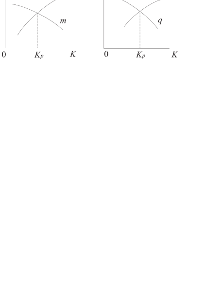
Figure 2: It is forbidden that the derivatives of $m$ and $q$ have different signs at $K=K_{p}$ as shown in this figure.

In the plausible case that $\partial q/\partial K>0$, it follows from (2) that $q$ increases twice as rapidly as $m$ does as the temperature is lowered (see figure 3 (left)).

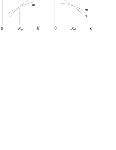
Figure 3: The spin glass order parameter increases twice as rapidly as the ferromagnetic order parameter around $K=K_{p}$ if these quantities are increasing functions of $K$ (left). The opposite possibility is shown on the right.

It naturally follows that $q$ is larger than $m$ at least slightly below the Nishimori line $(K>K_{p})$ and the opposite inequality $m>q$ holds when $K<K_{p}$. This is the most natural case as discussed in the introduction: The ferromagnetic ordering is dominant $(m>q)$ above the Nishimori line ($K<K_{p}$) and quenched-disorder-driven random ordering proliferates in the sense $q>m$ below the same line ($K>K_{p}$). The point is that we have reduced the inequality $q>m$ for $K>K_{p}$ to an intuitively natural relation $\partial q/\partial K>0$ at $K=K_{p}$ (although we still do not have a rigorous proof of the latter.)

If the opposite inequality $\partial q/\partial K<0$ holds at $K=K_{p}$, the order parameters behave as depicted in figure 3 (right). We cannot exclude this possibility from the present argument, but it seems quite unlikely that both order parameters $q$ and $m$ decrease with temperature decrease on and around the line $K=K_{p}$ which runs through the central part of the ferromagnetic phase as seen in figure 1. If there exists a reentrant transition (below which $m$ vanishes but $q$ can stay finite), only $m$ may decrease toward such a transition temperature from above unlike figure 3 (right). Although we believe that such a situation is not plausible to exist [9], it would happen at very low temperatures if it does at all, not around the line $K=K_{p}$ which runs through relatively high temperature parts of the ferromagnetic phase.

The final possibility is that the derivatives in (2) vanish. Again, both derivatives should vanish, not just one of them. The inequality for the second derivative (3) does not tell much about the behaviour of $m$ and $q$ around $K=K_{p}$.

It is instructive to remember in this connection that the average sign of local magnetization reaches its maximum at $K=K_{p}$ as a function of $K$ (or the temperature) [5]

$$M(K,K_{p})\equiv[{\rm sgn}\langle S_{i}\rangle_{K}]\leq M(K_{p},K_{p}).$$ (24)

This means that the number of up spins under up-spin boundaries becomes maximum at $K=K_{p}$ as a function of $K$. Although this relation (24) can be proved for an arbitrary $K$ by the gauge theory [5], it is useful to check it by taking the derivative of (24) (as we did for $m$ and $q$):

$$\frac{\partial M}{\partial K}=\left[\frac{\partial}{\partial K}{\rm sgn}\langle S_{i}\rangle_{K}\right]=2\left[\delta(\langle S_{i}\rangle_{K})\frac{\partial}{\partial K}\langle S_{i}\rangle_{K}\right]=2\left[\langle\sigma_{i}\rangle_{K_{p}}\delta(\langle S_{i}\rangle_{K})\frac{\partial}{\partial K}\langle S_{i}\rangle_{K}\right]=0,$$ (25)

the last equality being valid for $K=K_{p}$. Equation (25) implies that the effects of spins with positive temperature derivative ($\partial\langle S_{i}\rangle_{K}/\partial K>0$) just match those of negative temperature derivative ($\partial\langle S_{i}\rangle_{K}/\partial K<0$) at $K=K_{p}$ if we concentrate ourselves on the spins with vanishing local magnetization $\delta(\langle S_{i}\rangle_{K})$. Thus, at $K=K_{p}$, some spins change its local magnetization from positive value to negative value whereas essentially the same number of spins change the sign of local magnetization in the opposite way. It should be noted, however, that this observation does not necessarily mean vanishing derivatives of the ferromagnetic and spin glass order parameters at $K=K_{p}$, that is, $\partial m/\partial K$ and $\partial q/\partial K$ are in general not vanishing at $K=K_{p}$: The absolute value of local magnetization $|\langle S_{i}\rangle_{K}|$, which is ignored in $M(K)$, at sites with $\langle S_{i}\rangle_{K}>0$ may grow more rapidly than at sites with $\langle S_{i}\rangle_{K}<0$ as $K$ decreases, compensating for the decrease in the number of up spins below $K=K_{p}$, leading to a positive derivative $\partial m/\partial K>0$.

The present argument does not apply in the paramagnetic phase where the order parameters $m$ and $q$ vanish. However, the relation (11) for correlation functions, the two-point functions $C_{ij}^{(2l+1)}(K,K_{p})$ and $C_{ij}^{(2l+2)}(K,K_{p})$ in particular, suggests that $C_{ij}^{(2l+1)}(K,K_{p})>C_{ij}^{(2l+2)}(K,K_{p})$ if $K<K_{p}$ and $C_{ij}^{(2l+1)}(K,K_{p})<C_{ij}^{(2l+2)}(K,K_{p})$ if $K>K_{p}$. This means that the ferromagnetic correlation length $\xi_{m}$ (defined by $C_{0r}^{(1)}\approx\exp(-r/\xi_{m}),r\gg 1$) is larger than the spin glass correlation length $\xi_{q}$ (defined by $C_{0r}^{(2)}\approx\exp(-r/\xi_{q}),r\gg 1$) for $K<K_{p}$ (above the Nishimori line) whereas the opposite inequality holds below the line.

Very similar conclusions follow from the result (12). The relation between $m$ and $q$ shown in figure 2 violates these inequalities because, in the temperature range where $m(K,K_{p})$ exceeds $q(K,K_{p})$, $m(K,K_{p})$ is seen to be larger than its value at $K=K_{p}$. The cases given in figure 3 are compatible with the present inequalities: If $m(K,K_{p})>q(K,K_{p})$, then $m(K,K_{p})$ is smaller than $m(K_{p},K_{p})$. An advantage of the present inequalities (12) over the relation (2) is that we can analyze the behaviour of order parameters well away from the Nishimori line, that is, $K$ can be much larger or smaller than $K_{p}$. A weak point is that quantitative relations for the increase/decrease rates are not given unlike (2). Another problem to remember concerning (12) is that we may not be able to describe the system only in terms of $m$ and $q$ at very low temperatures if replica symmetry breaking exists as it is the case in the Sherrington-Kirkpartrick model [10].

The analysis presented above strongly indicates that the Nishimori line $K=K_{p}$ marks a crossover between the purely ferromagnetically-ordered region and disorder-dominated region within the ferromagnetic phase. This observation is consistent also with renormalization group analyses: The low-temperature region is controlled by a fixed point at $T=0$ with finite disorder ($p<1$) whereas the high-temperature region is described by a different fixed point representative of the critical curve above the multicritical point [11, 12].

An important future direction of investigation is a rigorous proof of the relation $\partial m/\partial K>0$ at $K=K_{p}$, which needs additional ideas.

Appendix

In this Appendix we drive equations (4) and (10) following references [2] and [3]. The ferromagnetic order parameter is defined by

$$m=[\langle S_{i}\rangle_{K}]=\frac{1}{(2\cosh K_{p})^{N_{B}}}\sum_{\{\tau_{ij}=\pm 1\}}\exp(K_{p}\sum_{\langle ij\rangle}\tau_{ij})\frac{\sum_{\{S\}}S_{i}\exp(K\sum_{\langle ij\rangle}\tau_{ij}S_{i}S_{j})}{\sum_{\{S\}}\exp(K\sum_{\langle ij\rangle}\tau_{ij}S_{i}S_{j})}.$$ (26)

Here $\tau_{ij}$ is the sign of $J_{ij}$ ($\tau_{ij}=J_{ij}/|J_{ij}|=\pm 1$), the sums in the exponents run over all pairs of sites on the lattice under consideration, and $N_{B}$ is the total number of bonds. The factor $\exp(K_{p}\tau_{ij})/2\cosh K_{p}$ gives the probability weight of configurational average of the $\pm J$ model since this quantity equals $p$ for $\tau_{ij}=1$ and $1-p$ for $\tau_{ij}=-1$ as can be verified from the definition $K_{p}=\frac{1}{2}\log(p/(1-p))$. Spins on the boundary are all up.

Let us apply a gauge transformation

$$S_{i}\to S_{i}\sigma_{i},~{}~{}~{}\tau_{ij}\to\tau_{ij}\sigma_{i}\sigma_{j}$$ (27)

to all sites, where $\sigma_{i}$ is a gauge variable fixed either to $1$ or $-1$ arbitrarily at each site ($+1$ on the boundary). The Hamiltonian in the exponents of (26) is invariant under this gauge transformation. Since the gauge transformation is just a re-definition of running variables in (26), it does not affect the value of the right hand side, and we have

$$m=\frac{1}{(2\cosh K_{p})^{N_{B}}}\sum_{\{\tau_{ij}\}}\exp(K_{p}\sum_{\langle ij\rangle}\tau_{ij}\sigma_{i}\sigma_{j})\frac{\sigma_{i}\sum_{\{S\}}S_{i}\exp(K\sum_{\langle ij\rangle}\tau_{ij}S_{i}S_{j})}{\sum_{\{S\}}\exp(K\sum_{\langle ij\rangle}\tau_{ij}S_{i}S_{j})}.$$ (28)

As both sides of this equation are independent of the choice of the values of $\{\sigma_{i}\}$, we may sum the right hand side over all possible values of $\{\sigma_{i}\}$ and divide the result by $2^{N}$, where $N$ is the total number of sites, to find

$$m=\frac{1}{2^{N}(2\cosh K_{p})^{N_{B}}}\sum_{\{\tau_{ij}\}}\sum_{\{\sigma_{i}\}}\sigma_{i}\exp(K_{p}\sum_{\langle ij\rangle}\tau_{ij}\sigma_{i}\sigma_{j})\langle S_{i}\rangle_{K}.$$ (29)

By inserting the identity $1=Z(K_{p},\{\tau_{ij}\})/Z(K_{p},\{\tau_{ij}\})$ just in front of the sum over $\{\sigma_{i}\}$ in the summand, we obtain

$$m=\frac{1}{2^{N}(2\cosh K_{p})^{N_{B}}}\sum_{\{\tau_{ij}\}}\sum_{\{\sigma_{i}\}}\exp(K_{p}\sum_{\langle ij\rangle}\tau_{ij}\sigma_{i}\sigma_{j})\frac{\sum_{\{\sigma_{i}\}}\sigma_{i}\exp(K_{p}\sum_{\langle ij\rangle}\tau_{ij}\sigma_{i}\sigma_{j})}{\sum_{\{\sigma_{i}\}}\exp(K_{p}\sum_{\langle ij\rangle}\tau_{ij}\sigma_{i}\sigma_{j})}\langle S_{i}\rangle_{K}$$ (30)

$$\hbox to0.0pt{\hss${}={}$}\frac{1}{2^{N}(2\cosh K_{p})^{N_{B}}}\sum_{\{\tau_{ij}\}}\sum_{\{\sigma_{i}\}}\exp(K_{p}\sum_{\langle ij\rangle}\tau_{ij}\sigma_{i}\sigma_{j})\,\langle\sigma_{i}\rangle_{K_{p}}\langle S_{i}\rangle_{K}$$ (31)

$$\hbox to0.0pt{\hss${}={}$}\frac{1}{(2\cosh K_{p})^{N_{B}}}\sum_{\{\tau_{ij}\}}\exp(K_{p}\sum_{\langle ij\rangle}\tau_{ij})\langle\sigma_{i}\rangle_{K_{p}}\langle S_{i}\rangle_{K}.$$ (32)

The last line (32) can be confirmed by applying the gauge transformation to (32) and using the same argument as above with gauge invariance of the product $\langle\sigma_{i}\rangle_{K_{p}}\langle S_{i}\rangle_{K}$ in mind to derive (31). Equation (32) is exactly the definition of the right hand side of (4), which completes the proof. A similar argument leads to (10).

References

References

• [1] Young A P (Ed.) 1998 Spin Glasses and Random Fields (Singapore: World Scientific)
• [2] Nishimori H 1981 Prog. Theor. Phys. 66 1169
• [3] Nishimori H 2001 Statistical Physics of Spin Glasses and Information Processing: An Introduction (Oxford: Oxford University Press)
• [4] Nishimori H and Sollich P 2000 J. Phys. Soc. Japan69 Suppl. A 160
• [5] Nishimori H 1993 J. Phys. Soc. Japan62 2973
• [6] Nishimori H and Sherrington D 2001 in Disordered and Complex Systems (Eds. Sollich P, Coolen A C C, Hughston L P and Streater R F) p. 67 (Melville: AIP)
• [7] Sherrington D and Kirkpatrick S 1975 Phys. Rev. Lett.35 1792
• [8] Ozeki Y and Nishimori H 1993 J. Phys. A: Math. Gen.26 3399
• [9] Nishimori H 1986 J. Phys. Soc. Japan55 3305
• [10] de Almeida J R L and Thouless D J 1978 J. Phys. A: Math. Gen.11 983
• [11] Le Doussal P and Harris A B 1989 Phys. Rev.B 40 9249
• [12] Hukushima K 2000 J. Phys. Soc. Japan69 631