Comments on Sweeny and Gliozzi dynamics for simulations of Potts models in the Fortuin-Kasteleyn representation

Abstract

We compare the correlation times of the Sweeny and Gliozzi dynamics for two-dimensional Ising and three-state Potts models, and the three-dimensional Ising model for the simulations in the percolation representation. The results are also compared with Swendsen-Wang and Wolff cluster dynamics. It is found that Sweeny and Gliozzi dynamics have essentially the same dynamical critical behavior. Contrary to Gliozzi’s claim (cond-mat/0201285), the Gliozzi dynamics has critical slowing down comparable to that of other cluster methods. For the two-dimensional Ising model, both Sweeny and Gliozzi dynamics give good fits to logarithmic size dependences; for two-dimensional three-state Potts model, their dynamical critical exponent $z$ is $0.49\pm 0.01$; the three-dimensional Ising model has $z=0.37\pm 0.02$.

Cluster algorithms have played an interesting role in statistical physics, both for their importance in constructing efficient computational algorithms and their unusual dynamical properties. Very recently, Gliozzi has introduced a new cluster algorithm, which he claims to be free of critical slowing down gliozzi .  Since an understanding of the dynamics at the critical temperature is central to both dynamic universality classes and computational efficiency, we have made a comparison of the four main cluster methods for Potts models due to Sweeny sweeny , Swendsen and Wang swendsen-wang , Wolff wolff , and Gliozzi gliozzi .

In 1983 Sweeny sweeny simulated the Potts model wu directly in the Fortuin-Kasteleyn representation FK , given by the probability distribution of percolation bond configuration $\Gamma$,

$$P(\Gamma)\propto\left({\frac{p}{1-p}}\right)^{b}q^{N_{c}},$$ (1)

where $p=1-\exp\bigl{(}-J/(kT)\bigr{)}$, $J$ is coupling constant in the Potts model, $k$ is Boltzmann constant, and $T$ is temperature; $b$ is the number of bonds present on the (hypercubic) lattice, and $N_{c}$ is the number of clusters of the percolation configuration.

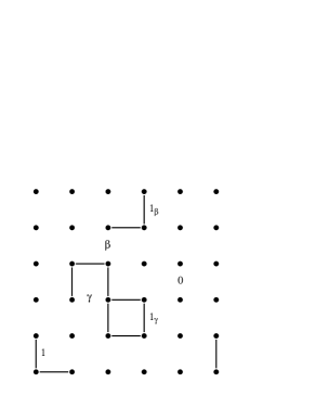
Figure 1: Different types of links: $1$ (occupied bond), $0$ (absence of a bond), $\beta$ (unoccupied link that bridges two clusters), $\gamma$ (unoccupied link that spans the same cluster), $1_{\beta}$ (bond, removing of which breaks the cluster), $1_{\gamma}$ (bond, removing of which does not break the cluster).

Sweeny used a heat-bath rate of “flipping” the links from occupied to empty or vice versa. Consider a particular link. We define the state $1$ to mean a presence of a bond, $0$ for absence of a bond, $\beta$ for unoccupied link such that the two nearest neighbor sites are on different clusters, and $\gamma$ for unoccupied link that spans the same cluster, see Fig. 1. In addition, we define $1_{\beta}$ to be an occupied bond, the removal of which leads to $\beta$, and similarly $1_{\gamma}$ is an occupied bond, the removal of which leads to $\gamma$.   Finally, a dot $\cdot$ represents an arbitrary state (0 or 1). Assuming a link is picked up at random, the transition rate for Sweeny’s dynamics is

$$w(\cdot\rightarrow 1_{\gamma})=p, \!\!\!\!w(\cdot\rightarrow\gamma)=1-p,$$ (2a)

$$w(\cdot\!\rightarrow\!1_{\beta})={\frac{p}{(1\!-\!p)q\!+\!p}}, \!\!\!\!w(\cdot\!\rightarrow\!\beta)={\frac{(1\!-\!p)q}{(1\!-\!p)q\!+\!p}}.$$ (2b)

Note that the transition probabilities do not depend on the initial state, as it is generally the case for heat-bath algorithms.

Gliozzi also worked in the Fortuin-Kasteleyn representation FK and proposed a variation on the flip rate gliozzi that is only slightly different from Sweeny’s:

$$w(1\rightarrow 1)=p, w(1\rightarrow 0)=1-p,$$ (3a)

$$w(\gamma\rightarrow 1)=p, w(\gamma\rightarrow 0)=1-p,$$ (3b)

$$w(\beta\rightarrow 1)=p/q, w(\beta\rightarrow 0)=1-p/q.$$ (3c)

One can easily show that both of algorithms satisfy detailed balance with respect to the equilibrium distribution, Eq. (1). Both Sweeny and Gliozzi’s rates are applicable to model with real positive $q$ (not just integer values), although Gliozzi’s rate has the restriction that $p/q\leq 1$. We also note that Chayes and Machta proposed a cluster algorithm for noninteger $q$ that takes $O(L^{d})$ operations per sweep chayes .

A key implementation issue in both algorithms is the determination of whether two sites belong to the same cluster. For two dimensions, Sweeny devised a very efficient method based on the special topology. In three and higher dimensions, one has to contend with the shortcomings that a move takes an amount of CPU time proportional to the typical size of the clusters.

To separate the issues of the intrinsic dynamics of the transition rates from the efficiency of the numerical implementation, we present results for the correlation times of both Sweeny and Gliozzi dynamics, measured in Monte Carlo sweeps regardless of the actual computer time for a particular implementation. We also compare them in the same way with Swendsen-Wang swendsen-wang and Wolff wolff cluster dynamics.

We consider the integrated correlation time, which is directly relevant to the magnitude of statistical errors MK-Binder . Instead of the usual method of computing the autocorrelation function for, say, energy,

$$f(t)={\frac{\langle E(0)E(t)\rangle-\langle E(0)\rangle^{2}}{\langle E(0)^{2}\rangle-\langle E(0)\rangle^{2}}},$$ (4)

a totally equivalent way is to compute the variance of $M$ consecutive terms of the sum of energies,

$$E_{M}={\frac{1}{M}}\sum_{t=1}^{M}E(t).$$ (5)

We have for the variance landau-binder

$$\mathrm{var}(E_{M})={\frac{\tau_{M}\,\mathrm{var}(E_{1})}{M}}.$$ (6)

A straightforward variance estimator, i.e., the squared mean minus the sample mean squared, is used. The usual correlation time $\tau$ is the limit of $M$ going to infinity, and is related to the correlation function by

$$\tau=\lim_{M\rightarrow\infty}\tau_{M}=\sum_{t=-\infty}^{\infty}f(t).$$ (7)

Kikuchi et al okabe have used a similar method to extract exponential correlation times. Other conventions for specifying the correlation time are in use. For example, Müller-Krumbhaar and Binder MK-Binder call $\tau^{\prime}$ the correlation time, where $\tau=1+2\tau^{\prime}$, and Baillie and Coddington baillie use the definition $\tau^{\prime\prime}=\tau/2$.

Figure 2: $\tau_{M}$ versus $1/M$ for the two-dimensional Ising model with Gliozzi dynamics on a $32\times 32$ lattice, with $8\times 10^{6}$ Monte Carlo sweeps. The straight is an error weighted least-square fit. The intercept gives the correlation time $\tau=6.53\pm 0.01$.

The truncated sum converges to its limit according to $1/M$. Thus we obtain the limit with a plot of $\tau_{M}$ versus $1/M$, as shown in Figure 2. The method appears excellent for dynamics with relatively small values of $\tau$. When $\tau$ is large, we have to go to much bigger values of $M$, where the noise can dominate the signal, rendering the method less useful.

Table 1: Correlation time $\tau$ for Sweeny and Gliozzi dynamics at various system sizes. The number in parentheses is standard error at the last digits.

$L$	Sweeny rate	Gliozzi rate
2D Ising
2	2.6121(3)	2.9414(4)
4	3.3280(3)	3.8722(7)
8	4.006(2)	4.738(1)
16	4.688(5)	5.607(5)
32	5.46(2)	6.51(3)
64	6.21(3)	7.54(5)
2D $q=3$ Potts
2	3.0736(2)	3.8111(4)
4	4.5375(8)	5.9245(5)
8	6.424(2)	8.604(3)
16	9.06(2)	12.18(1)
32	12.56(5)	17.10(5)
64	17.5(3)	24.0(2)
3D Ising
2	3.0242(3)	3.3456(4)
4	4.254(2)	4.814(16)
8	5.594(8)	6.375(8)
16	7.1(1)	8.0(2)
32	9.0(5)	11.4(10)

Figure 3: Correlation times $\tau$ versus lattice linear dimension $L$ on a semi-logarithmic scale for the two-dimensional Ising model at $T_{c}$. The circles are for Sweeny, squares for Gliozzi, diamonds for Swendsen-Wang, and triangles for Wolff dynamics. Straight lines are fits to asymptotic slopes at large $L$. The Swendsen-Wang data are from ref. WangMCQMC and Wolff data are from ref. baillie .

Figure 4: Same as Fig. 3, but on a double logarithmic scale for the two-dimensional three-state Potts model at $T_{c}$. The number on the line indicates the slope of the line. The Swendsen-Wang and Wolff data are from ref. baillie .

Figure 5: Correlation times $\tau$ versus lattice linear dimension $L$ on a double logarithmic scale for the three-dimensional Ising model at $T_{c}$ of Sweeny (circles), Gliozzi (squares), Swendsen-Wang (diamonds), and Wolff (triangles) dynamics. The number on the straight line indicates the slope of the line.

We performed our simulations at the critical temperature $kT_{c}(q)/J=1/\ln(\sqrt{q}+1)$ in two dimensions, and at $J/(kT_{c})=0.221657$ for the three-dimensional Ising model landau . For each data point, we have spent about two to four weeks of CPU time on 1GHz Pentium PCs. For the Sweeny and Gliozzi dynamics, a unit of time $t$ for a lattice linear dimension $L$ in $d$ dimensions is $dL^{d}$ moves with bond selected at random. We note that Gliozzi used a sequential sweep of the bonds, which gives correlation time that is smaller by a factor about 0.6. The correlation time data are given in Table 1.

Fig. 3 contains a semilogarithmic plot of $\tau$ versus $L$ for the four algorithms: Sweeny, Gliozzi, Swendsen-Wang, and Wolff. It is remarkable that Gliozzi dynamics and to some extent Sweeny is perfectly logarithmic in size down to $2\times 2$ lattice. For both Swendsen-Wang and Wolff, some curvature can be seen in this plot, and the data can also be fitted with a small exponent of 0.25 baillie as well. We consider it still to be an open question for Swendsen-Wang and Wolff dynamics whether the correlation times depend on lattice sizes as a small power or logarithmically heermann .

In Fig. 4, results for the two-dimensional, three-state Potts model are presented. The straight lines in these log-log plots show good power-law dependence for all algorithms. The data show an interesting possibility that Sweeny and Gliozzi belong to a different dynamical universality class from Swendsen-Wang. Linear least-squares fits give the dynamical critical exponent $z=0.56\pm 0.01$ for Swendsen-Wang and $0.58\pm 0.01$ for Wolff, with lower values of $0.48\pm 0.01$ for Sweeny and $0.49\pm 0.01$ for Gliozzi dynamics. The differences are statistically significant.

Figure 5 is for the three-dimensional Ising model. Again we see similar behavior, although the data are less accurate comparing to that of two dimensions. Sweeny and Gliozzi dynamics have approximately the same dynamical critical exponent of $0.37\pm 0.02$, while that of the Swendsen-Wang is larger at about $0.5$. Wolff single cluster algorithm gives remarkably small correlation times and a small exponent of $0.29$ wolff3D . The Swendsen-Wang data show some curvature and might approach the same asymptotic value for large lattices.

In summary, we have computed the correlation times for cluster algorithms. It is clear that Sweeny and Gliozzi have the same dynamics. In all cases studied here, the Sweeny rate is actually better than Gliozzi’s. Both rates reduce critical slowing down, but not completely eliminate it. Both Sweeny and Gliozzi dynamics seem to have somewhat smaller dynamical critical exponents than Swendsen-Wang when measured in units of Monte Carlo sweeps, as we have done in this paper.

J.-S. W. acknowledges the hospitality of the Departments of Physics of Carnegie Mellon University and Tokyo Metropolitan University, where part of the work was done during a sabbatical leave. He also thanks Y. Okabe for discussion.

References

- (1) F. Gliozzi, cond-mat/0201285.
- (2) M. Sweeny, Phys. Rev. B 27, 4445 (1983).
- (3) R. H. Swendsen and J.-S. Wang, Phys. Rev. Lett. 58, 86 (1987).
- (4) U. Wolff, Phys. Rev. Lett. 62, 361 (1989); Nucl. Phys. B322, 759 (1989).
- (5) F. Y. Wu, Rev. Mod. Phys. 54, 235 (1982).
- (6) P. W. Kasteleyn and C. M. Fortuin, J. Phys. Soc. Jpn Suppl. 26, 11 (1969); C. M. Fortuin and P. W. Kasteleyn, Physica 57, 536 (1972).
- (7) L. Chayes and J. Machta, Physica A 254, 477 (1998).
- (8) H. Müller-Krumbhaar and K. Binder, J. Stat. Phys. 8, 1 (1973).
- (9) See, e.g., D. P. Landau and K. Binder, A Guide to Monte Carlo Simulations in Statistical Physics, pp. 91–93 (Cambridge University Press, 2000).
- (10) M. Kikuchi, N. Ito, and Y. Okabe, in Computer Simulation Studies in Condensed-Matter Physics VII, p.44, Eds. D. P. Landau, K. K. Mon, H.-B. Schüttler, (Springer, Berlin, 1994).
- (11) C. F. Baillie and P. D. Coddington, Phys. Rev. B, 43, 10617 (1991).
- (12) J.-S. Wang, cond-mat/0103318.
- (13) A. M. Ferrenberg and D. P. Landau, Phys. Rev. B, 44, 5081 (1991).
- (14) D. W. Heermann and A. N. Burkitt, Physica A 162, 210 (1990).
- (15) U. Wolff, Phys. Lett. B 228, 379 (1989).