Time-resolved dynamics of electron wave packets in chaotic and regular quantum billiards with leads

Abstract

We perform numerical studies of the wave packet propagation through open quantum billiards whose classical counterparts exhibit regular and chaotic dynamics. We show that for $t\lesssim\tau_{H}$ ($\tau_{H}$ being the Heisenberg time), the features in the transmitted and reflected currents are directly related to specific classical trajectories connecting the billiard leads. In contrast, the long-time asymptotics of the wave packet dynamics is qualitatively different for classical and quantum billiards. In particularly, the decay of the quantum system obeys a power law that depends on the number of decay channels, and is not sensitive to the nature of classical dynamics (chaotic or regular).

Low-dimensional nanometer-scaled semiconductor structures, quantum dots (sometimes called the quantum electron billiards) represent artificial man-made systems which are well suited to study different aspects of quantum-mechanical scattering Marcus_Andy . A majority of studies of electron transport in such systems have been mainly focused on the stationary electron dynamics. In recent years, however, interest in temporal aspect of quantum scattering has been renewed Heller1 . This includes e.g., studies of the time delay distributions Fyodorov and correlation decay in quantum billiards and related systems Ben . Furthermore, many core starting points in the description of the stationary scattering rely heavily on the properties of the system in the time domain. In particular, the semiclassical approach exploits the difference between the classical escape rate from the cavities with chaotic and regular (or mixed) dynamics (exponentially fast $e^{-\gamma t}$ for the former vs. power-law $t^{-\xi}$ for the later Bauer ). This difference in the classical dynamics translates into the the difference in observed transport properties (statistics of the fluctuations Smilansky ; Jalabert ; Ker , a shape of the weak localization Baranger , etc.).

On the other hand, the quantum mechanical (QM) approaches predict qualitatively different, universal power-law escape rate from the cavity Muller ,

$$d\,P(t)/\,d\,t\ \sim\ t^{-\beta\frac{M}{2}-1},$$ (1)

where $P(t)$ is the survival probability, $M$ is the number of decay channels and $\beta=1\ (2)$ for the system with (without) time-reversal invariance . The non-exponential decay of a quantum system with chaotic classical dynamics has been indirectly demonstrated Alt in a microwave stadium billiard.

The QM power-law delay time for the chaotic cavity is expected to deviate from the semi-classical (SC) decay at times of the order of the Heisenberg time $\tau_{H}=\hbar/\Delta,\ \Delta$ being the mean level spacing of the cavity Lewenkopf . At the same time, the difference in the classical decay of the chaotic and regular/mixed cavities often becomes discernible only after many bounces at the times which often exceed $\tau_{H}$ TB2 . Nevertheless, the SC predictions are widely used in experiment to distinguish between the chaotic and regular/mixed dynamics in quantum billiards Marcus_Andy . Is it thus possible to reconcile the SC and QM approaches, or should some of the SC predictions be used with certain caution or even be revised? Does the long-time decay asymptotics of the quantum systems depend on the underlying classical dynamics (chaotic or regular)? Motivated by these questions we, in this paper, perform direct quantum mechanical calculations of the passage of electron wave packets through two-dimensional electron billiards.

To the best of our knowledge, all of the studies of wave packets dynamics in open systems presented so far, have been mostly restricted to (a) quantum limit where a characteristic size of the system $L$ was of the order of the average wavelength of the wave packet $\langle\lambda\rangle$ and (b) to an initial stage of the wave packet evolution $t\lesssim 1$ (where $t$ is in units of the traversal time). The time-dependent solution of the Schrödinger equation was typically obtained on the basis of direct schemes approximating the exponential time propagator time . With such methods the task of tracing the long-time evolution of a wave packet in a realistic quantum dot would be forbiddingly expensive in terms of both computing power and memory. In the present paper we thus implement a spectral method based on the Green function technique Hauge , which allows us (a) to reach a semi-classical regime $\langle\lambda\rangle\gg L$ and (b) to approach a long-time asymptotics $t\gg 1$ corresponding to $10^{4}-10^{5}$ bounces of a classical particle in a billiard. We found that during the initial phase $t\lesssim\tau_{H}$ (which in our case corresponds to $\sim 10-20$ classical bounces in a billiard), the QM decay closely follows the classical one, such that all the features in the QM current leaking out of the billiard can be explained in terms of geometry-specific classical trajectories between the leads. When $t\gtrsim\tau_{H}$, the QM dynamics starts to deviate from the classical one, with the decay rate obeying a power law that depends on the number of decay channels only, irrespective of the nature of classical dynamics (chaotic or regular). We thus conclude that quantum mechanics smears out the difference between classically chaotic and regular motion.

We have studied the temporal evolution of wave packets in square, Sinai, and stadium billiards of various shapes. All of them exhibit similar features and we thus present here the results for two representative geometries, a square (which is classically regular) and a quarter-stadium (which is classically chaotic), see Fig. 1. The billiards are connected to two semi-infinite leads that can support one or more propagating modes. Magnetic field is restricted to zero. We assume a hard wall confinement both in the leads and in the interior of billiards.

Figure 1: A square and a quarter-stadium shaped billiard connected to semi-infinite leads; $L=R,L/w=8$. The half-width of the wave packet $\sigma=0.4L$; at $t=0$ the wave packet is distinct from zero in the interval of $3L$. The average wavelength of the wave packet $\langle\lambda\rangle=2\pi/\langle k\rangle=0.8w$.

Dynamics of the wave packet is governed by the time-dependent Schrödinger equation

$$\left(i\hbar\frac{\partial}{\partial t}-H\right)|\psi(t)\rangle=0,$$ (2)

where $H$ is the Hamiltonian operator and $|\psi(t)\rangle$ is the wave function. To study the time evolution of the initial state we follow Støvneng and Hauge Hauge and perform the Laplace transform of Eq. (2) followed by the integration by parts. Changing variables in the Mellin inversion integral we obtain

$$|\psi(t)\rangle=\frac{i}{2\pi}\int^{\infty+i0}_{-\infty+i0}dz\,G(z)|\psi(0)\rangle e^{-izt/\hbar},$$ (3)

where we have introduced the Green function operator $G(z)=(z-H)^{-1}$ and taken into account that all the poles of the Green function lie in the lower $z$-plane. With the help of Eq. (3), the calculation of the temporal evolution of the initial state is effectively reduced to the computation of the Green function of the Hamiltonian operator $H$ in the energy domain. To compute the Green function we discretize the system under consideration, introduce a standard tight-binding Hamiltonian and make use of the modified recursive Green-function technique described in details in Z .

Let us consider a minimum-uncertainty wave packet of the average energy $E$ which enters a billiard from the left lead in one of the transverse modes $\alpha$. We thus write the initial state in the left lead at $t=0$ in the form

$$|\psi_{\alpha}(0)\rangle = \sum_{mn}\phi_{m}^{\alpha}f^{n}_{\alpha}|mn\rangle,$$ (4)

$$\phi_{m}^{\alpha} = \frac{1}{(2\pi)^{1/4}\sqrt{\sigma}}e^{-\frac{(m-m_{0})^{2}}{4\sigma^{2}}+ik_{\parallel}^{\alpha}m}$$ (5)

where $w$ is the width of the leads (measured in units of a lattice constant $a$), $f^{n}_{\alpha}=\sqrt{2/w}\sin(\pi\alpha n/w)$ is the eigenfunction of the transverse motion; $\langle k\rangle=2\pi/\langle\lambda\rangle=\sqrt{E/u}$ is the average wave vector (in units of $a^{-1}$), where $u=\hbar^{2}/2m^{*}a^{2}$ and $m^{*}$ being the effective mass; $\langle k\rangle^{2}={k_{\parallel}^{\alpha}}^{2}+{k_{\perp}^{\alpha}}^{2}$, $k_{\perp}^{\alpha}=\pi\alpha/w$, with $k_{\parallel}^{\alpha}$ and $k_{\perp}^{\alpha}$ being the longitudinal and transverse wave vectors respectively. The matrix element $\langle m,n|\psi\rangle$ defines the probability amplitude to find the electron on the site ($m,n$). After the wave packet enters the billiard, it will leak out through both of the leads in all the available modes $\beta$. The wave function in e.g. the right lead can then be written in the form

$$|\psi_{\alpha}(t)\rangle=\sum_{m\beta}c_{\beta\alpha}^{m}(t)|m\beta\rangle,$$ (6)

where $|m,\alpha\rangle=\sum_{n}f_{\alpha}^{m}|mn\rangle$; $c_{\beta\alpha}^{m}$ gives a probability to find a particle on the slice $m$ in the transverse mode $\beta$, provided the initial state enters the billiard in the mode $\alpha$. Discretizing a standard expression for the quantum-mechanical current, $j(x,y)=i\hbar/2m^{*}\left(\psi\nabla\psi^{*}-\psi^{*}\nabla\psi\right)$ we, using Eq. (6), obtain the following expression for the total current $J=\int\,dy\,j(x,y)$ through the slice $m$ in the leads expressed via coefficients $c_{\beta\alpha}^{m}(t)$

$$J=\frac{i\hbar}{m^{*}a}\sum_{\beta}\left[c_{\beta\alpha}^{m}\left({c_{\beta\alpha}^{m+1}}^{*}-{c_{\beta\alpha}^{m-1}}^{*}\right)-\text{c.c.}\right].$$ (7)

Note that the quantum-mechanical current is related to the survival probability in the billiard Eq. (1) by the obvious relation

$$d\,P(t)/\,d\,t\,=-J_{l}(t)-J_{r}(t),$$ (8)

where $J_{l}(t)$ and $J_{r}(t)$ stand for the currents flowing into the left and right leads respectively. Note that the function $J_{l}(t)+J_{r}(t)$ has a meaning of the distribution of the time delays in the billiard Fyodorov We calculate coefficients ${c_{\beta\alpha}^{m+1}}$ in Eq. (7) by computing a matrix element $\langle m\beta|\psi\rangle$ using Eqs. (3)-(6)

$$c_{\beta\alpha}^{m}(t)=\frac{i}{2\pi}\int^{\infty+i0}_{-\infty+i0}dz\,\sum_{m^{\prime}}G_{\beta\alpha}^{mm^{\prime}}(z)\phi_{m}^{\alpha}e^{-izt/\hbar},$$ (9)

where $G_{\beta\alpha}^{mm^{\prime}}(z)$ stands for the matrix element $\langle m\beta|G(z)|m^{\prime}\alpha\rangle$ of the Green function of the whole system (billiard and semi-infinite leads).

A special care has been taken to ensure the reliability of the results of the numerical simulations. This, in particularly, includes the thorough control of the conservation of the total current. We have also calculated the temporal evolution of the wave packet in the infinite lead of the width $w$ and found an excellent agreement with the analytical results for a 1D lattice Hauge . Finally, the developed method reproduces correctly the conductance quantization of the quantum point contacts.

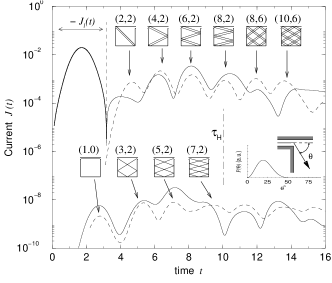
Figure 2: Quantum mechanical reflected and transmitted current through a square billiard (upper and lower solid curves respectively). Dashed lines indicate corresponding classical currents. The wave packet enters the billiard in the second mode $\alpha=2$; $\langle k\rangle=2.5w/\pi$. The insets show classical reflected and transmitted trajectories; the numbers in the parenthesis are the so-called winding numbers indicating how many times an electron traverses the billiard in the longitudinal and transverse directions. The inset to the right show an angular distribution of injected electrons $P(\theta)$ calculated in the Fraunhofer approximation for $\alpha=2$. The Heisenberg time $\tau_{H}$ is indicated by a dot-dashed line. The curves are shifted for clarity.

Let us first concentrate on the initial phase of the wave packet dynamics. Figure 2 shows the quantum-mechanical current for the square billiard in the time interval $t\lesssim 15$ (here and hereafter we measure time in units of the traversal time $t_{tr}=L/\langle v\rangle$, $\langle v\rangle=L/(\hbar\langle k\rangle/m^{*})$; the current is measured in units of $\hbar/2m^{*}a$). Our choice of the parameter of the wave packet $\sigma$ and $\langle k\rangle$ ensures that the spreading of the wave packet becomes noticeable only after relatively long time $t\gtrsim 50$. The initial period of time $0<t\lesssim 3$, when the current through the left lead $J_{l}(t)$ is negative, corresponds to a buildup phase when the wave packet enters the billiard. Having entered the billiard, the wave packet starts to leak out through the leads and the calculated QM currents $J_{l},J_{r}$ show a series of pronounced peaks. To outline the origin of these peaks we calculate the leakage current of a corresponding classical wave packet in the same billiard. In the classical calculations we take into account the diffractive effects in the leads in the framework of the standard Fraunhofer diffraction approximation by injecting the electrons with the corresponding angular distribution $P(\theta)$ (inset in Fig. 2 shows a calculated angular probability distribution for the lead geometry under consideration). A very good correspondence between the QM and the classical results allows us to ascribe each peak in the quantum-mechanical transmitted/reflected currents to a specific classical trajectory connecting the billiard leads, see inset in Fig. 2.

Figure 3: Quantum mechanical transmitted current through a square billiard for different incoming modes of the wave packet $\alpha=1,2,3$ with $\langle k\rangle\pi/w=1.5,2.5,3.5$ respectively. The upper curve indicates corresponding classical current. Vertical dotted lines are guides for an eye indicating the same positions of the peaks in the current. Dashed lines give the asymptotic power-law decay obtained by the best fit in the interval $80<t<2000$. The Heisenberg time $\tau_{H}$ is indicated by a dot-dashed line. The curves are shifted for clarity.

A relative height of each peak depends on the density of the corresponding trajectories, and the angular distribution for a given incoming mode $\alpha$. The effect of the later is clearly seen in Fig. 3, where the QM current in a square billiard was shown for three different incoming modes of the wave packet $\alpha=1,2,3$. At the initial stage of the current decay, $t\lesssim 20$, the positions of peaks are the same for all incoming modes, whereas their absolute values are different. This is explained by the fact that the angular distribution $P(\theta)$ is different for different $\alpha$, with its maximum being shifted to larger $\theta$ for higher modes $\alpha$. We conclude this discussion by noticing that all quantum billiards studied here exhibit similar characteristic peaks in the current at $t<\tau_{H}$ that can be explained in terms of corresponding classical trajectories.

Figure 4: Quantum mechanical reflected and transmitted current through a stadium-shaped billiard. Lower curves show corresponding classical currents. The wave packet enters the billiard in the second mode $\alpha=2$; $\langle k\rangle=2.5w/\pi$. The inset show a long-time assymptotics of classical escape along with the example of a bouncing-ball trajectory. Dashed lines give the asymptotic power-law decay obtained by the best fit in the interval $50<t<2000$. The Heisenberg time $\tau_{H}$ is indicated by a dot-dashed line. Time is measured in the units of the traversal time of the equivalent square of the same area. The curves are shifted for clarity.

Let us now focus on a long-time asymptotics of the wave packet dynamics. We start with a square billiard, see Fig. 3. Its classical escape rate is independent of the number of modes in the leads and is well approximated by a power law $\sim t^{-3}$. On the contrary, the calculated quantum-mechanical decay, does depend on the number of modes in the leads and follows the power law decay with the exponents $\xi=2.3,3,3.5$ for modes $\alpha=1,2,3$ correspondingly. These values are somehow different from those expected from Eq. (1), $\xi=2,3,4$. (In a billiard with two leads a number of decay channels is given by $M=2\alpha$).

One of the reasons for the above discrepancy may be related to the fact that in a billiard system the details of the coupling between the leads can be important for the selection of particular states that mediate transport through the system eigen (on the contrary, Eq. (1) corresponds to the case when all resonant states are excited with the same probability at $t=0$ ). Note that eq. (1) corresponds to the weak (tunneling) coupling between the leads and the dots in contrast to the regime of the open dot considered here. It is also worth to mention that Eq. (1) is based on the random matrix theory and similar stochastic approaches Lewenkopf ; Muller ; Fyodorov . The predictions of these theories tend to be rather general in nature and they usually fail to account for specific features of the geometry under consideration (such as details of the lead position, existence of periodic orbits, etc.).

Let us now discuss wave-packet evolution in a stadium-shaped billiard. Classically, this billiard exhibits chaotic dynamics, and its classical escape rate shows fast exponential decay, see Fig. 4. The quantum mechanical decay of such a system is however, qualitatively different. It obeys a power law similar to the one observed for the square. The difference between the classical and QM decay asymptotics becomes clearly discernible at the time scale corresponding to $\sim 50-100$ classical bounces in a billiard. With this respect it is important to stress that the difference in the power-law and the exponential escape for classical regular and chaotic systems becomes discernible at a comparable time intervalTB2 . Note that the billiard at hand is designed in such a way that the classical escape through the left lead changes its asymptotics from the exponential one to a slower power-law decay at $t\sim 500$. This behavior is caused by the bouncing-ball orbits Alt2 which are accessible via the left lead only (see inset in Fig. 4). It is interesting to note that the corresponding QM current through the left lead also starts to show slower decay at $t\sim 500$ in comparison to the right lead. We therefore speculate that, even though the long-time asymptotics of the QM and classical decays are qualitatively different, the QM decay still reflects some features of the underlying classical dynamics.

The qualitative difference between the QM and classical escape represents one of the main findings of the present work. We also find that the asymptotic decay of a quantum system obeys a power law that depends on the number of decay channels only, and is not sensitive to the nature of classical dynamics (chaotic or regular). This makes us conclude that quantum mechanics smears out the difference between classical chaotic and regular motion. With this respect it is important to stress that the difference in the classical decay rate in chaotic, regular or mixed system is often used in various semiclassical approaches to describe observed transport properties of the quantum systems (statistics of the fluctuations, the shape of weak localization, fractal conductance fluctuations, etc.) Marcus_Andy ; Smilansky ; Jalabert ; Baranger ; Ker . We demonstrate however, that the crossover to the QM power law decay may occur at the same time scale when the difference between classical regular and chaotic systems becomes discernible. Our findings thus strongly indicate that some of the SC predictions should be used with certain caution or even be revised. Finally, the results reported in the present paper can be tested experimentally in the variety of systems including semiconductor quantum dots Marcus_Andy , microwave cavities Stoeckmann , acoustical acoustics and optical billiards optics .

- (1) C. Marcus et al., Phys. Rev. Lett. 69, 506 (1992); A. S. Sachrajda et al., ibid., 80, 1948 (1998).
- (2) S. Tomsovic and E. J. Heller, Phys. Rev. Lett. 67, 664 (1991).
- (3) Y. V. Fyodorov and H.-J. Sommers, J. Math. Phys. 38 1918 (1997).
- (4) P. W. Brouwer, K. M. Frahm, and C. W. J. Beenakker, Phys. Rev. Lett. 78, 4737 (1997).
- (5) W. Bauer and G. F. Bertsch, Phys. Rev. Lett. 65, 2213 (1990).
- (6) R. Blümel, and U. Smilansky, Phys. Rev. Lett. 60, 477 (1988).
- (7) R. A. Jalabert, H. U. Baranger, and A. D. Stone, Phys. Rev. Lett. 65, 2442 (1990).
- (8) R. Kerzmerik, Phys. Rev. B 54, 10 841 (1996).
- (9) H. U. Baranger, R. A. Jalabert, and A. D. Stone, Phys. Rev. Lett. 70, 3876 (1993).
- (10) C. H. Lewenkopf and H. A. Weidenmüller, Ann. Phys. 212, 53 (1991).
- (11) F.-M. Dittes, H. L Harney, and A. Müller, Phys. Rev. A 45, 701 (1992); H. L Harney, F.-M. Dittes, and A. Müller, Ann. Phys. 220, 159 (1992).
- (12) H. Alt et al., Phys. Rev. Lett. 74, 62 (1995).
- (13) T. Blomquist and I. V. Zozoulenko, Phys. Rev. B 64, 195301 (2001).
- (14) T. Palm, J. Appl. Phys. 74, 3551 (1993); J. B. Wang and S. Midgley, Phys. Rev. B 60 13668 (1999).
- (15) J. A. Støvneng and E. H. Hauge, Phys. Rev. B 44 13586 (1991).
- (16) I. V. Zozoulenko, F. A. Maaø and E. H. Hauge, Phys. Rev. B . 53, 7975 (1996); ibid., 7987 (1996).
- (17) I. V. Zozoulenko et al., Phys. Rev. B 55, R10209 (1997); I. V. Zozoulenko and K.-F. Berggren, Phys. Rev. B 56, 6931 (1997).
- (18) H. Alt et al., Phys. Rev. E 53, 2217 (1996).
- (19) J. Stein, H.-J. Stöckmann, and U. Stoffregen, Phys. Rev. Lett. 75, 53 (1995).
- (20) J. de Rosny, A. Tourin, and M. Fink, Phys. Rev. Lett. 84, 1693 (2000).
- (21) N. Friedman et al., Phys. Rev. Lett. 86, 1518 (2001); V. Milner et al. ibid., 1514 (2001).