Stretching of a polymer below the $\Theta$ point

Abstract

The unfolding of a polymer below the $\theta$ point when pulled by an external force is studied both in $d=2$ on the lattice and in $d=3$ off lattice. A ground state analysis of finite length chains shows that the globule unfolds via multiple steps, corresponding to transitions between different minima, in both cases. In the infinite length limit, these intermediate minima have a qualitative effect only in $d=2$. The phase diagram in $d=2$ is determined using transfer matrix techniques. Energy-entropy and renormalization group arguments are given which predict a qualitatively correct phase diagram and a change of the order of the transition from $d=2$ to $d=3$.

The recent refinements in experimental techniques employing optical tweezers[1], atomic force microscopes[2], soft microneedles[3], make potentially possible for researchers to monitor the behaviour under tension and stress of various biopolymers and then to elucidate the mechanism of some force-driven phase transitions occurring at the single molecule level, such as the unfolding of the giant titine protein[4], the stretching of single collapsed DNA molecules[5, 6], the unzipping of RNA and DNA[1]. Theoretically, on the other hand, quite a few statistical mechanics models have been subsequently proposed in order to explain these experimental results and to identify the physical mechanisms behind these phase transitions[7, 8, 9, 10, 11, 12, 13, 14, 15]. In this work we focus on two theoretical models aimed at understanding the unfolding behaviour of polymers in a poor[16] solvent (globules), i.e. below the theta temperature, $T_{\theta}$.

This is motivated by the vast number of experimental results in the literature. In particular, various force vs elongation ($f$ vs $x$) curves have been recorded in experiments studying these phenomena[5, 6]. In most cases a curve consisting of three distinct regimes, and in particular displaying a plateau for intermediate stretch[5, 6], have been observed; whereas in a few examples, for shorter polymers, a stick-release pattern with histeresis has been found. The first observation is in good agreement with the mean field theory proposed in Ref.[7], and the plateau strongly suggests the presence of a first order phase transition (see also the recent measurements in [6]). Our results suggest that there might be more than one possible shape for the $f$ vs. $x$ curves according to $d$, the spatial dimension and to polymer length, so that a different behaviour occurs when mean field theory[17] is qualitatively incorrect. These models have a remarkable interest even on a purely theoretical ground. First, the numerical study recently performed in [11] has suggested the possibility that the transition is second order in $d=2$ and first order in $d=3$. This has been confirmed to some extent in a study of the model on a hierarchical lattice with fractal dimension two[12]. The $d=2$ case is important as it is below the upper critical dimension for theta collapse and mean field predictions may well be incorrect. A thourough analysis and a clear physical mechanism underlying the difference of the nature of the transition as $d$ changes are then needed. Second, the mean field analysis of Ref.[10] has suggested there could be a re-entrant region in the phase diagram for low temperature similar to what happens for DNA unzipping[15]. However the exact results in[12] prove mean field is not valid in $d=2$.

Then, our aim here is to describe theoretically the unfolding transition of globules not relying on the mean field approximation. We first characterize the evolution of the ground states of a finite polymer as the pulling force increases. This will help to understand the thermodynamics. In particular, we compute the phase diagram in the temperature–force $(T,f)$-plane in $d=2$ on the lattice, where we can use the transfer matrix method (Fig. 2) together with exact enumerations (Fig. 1).

We begin by considering a self-avoiding walk (SAW) on the square lattice with fixed origin. The model partition function (generating function) in the canonical ensemble in which $T$ and $f$, the stretching force, are fixed is:

$$Z_{N}(f,T)=\sum_{\mathcal{C}}e^{-\beta H(\mathcal{C})}=\sum_{b,\mathbf{R}}w_{o\mathbf{R}}(N,b)e^{\beta(b\epsilon+fR_{x})}$$ (1)

where $N$ is the number of monomers (including the origin) of the SAW, $H(\mathcal{C})$ (referred to a configuration $\mathcal{C}$, i.e. to a SAW) is the energy of a SAW, $b$ is the number of pairs of neighboring occupied sites not adiacent along the chain, $\beta\equiv\frac{1}{T}$ is the inverse temperature, $w_{o\mathbf{R}}(N,b)$ is the number of configurations of a SAW with fixed origin $o$ and end-to-end distance $\mathbf{R}$, of lenght $N$ and $b$ contacts, $R_{x}$ is the projection along the force direction ($x$ axis) of $\mathbf{R}$. We take both the Boltzmann constant and $\epsilon$ equal to one.

When $T$ is low, one may look for the ground states among the rectangles of sides $L_{x}$ and $L_{y}$ that are completely covered by the SAW (in other words such that $L_{x}L_{y}=N$, where we neglect the small effects arising when this rectangle cannot be constructed with both $L_{x,y}$ integers). The energy of this rectangular hamiltonian walk with a non zero $f$ is $-H(N\equiv L_{x}L_{y},L_{x})=N-L_{x}-\frac{N}{L_{x}}+1+f(L_{x}-1)$. The minimum of $H(N,L_{x})$ for given $N$ with respect to $L_{x}$ yields the most stable configuration for various values of $f$. The minimum occurs for an $f$-dependent value of $L_{x}^{0}\equiv L_{x}^{0}(N,f)$, namely $L_{x}^{0}(N,f)=\sqrt{\frac{N}{1-f}}$. For any $f<1$ one has a compact configuration. However, when the critical value $f=1$ (for $T=0$) is reached all integer values of $L_{x}$ from $N$ (stretched coil) to $L_{x}\sim N^{1/2}$ (compact globule) become degenerate for large $N$. Note that this does not hold in $d=3$ where it is well known that there is a Rayleigh instability in the thermodynamic limit[6, 7, 11]. This can be seen by comparing the globule energy - which in $d=3$ is $2N$ in the large $N$ limit - with the energy of a parallelepiped, with elongation along $\vec{f}$ equal to $L_{x}$ and with edges $L_{y}=L_{z}$ in the perpendicular plane. The force above which (for $T=0$) the parallepiped is a better ground state than the three-dimensional globule is $2L_{y}$ ($L_{y}\ll N^{1/3}$), and there is no longer any degeneracy at the critical force $f_{c}=2$ (at $T=0$).

In Fig. 1a we sketch the situation in $d=2$. The minima hierarchy, shown in the shaded area in the top panel, affects the low $T$ region of the $<x>$ (average elongation) vs. $f$ curves for finite length (bottom panel). However, only one transition survives in the large $N$ limit and represents a true phase transition (as represented in Fig. 1a by the shaded wedge ending in just one point in the $N^{-1}=0$ axis). Similarly, when $T$ is raised the multi-step character of the $<x>$ vs. $f$ curves is lost due to fluctuations which blur the ground state dominance in the partition. In Fig. 1b we show the analogous picture for a $3d-$model discussed below. Short chains in $d=2$ and $3$ behave similarly whereas in the infinite length limit the $d=3$-case shows an abrupt unfolding transition.

We now turn to the thermodynamic behaviour of the SAW model on a square lattice. We use the transfer matrix (TM) technique, following Refs.[19, 20, 21].

Let us introduce briefly the principal features of the TM approach: the partition function of a polymer of $N$ sites is given by Eq. (1), with $f=0$. In the thermodynamic limit ($N\rightarrow\infty$) we expect that $Z_{N}(T)\sim[\mu(T)]^{N}$, then the free energy per monomer ${\mathcal{F}}$ is simply, ${\mathcal{F}}=-T\log\mu(T)$. It is more convenient[19] to introduce the following generating function ($z$ is the step fugacity)

$$g_{o\mathbf{R}}=\sum_{N,b}z^{N}e^{\beta b}w_{o\mathbf{R}}(N,b)$$ (2)

It is known that for $z<z^{c}(T)=1/\mu(T)$, the inverse SAW connectivity, $g_{o\mathbf{R}}\sim\exp(-R_{x}/\xi(z,T))$, where $\xi(z,T)$ is the correlation length and $R_{x}$ is the projection of ${\mathbf{R}}$ along $x$. We study the stretching of an interacting SAW in a strip of finite size $L$ along $y$ and infinite length along $x$. It is possible to define[19] an $L$-dependent correlation length $\xi_{L}(z,T)$ via the formula $\xi_{L}(z,T)=-\frac{1}{\log\lambda_{L}(z,T)}$, where $\lambda_{L}(z,T)$ is the largest eigenvalue of the transfer matrix, that equals $1$ at $z=z^{c}_{L}(T)$. We apply the phenomenological renormalization, to find successive estimates for $z_{c}(T)=\lim_{L\rightarrow\infty}z_{L}^{c}(T)$. Including the force via Eq. (1), the equation for the critical force $f_{c}(T)$ is then ideally found via:

$$f_{c}=-T\lim_{z\to z_{c}(T)^{-}}\lim_{L\to\infty}\log{\lambda_{L}}.$$ (3)

The order of the limits in Eq. (3) and a correct choice of the boundary conditions (see below) are crucial [22].

In Fig. 2 the phase diagram for the stretched interacting SAW is shown. With the TM, a right choice of the boundary conditions is needed[19, 20, 21]. We have used both periodic (PBC) and free boundary conditions (FBC). PBC have been employed to get the best estimate of $z_{c}(T)$ through phenomenological renormalization. This value is then used with FBC, to find the correct $L$-dependent critical eigenvalue $\lambda_{L}(z_{c}(T),T)$. Finally, adopting the extrapolation algorithm of [23], $\lim_{L\rightarrow\infty}\lambda_{L}(z_{c}(T),T)$ is obtained which, through Eq. (3), allows to get the phase diagram. As expected, in the case of FBC, there are oscillations in data going from odd $L$ to even $L$. As usual in this context, a separated analysis of even and odd $L$ data was necessary for obtaining a better convergence (see Fig. 2). One point on the transition line obtained previously in [11], is recovered here.

One can get an approximate description of the transition if one requires that the globule and coil phases coexist. The globule free energy is easily estimated in terms of hamiltonian walks[16]. On a square lattice the energy is simply given by minus the length of the polymer whereas the entropy is given in terms of the number of hamiltonian walks which grows exponentially with $N$[16]. Thus the globule free energy per monomer is ${\mathcal{F}}_{g}=-1-T\log(4/e)$ where we have used the accurate mean field estimate of the entropy as given in [24]. The coil free energy ${\mathcal{F}}_{c}$ is approximated as that of an unconstrained random walk in presence of a pulling force and contacts are neclected. We thus get ${\mathcal{F}}_{c}=-\log(2(1+\cosh(\beta f)))$. At coexistence one finds $f_{c}(T)=T{\cosh}^{-1}(2\exp(1/T-1)-1)$ (the continuos curve in Fig. 2).

We note that $f_{c}(0)=1$ is the exact result and at low $T$ the phase diagram displays a reentrant region. As $T\to T_{\theta}$, $f$ approaches $0$ rather smoothly, consistently with the prediction $f\sim(T_{\theta}-T)^{\frac{\nu_{\theta}}{\phi_{\theta}}=\frac{4}{3}}$ [12]. Within the TM approach one can also infer the order of the transition. To do this we observe that, if for $z\to z_{c}(T)^{-}$:

$$\lambda(z_{c}(T),T)-\lambda(z,T)\sim(z_{c}(T)-z)^{\Delta},$$ (4)

then $\Delta<1$ ($\Delta=1$) means a second (first) order transition, as $<x>\sim(f-f_{c})^{\frac{1}{\Delta}-1}$ for $f\sim f_{c}$. Our data at not too low $T$ are compatible with a second order transition (inset of Fig. 2).

Inspired by exact renormalization group (RG) on the Sierpinski lattices [12], and on approximate RG in $d-$ dimensional lattices [25], we propose the following simplified real space RG which rationalizes our results. The RG recursions relations can be written for the generating function representing polymers traversing a hypercube of linear size $1$ once, $A$, and $2^{d-1}$-times, $B$ (Fig. 3). The terms $A$ and $B$ represent parts of the chain which are in the coil and globular state respectively. The recursion relations can be calculated as in Ref.[18] or by enumerating the SAWs on $2\times 2$ or $2\times 2\times 2$ cells as in [25]. To leading order in $A$ at $0\neq T\ll T_{\theta}$

$$A^{\prime}=A^{2}+\alpha(d)A^{2}B^{2},\quad B^{\prime}=\gamma(d)B^{2^{d}},$$ (5)

where $\alpha(d)$ and $\gamma(d)$ are $d-$dependent constants. There are three fixed points in the flux in Eq. 5: $A=0$, $B=B^{*}=\gamma(d)^{-\frac{1}{2^{d}-1}}$ corresponds to the globular phase, $(A,B)=(1,0)$ to the coil phase, while the last non-trivial fixed point $A=A^{*}=\frac{1}{1+\alpha(d)(B^{*})^{2}}$, $B=B^{*}$ characterizes the unfolding transition. The value of the term $\alpha(d)$ affects the behaviour of the RSRG flux near the fixed point $(A^{*},B^{*})$. One can see[26] that $\alpha(d)\neq 0$ if $d=2$ and is $0$ in $d>2$. When $\alpha(d)\neq 0$ (i.e. in $d=2$), the RG flux is smooth near $(A^{*},B^{*})$ and the critical fugacity near $f=f_{c}(T)$ behaves as $z_{c}(f_{c}(T),T)-z_{c}(f,T)\sim(f-f_{c}(T))^{2}$ signalling a second order transition with $\Delta=1/2$ in Eq.4. On the other hand when $\alpha(d)=0$ (i.e. $d>2$), the transition is first order and two-state like. The presence of the mixed term in Eq. (5) is crucial and enhances the entropy of the coil phase since it contributes to $A^{\prime}$. Consequently, the $d=2$ two-state approximation in Fig. 2 gives a transition line which is higher than the numerical result for $0\neq T\ll T_{\theta}$. The entropy gain in the stretched coil, as $T\to 0$, is hampered as it costs a finite surface energy (dominant as $T\to 0$) to change locally an elongated globular region into a coil and vice-versa. This is why the solid curve in Fig. 2 matches our numerics as $T\to 0$.

Let us now discuss the $d=3$ case. The model we used is the freely jointed chain (FJC) (see e.g. [16]) in the continuum (off lattice). The FJC is subject to a compacting pairwise attractive potential between non-consecutive beads and to a stretching force $\vec{f}$ at the extrema. The pairwise potential is chosen to be an asymmetric square well with a hard core radius, $2R_{hc}$, which acts between non-consecutive beads along the chain, and an attraction range $R_{1}>2R_{hc}$, i.e. the distance up to which the particles interact. We have checked that the results reported in the following do not appreciably depend on the two-body potential details. The parameters we have used to generate the configurations shown in Fig. 1b (top panel) are $R_{hc}=0.6$, $R_{1}=1.6$ where the unit length is the distance between sucessive beads along the chain.

The ground states of short chains (up to $N=30$ bead long) has been determined by performing simulated annealing employing Monte-Carlo dynamical simulations. The FJC is evolved dynamically by means of three sets of moves: the pivot, reptation and crankshaft moves[27]. We lower $T$ during the simulation according to a standard annealing schedule. We found evidence also in this $d=3$ case that the unfolding of a finite length homopolymer proceeds in a multistep fashion. The collapsed globule first orients itself along the pulling force as soon as there is a nonzero $f$. At larger $f$ the globule is slightly elongated (much less than in the $d=2$ case) and after this a helix forms followed by a zig-zag curve and finally by a stretched coil. This succession of minima, shown in fig. 1b is intriguing for a two-fold reason: firstly because it suggests that helices, one of the well known building block of proteins, come out rather naturally as one of a few stable minima of a homopolymer in a poor solvent subject to a finite stretching force; secondly because the unfolding transition of a finite polymer in this model appears to be markedly different from a globule-to-coil (two-state) transition. The mean field picture of an all or none transition is recovered for infinite length. The situation is depicted in Fig. 1b. Since in $d=3$ the transition is first order, the mean field treatment is correct in the thermodynamic limit. The fact that helices become better ground states than compact globules could be easily verifiable in experiments done in the fixed force ensemble. These can now be confidently performed, with not more substantial difficulties than the more conventional ones, performed in the fixed stretch ensemble. Indeed the stick-release pattern reported in Ref.[5] shows several different peaks in the $f$ vs. $<x>$ curve, and is compatible with a ‘multi-step transition’ in which the globule undergoes more than one conformational changes (signalled by the peaks) during the unfolding. Intriguingly, this pattern is reported for smaller polymers, a fact which would be in agreements with our findings; whereas for large $N$ this effect is much less important and the curves have a single (dominant) plateau.

Helices appear as ground states for a potential consisting of a force term and a hydrophobic contact potential because they are both elongated and offer a good shielding from the outside solvent to the monomers lying in its interior. Note also that helices arise as optimal states of tubes of non-zero thickness subject to compaction[28]. If a worm-like chain is used instead of the FJC, the picture should not change, because the elongated states such as the helices and the zig-zag are stiffer than the collapsed globule (sharp corners between successive monomers are necessary in this state) and so should be even more favoured as $f$ is increased.

In conclusion, we have discussed the unfolding transition of a homopolymer under the action of an external pulling force in $d=2$ on the lattice and in $d=3$ off lattice. A ground state analysis shows that for finite length polymers, the unfolding is not abrupt, rather it occurs via a multi step sequence of states. These are more elongated than the globule and make more contacts than a coil. In $d=3$ helices arise naturally as ground states at intermediate forces. For infinite polymers, on the other hand, the situation is different: in $d=3$ the intermediate ground states disappear due to the Rayleigh instability, and the transition is effectively two-state, whereas in $d=2$ they survive in the thermodynamic limit. Indeed, from the transfer matrix results, it is apparent that the mean field hypothesis is incorrect in $d=2$ even at rather low $T$: the transition is second order as also found in Ref. [11] although the prediction of the re-entrant region agrees with the TM results. Furthermore a renormalization group based argument is in agreement with this picture.

This work was supported by Cofin 2001 and FISR.

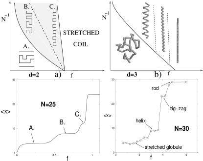
FIG. 1.: a) $d=2$ Schematic diagram of minima for polymers of different sizes (top) and low $T$ $<x>$ vs. $f$ curve for $N=25$ (bottom) found with exact enumerations in $d=2$. b) d=3: Same as in a), except that the $<x>$ vs. $f$ curve (bottom) is for $N=30$ and is found by simulated annealing.

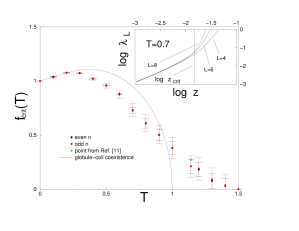
FIG. 2.: Phase diagram for the stretching of a SAW on a $2d$-lattice, obtained with the TM technique. Inset: plot of $\log{\lambda}$ vs. $\log{z}$ for $T=0.7$.

FIG. 3.: Representation of the generating functions $A$ and $B$ in the text (for $d=3$) at a generic level of iteration in the RG. Thick lines represent portions of the SAW that enter through a vertex and go out from another one.

REFERENCES

- [1] U. Bockelmann, P. Thomen, B. Essevaz-Roulet, V. Viasnoff, F. Heslot, Biophys. J. 82, 1537 (2002).
- [2] M. Reif, H. Clausen-Schaumann, H. E. Gaub, Nature Struc. Biol. 6, 346 (1999).
- [3] A. Kishino, T. Yanagida, Nature 34, 74 (1988).
- [4] M. Rief et al., Science 276, 1109 (1997), M. S. Z. Kellermayer et al., Adv. Exp. Med. Biol. 481, 111 (2000).
- [5] C. G. Baumann et al., Biophys. J. 78, 1965 (2000).
- [6] B. J. Haupt, T. J. Senden, E. M. Sevick, Langmuir 18, 2174 (2002).
- [7] A. Halperin, E. B. Zhulina, Europhys. Lett. 15, 417 (1991).
- [8] D. K. Klimov, D. Thirumalai, Proc. Natl. Acad. Sci. USA 96, 6166 (1999).
- [9] T. A. Vilgis, A. Johner, J. F. Joanny, Eur. Phys. J. E 2, 289 (2000).
- [10] P. L. Geissler, E. I. Shakhnovich, Phys. Rev. E 65 056110 (2002); cond-mat/0111317.
- [11] P. Grassberger, H. Hsu, Phys. Rev. E 65, 031807 (2002).
- [12] D. Marenduzzo, A. Maritan, F. Seno, J. Phys. A 35, L233 (2002).
- [13] M. Cieplak, T. X. Hoang, M. O. Robbins, cond-mat/0112200, cond-mat/0112201.
- [14] S. M. Bhattacharjee, J. Phys. A 33, L423 (2000); D. K. Lubensky, D. R. Nelson Phys. Rev. Lett. 85 1572 (2000); S. Cocco, R. Monasson, J. F. Marko, Proc. Natl. Acad. Sci. USA 98, 8608 (2001), E. Carlon, E. Orlandini, A. L. Stella Phys. Rev. Lett. 88, 198101 (2002).
- [15] D. Marenduzzo, S. M. Bhattacharjee, A. Maritan, E. Orlandini, F. Seno, Phys. Rev. Lett. 88, 028102 (2002).
- [16] C. Vanderzande, Lattice models of polymers, Cambridge University Press (1998).
- [17] Note that we use ‘mean field theory’ in a broader sense, including approaches which consider the relative stability of the globule and the coil only (see also [10]). Mean field theories should be all equivalent as regards universality.
- [18] D. Dhar, J. Vannimenus, J. Phys. A 20, 199 (1987).
- [19] B. Derrida, J. Phys. A 14, L5 (1981).
- [20] A. Trovato, F. Seno, Phys. Rev. E 56, 131 (1997).
- [21] H. Saleur, J. Stat. Phys. 45, 419 (1986).
- [22] This and other subtleties of the TM approach (unnecessary here) will be addressed in detail elsewhere.
- [23] M. Henkel, G. Schutz, J. Phys. A 21, 2617 (1988)
- [24] S. Lise, A. Maritan and A. Pelizzola, Phys. Rev. E 58, R5241 (1998).
- [25] A. Maritan, F. Seno, A. L. Stella, Physica A 156, 679 (1989).
- [26] These facts can be proved exactly in a family of Sierpinski gaskets (see [12] for an example), where is the fractal dimension. On conventional lattices, an approximate RG treatment as in [25] gives qualitatively the same behaviour. Details will be given in a future work.
- [27] A. D. Sokal, Nucl. Phys. B, Suppl. 47, 172 (1996)
- [28] A. Maritan, C. Micheletti, A. Trovato, J. R. Banavar, Nature 406, 287 (2000).