Statistical stability in time reversal

Abstract

When a signal is emitted from a source, recorded by an array of transducers, time reversed and re-emitted into the medium, it will refocus approximately on the source location. We analyze the refocusing resolution in a high frequency, remote sensing regime, and show that, because of multiple scattering, in an inhomogeneous or random medium it can improve beyond the diffraction limit. We also show that the back-propagated signal from a spatially localized narrow-band source is self-averaging, or statistically stable, and relate this to the self-averaging properties of functionals of the Wigner distribution in phase space. Time reversal from spatially distributed sources is self-averaging only for broad-band signals. The array of transducers operates in a remote-sensing regime so we analyze time reversal with the parabolic or paraxial wave equation.

1 Introduction

In time reversal experiments a signal emitted by a localized source is recorded by an array and then re-emitted into the medium time-reversed, that is, the tail of the recorded signal is sent back first. In the absence of absorption the re-emitted signal propagates back toward the source and focuses approximately on it. This phenomenon has numerous applications in medicine, underwater acoustics and elsewhere and has been extensively studied in the literature, both from the experimental and theoretical points of view [12, 13, 14, 15, 16, 20, 24, 25, 31]. Recently time reversal has been also the subject of active mathematical research in the context of wave propagation and imaging in random media [2, 3, 4, 7, 8, 9, 32]. A schematic description of a time reversal experiment is presented in Figure 1.

(-0.04*0.55) $\frac{\lambda L}{a_{e}}$

(0.45*0.05) $L$

(1.03*0.65) $a$

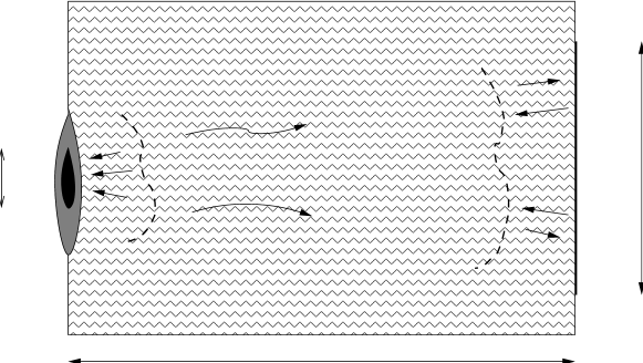
Fig. 1: A pulse propagates toward a time reversal array of size $a$. The propagation distance $L$ is large compared to $a$. The ambient medium has a randomly varying index of refraction with a typical correlation length that is small compared to $a$. The signal is time reversed at the array and sent back into the medium. The back propagated signal refocuses with spot size $\lambda L/a_{e}$, where $a_{e}$ is the effective aperture of the array (Section 3.3).

For a point source in a homogeneous medium, the size of the refocused spot is approximately $\lambda L/a$, where $\lambda$ is the central wavelength of the emitted signal, $L$ is the distance between the source and the transducer array and $a$ is the size of the array. We assume here that the array is operating in the remote-sensing regime $a\ll L$. Multiple scattering in a randomly inhomogeneous medium creates multipathing, which means that the transducer array can capture waves that were initially moving away from it but get scattered onto it by the inhomogeneities. As a result, the array captures a wider aperture of rays emanating from the original source and appears to be larger than its physical size. Therefore, somewhat contrary to intuition, the inhomogeneities of the medium do not destroy the refocusing but enhance its resolution. The refocused spot is now $\lambda L/a_{e}$, where $a_{e}>a$ is the effective size of the array in the randomly scattering medium, and depends on $L$. The enhancement of refocusing resolution by multipathing is called super-resolution [7]. The time reversed pulse is also self averaging and refocusing near the source is therefore statistically stable, which means that it does not depend on the particular realization of the random medium. There is some loss of energy in the refocused signal because of scattering away from the array but this can be overcome by amplification, up to a point.

The purpose of this paper is to explore in detail the mathematical basis of pulse stabilization, beyond what was done in [7]. We want to explore in particular in what regime of parameters statistical stability is observed in time reversal. We show here that for high frequency waves in a remote sensing regime, spatially localized sources lead to statistically stable super-resolution in time reversal, even for narrow-band signals. We also show that when the source is spatially distributed, only for broad-band signals do we have statistical stability in time reversal. The regime where our analysis holds is a high frequency one, more appropriate to optical or infrared time reversal than to ultrasound, sonar or microwave radar. In this regime we can make precise what spatially localized or distributed means (see Section 3.1). The numerical simulations in [7] and [8], which are set in ultrasound or underwater sound regime, indicate that time reversal is not statistically stable for narrow-band signals even for localized sources. Only for broad-band signals is time reversal statistically stable in the regime of ultrasound experiments or sonar.

If the aperture of the transducer array is small $a/L\ll 1$, the Fresnel number ${L}/(ka^{2})$ is of order one, and the random inhomogeneities are weak, which is often the case, we may analyze wave propagation in the paraxial or parabolic approximation [29]. The wave field is then given approximately by

$$u(t,{\bf x},z)=\frac{1}{2\pi}\int e^{i\omega(z/c_{0}-t)}\psi(z,{\bf x};\omega/c_{0})d\omega$$ (1)

where the complex amplitude $\psi$ satisfies the parabolic or Schrödinger equation

$$2ik\psi_{z}+\Delta_{\bf x}\psi+k^{2}(n^{2}-1)\psi=0.$$ (2)

Here ${\bf x}=(x,y)$ are the coordinates transverse to the direction of propagation $z$, the wave number $k=\omega/c_{0}$ and $n({\bf x},z)=c_{0}/c({\bf x},z)$ is the random index of refraction relative to a reference speed $c_{0}$. The fluctuations of the refraction index

$$\sigma\mu(\frac{{\bf x}}{l},\frac{z}{l})=n^{2}({\bf x},z)-1$$ (3)

are assumed to be a stationary random field with mean zero, variance $\sigma^{2}$, correlation length $l$ and normalized covariance with dimensionless arguments

$$R({{\bf x}},{z})=E\{\mu({{\bf x}}+{{\bf x}}^{\prime},{z}+{z}^{\prime})\mu({{\bf x}}^{\prime},{z}^{\prime})\}.$$ (4)

A convenient tool for the analysis of wave propagation in a random medium is the Wigner distribution [19, 28] defined by

$$W(z,{\bf x},{\bf p})=\frac{1}{(2\pi)^{d}}\int_{{\mathbb{R}}^{d}}e^{i{\bf p}\cdot{\bf y}}\psi({\bf x}-\frac{{\bf y}}{2},z)\overline{\psi({\bf x}+\frac{{\bf y}}{2},z)}d{\bf y}$$ (5)

where $d=1$ or $2$ is the transverse dimension and the bar denotes complex conjugate. The Wigner distribution may be interpreted as phase space wave energy and is particularly well suited for high frequency asymptotics and random media [28]. The quantity of principal interest in time reversal, the time-reversed and back-propagated wave field, can be also expressed in terms of the Wigner distribution (see Section 3.1). The self-averaging properties of the back-propagated field are related to the self-averaging properties of functionals of the Wigner distribution in the form of integrals of $W$ over the wave numbers ${\bf p}$.

In the next Section we introduce a precise scaling that corresponds to (a) high frequency, (b) long propagation distance, (c) narrow beam propagation, and (d) weak random fluctuations. In the asymptotic limit where the small parameters go to zero the Wigner distribution satisfies a stochastic partial differential equation (SPDE), a Liouville-Ito equation, that has the form

$$dW(z,{\bf x},{\bf p};k)=\left(-\frac{{\bf p}}{k}\cdot\nabla_{{\bf x}}W+\frac{k^{2}D}{2}\Delta_{{\bf p}}W\right)dz-\frac{k}{2}\nabla_{{\bf p}}W\cdot d{\bf B}({\bf x},z)$$ (6)

where ${\bf B}({\bf x},z)$ is a vector-valued Brownian field with covariance

$$E\{B_{i}({\bf x}_{1},z_{1})B_{j}({\bf x}_{2},z_{2})\}=-\left(\frac{\partial^{2}R_{0}(({\bf x}_{1}-{\bf x}_{2}))}{\partial x_{i}\partial x_{j}}\right)z_{1}\wedge z_{2},$$ (7)

where $z_{1}\wedge z_{2}=\min\{z_{1},z_{2}\}$, and in the isotropic case

$$D=-\frac{R_{0}^{{}^{\prime\prime}}(0)}{4},~{}~{}~{}R_{0}({\bf x})=\int_{-\infty}^{\infty}R({\bf x},s)ds.$$ (8)

In Section 2.5 we analyze this SPDE in the asymptotic limit of small correlation length for ${\bf B}({\bf x},z)$ in the transverse variables ${\bf x}$, and show that $W(z,{\bf x},{\bf p};k)$’s with different wave vectors ${\bf p}$ are uncorrelated. From this decorrelation property we deduce that for localized sources the time-reversed, back-propagated field is self-averaging, even for narrow-band signals. For distributed sources it is self-averaging only for broad-band signals. We show in detail in Section 3 how the asymptotic theory is used in time reversal. In Appendix A we introduce other scalings which lead to the same averaged SPDE but we do not analyze them in detail.

Throughout the paper we define the Fourier transform by

$$\hat{f}({\bf k})=\int d{\bf x}e^{-i{\bf k}\cdot{\bf x}}f({\bf x})$$

so that

$$f({\bf x})=\int\frac{d{\bf k}}{(2\pi)^{d}}e^{i{\bf k}\cdot{\bf x}}\hat{f}({\bf k}).$$

G. Papanicolaou was supported in part by grants AFOSR F49620-01-1-0465, NSF DMS-9971972 and ONR N00014-02-1-0088, L. Ryzhik by NSF grant DMS-9971742, an Alfred P. Sloan Fellowship and ONR grant N00014-02-1-0089. K. Solna by NSF grant DMS-0093992 and ONR grant N00014-02-1-0090.

2 Scaling and asymptotics

2.1 The rescaled problem

To carry out the asymptotic analysis we begin by rewriting the Schrödinger equation (2) in dimensionless form. Let $L_{z}$ and $L_{\bf x}$ be characteristic length scales in the propagation direction, as, for example, the distance $L$ between the source and the transducer array for $L_{z}$ and the array size $a$ for $L_{x}$. We introduce a dimensionless wave number $k^{\prime}=k/k_{0}$ with $k_{0}=\omega_{0}/c_{0}$ and $\omega_{0}$ a central frequency. We rescale ${\bf x}$ and $z$ by ${\bf x}=L_{\bf x}{\bf x}^{\prime}$, $z=L_{z}z^{\prime}$ and rewrite (2) in the new coordinates dropping primes:

$${2i}k\displaystyle\frac{\partial{\psi}}{\partial{z}}+\frac{L_{z}}{k_{0}L_{\bf x}^{2}}\Delta\psi+k^{2}k_{0}L_{z}\sigma\mu\left(\frac{{\bf x}L_{\bf x}}{l},\frac{zL_{z}}{l}\right)\psi=0.$$ (9)

The physical parameters that characterize the propagation problem are: (a) the central wave number $k_{0}$, (b) the strength of the fluctuations $\sigma$, and (c) the correlation length $l$. We introduce now three dimensionless variables

$$\delta=\frac{l}{L_{\bf x}},~{}~{}\varepsilon=\frac{l}{L_{z}},~{}~{}\gamma=\frac{1}{k_{0}l}$$ (10)

which are the reciprocals of the transverse scale relative to correlation length, the reciprocal of the propagation distance relative to correlation length, and the central wave length relative to the correlation length. We will assume that the dimensionless parameters $\gamma$, $\sigma$, $\varepsilon$ and $\delta$ are small

$$\gamma~{}\ll~{}1;~{}~{}~{}\sigma~{}\ll~{}1;~{}~{}~{}\delta~{}\ll~{}1;~{}~{}~{}\varepsilon~{}\ll~{}1~{}.$$ (11)

This is a regime of parameters where super-resolution phenomena can be observed.

To make the scaling more precise we introduce the Fresnel number

$$\theta=\frac{L_{z}}{k_{0}L_{\bf x}^{2}}=\gamma\frac{\delta^{2}}{\varepsilon}.$$ (12)

We can then rewrite the Schrödinger equation (9) in the form

$$2ik\theta\psi_{z}+\theta^{2}\Delta_{\bf x}\psi+\frac{k^{2}\delta}{\varepsilon^{1/2}}\mu(\frac{{\bf x}}{\delta},\frac{z}{\varepsilon})\psi=0.$$ (13)

provided that we relate $\varepsilon$ to $\sigma$ and $\delta$ by

$$\varepsilon=\sigma^{2/3}\delta^{2/3}.$$ (14)

One way that the asymptotic regime (11) can be realized is with the ordering

$$\theta~{}\ll~{}\varepsilon~{}\ll~{}\delta~{}\ll 1~{},$$ (15)

and $\gamma~{}\ll~{}\sigma^{4/3}\delta^{-2/3}$, corresponding to the high-frequency limit. We see from the scaled Schrödinger equation (13) that this regime can be given the following interpretation. We have first a high frequency limit $\theta\to 0$, then a white noise limit $\varepsilon\to 0$, and then a broad beam limit $\delta\to 0$. We will analyze in detail and interpret these limits in the following Sections. Another scaling in which (11) is realized is $\varepsilon~{}\ll~{}\theta~{}\ll\delta~{}\ll 1$. This is a regime in which the white noise limit is carried out first, then the high frequency limit and then the broad beam limit. We do not analyze this case here. Additional comments on scaling are provided in Appendix A.

It is instructive to express the constraints (14) and (15) in terms of the dimensional parameters of the problem. First, both the size of the transverse scale $L_{\bf x}$ and the propagation distance $L_{z}$ should be much larger than the correlation length $l$ of the medium. Moreover, (14) implies that the longitudinal and transverse scales should be related by

$$\frac{L_{z}}{L_{\bf x}}=\left(\frac{\delta}{\sigma^{2}}\right)^{1/3}\gg 1$$

so that we are indeed in the beam approximation. The first inequality in (15) implies that

$$\frac{L_{z}}{L_{\bf x}}\ll\sqrt{k_{0}l}=\frac{1}{\sqrt{\gamma}},$$

and with the above choice of $L_{z}$ this implies that

$$\frac{\gamma^{3/2}}{\sigma^{2}}\ll\frac{L_{\bf x}}{l}\ll\frac{1}{\sigma^{2}}.$$

2.2 The high frequency limit

A convenient tool for the study of the high frequency limit, especially in random media, is the Wigner distribution. It is often used in the context of energy propagation [19, 28] but it is also useful in analyzing time reversal phenomena [2, 3, 7]. Let $\phi_{\theta}({\bf x})$ be a family of functions oscillating on a small scale $\theta$. The Wigner distribution is a function of the physical space coordinate ${\bf x}$ and wave vector ${\bf p}$ defined as

$$W_{\theta}({\bf x},{\bf p})=\int\limits_{{\mathbb{R}}^{d}}\frac{d{\bf y}}{(2\pi)^{d}}e^{i{\bf p}\cdot{\bf y}}\phi_{\theta}({\bf x}-\frac{\theta{\bf y}}{2})\overline{\phi_{\theta}({\bf x}+\frac{\theta{\bf y}}{2})}.$$ (16)

The family $W_{\theta}$ is bounded in the space of Schwartz distributions ${\cal S}^{\prime}({\mathbb{R}}^{d}\times{\mathbb{R}}^{d})$ if the functions $\phi_{\theta}$ are uniformly bounded in $L^{2}({\mathbb{R}}^{d})$. Therefore there exists a subsequence $\theta_{k}\to 0$ such that $W_{\theta_{k}}$ converges weakly as $k\to\infty$ to a limit measure $W({\bf x},{\bf p})$. This limit $W({\bf x},{\bf p})$ is non-negative and is customarily interpreted as the limit phase space energy density because

$$|\phi_{\theta_{k}}({\bf x})|^{2}\to\int\limits_{{\mathbb{R}}^{d}}W({\bf x},{\bf p})d{\bf p}~{}~{}~{}\hbox{as $\theta\to 0$}$$ (17)

in the weak sense. This allows one to think of $W({\bf x},{\bf p})$ as a local energy density.

Let $W_{\theta}(z,{\bf x},{\bf p})$ be the Wigner distribution of the solution $\psi$ of the Schrödinger equation (13), in the transversal space-variable ${\bf x}$. A straightforward calculation shows that $W_{\theta}(z,{\bf x},{\bf p})$ satisfies in a weak sense the linear evolution equation

$$\displaystyle\frac{\partial{W_{\theta}}}{\partial{z}}+\frac{{\bf p}}{k}\cdot\nabla_{\bf x}W_{\theta}$$ (18)

$$=\frac{ik\delta}{2\sqrt{\varepsilon}}\int e^{i{\bf q}\cdot{\bf x}/\delta}\hat{\mu}\left(q,\frac{z}{\varepsilon}\right)\frac{W_{\theta}\left({\bf p}-\frac{\theta{\bf q}}{2\delta}\right)-W_{\theta}\left({\bf p}+\frac{\theta{\bf q}}{2\delta}\right)}{\theta}\frac{d{\bf q}}{(2\pi)^{d}}.$$

In the limit $\theta\to 0$ the solution converges weakly in ${\cal S}^{\prime}$, for each realization, to the (weak) solution of the random Liouville equation

$$\frac{\partial{W}}{\partial{z}}+\frac{{\bf p}}{k}\cdot\nabla_{\bf x}W+\frac{k}{2\sqrt{\varepsilon}}\nabla_{\bf x}\mu\left(\frac{{\bf x}}{\delta},\frac{z}{\varepsilon}\right)\cdot\nabla_{\bf p}W=0.$$ (19)

The initial condition at $z=0$ is $W(0,{\bf x},{\bf p})=W_{I}({\bf x},{\bf p})$, the limit Wigner distribution of the initial wave function.

2.3 The white noise limit

In this Section we take the white noise limit $\varepsilon\to 0$ in the random Liouville equation (19) whose solution we now denote by $W_{\varepsilon}$. We can do this using the asymptotic theory of stochastic differential equations and flows [22, 6, 21, 26] as follows. Using the method of characteristics, the solution of the Liouville equation (19) may be written in the form

$$W_{\varepsilon}(t,{\bf x},{\bf p})=W_{I}({{\bf X}}_{\varepsilon}(t;{\bf x},{\bf p}),{{\bf P}}_{\varepsilon}(t;{\bf x},{\bf p})),$$

where the processes ${\bf X}_{\varepsilon}(t;{\bf x},{\bf p})$ and ${\bf P}_{\varepsilon}(t;{\bf x},{\bf p})$ are solutions of the characteristic equations

$$\frac{d{\bf X}_{\varepsilon}}{dz}=-\frac{1}{k}{\bf P}_{\varepsilon};~{}~{}~{}\frac{d{\bf P}_{\varepsilon}}{dz}=-\frac{k}{2\sqrt{\varepsilon}}\nabla_{\bf x}\mu\left(\frac{{\bf X}_{\varepsilon}}{\delta},\frac{z}{\varepsilon}\right)$$

with the initial conditions ${\bf X}_{\varepsilon}(0)={\bf x}$ and ${\bf P}_{\varepsilon}(0)={\bf p}$. The asymptotic theory of random differential equations with rapidly oscillating coefficients implies that, under suitable conditions on $\mu$, in the limit $\varepsilon\to 0$ the processes ${\bf X}_{\varepsilon}$, ${\bf P}_{\varepsilon}$ converge weakly (in the probabilistic sense), and uniformly on compact sets in ${\bf x},{\bf p}$ to the limit processes ${\bf X}(t)$, ${\bf P}(t)$ that satisfy a system of stochastic differential equations

$$d{\bf P}=-\frac{k}{2}d{\bf B}(z),~{}~{}~{}d{\bf X}=-\frac{1}{k}{\bf P}dz,~{}~{}~{}{\bf X}(0)={\bf x},~{}~{}{\bf P}(0)={\bf p}.$$

The random process ${\bf B}(z)$ is a Brownian motion with the covariance function

$$E\left\{B_{i}(z_{1})B_{j}(z_{2})\right\} =-\frac{\partial^{2}R_{0}(0)}{\partial x_{i}\partial x_{j}}dsz_{1}\wedge z_{2}$$

$$=\delta_{ij}\left(-R_{0}^{{}^{\prime\prime}}(0)\right)z_{1}\wedge z_{2},$$

in the isotropic case, where

$$R_{0}({\bf x})=\int_{-\infty}^{\infty}R({\bf x},s)ds$$ (21)

is a function of $|{\bf x}|$. This implies that the average Wigner distribution $W_{\varepsilon}^{(1)}(z,{\bf x},{\bf p})=E\left\{W_{\varepsilon}(z,{\bf x},{\bf p})\right\}$ converges as $\varepsilon\to 0$ uniformly on compact sets to the solution of the advection-diffusion equation in phase space

$$\frac{\partial{W^{(1)}}}{\partial{z}}+\frac{{\bf p}}{k}\cdot\nabla_{\bf x}W^{(1)}=\frac{k^{2}D}{2}\Delta_{\bf p}W^{(1)}$$ (22)

with the initial data $W^{(1)}(0,{\bf x},{\bf p})=W_{I}({\bf x},{\bf p})$. Here the diffusion coefficient $D$ is given by

$$D=-\frac{R_{0}^{{}^{\prime\prime}}(0)}{4}.$$ (23)

The one-point moments $E\left\{[W_{\varepsilon}(z,{\bf x},{\bf p})]^{N}\right\}$ converge as $\varepsilon\to 0$ to the functions $W^{(N)}(z,{\bf x},{\bf p})$ that satisfy the same equation (22) but with the initial data $W^{(N)}(0,{\bf x},{\bf p})=[W_{0}({\bf x},{\bf p})]^{N}$. This is similar to the spot dancing phenomenon [11], where all one-point moments are governed by the same Brownian motion. In particular we have that

$$W^{(2)}(z,{\bf x},{\bf p})\neq\left[W^{(1)}(z,{\bf x},{\bf p})\right]^{2}$$

so that the process $W_{\varepsilon}$ does not converge to a deterministic one, in the strong sense pointwise.

2.4 Multi-point moment equations

As in the previous Section we may also study the white noise limit $\varepsilon\to 0$ of the higher moments of $W_{\varepsilon}(z,{\bf x},{\bf p})$ at different points

$$W_{\varepsilon}^{(N)}(z,{\bf x}^{1},\dots,{\bf x}^{N},{\bf p}^{1},\dots,{\bf p}^{N})=E\left\{[W_{\varepsilon}(z,{\bf x}^{1},{\bf p}^{1})]^{r_{1}}\cdot\dots\cdot[W_{\varepsilon}(z,{\bf x}^{N},{\bf p}^{N})]^{r_{N}}\right\}.$$

Here the points $({\bf x}^{m},{\bf p}^{m})$ are all distinct, $({\bf x}^{n},{\bf p}^{n})\neq({\bf x}^{m},{\bf p}^{m})$. We may account for moments that have different powers of $W_{\varepsilon}$ at different points by taking different powers $r_{j}$ of $W_{\varepsilon}({\bf x}^{j},{\bf p}^{j})$.

We now consider the joint process $({\bf X}_{\varepsilon}(z;{\bf x}^{m},{\bf p}^{m}),{\bf P}_{\varepsilon}(z;{\bf x}^{m},{\bf p}^{m}))$, $m=1,\dots,N$. As $\varepsilon\to 0$ it converges to the solution of the system of stochastic differential equations

$$d{\bf P}_{i}^{m}=-\frac{k}{2}\sum_{n=1}^{N}\sum_{j=1}^{d}\sigma_{ij}\left(\frac{{\bf X}^{m}-{\bf X}^{n}}{\delta}\right)d{B}_{j}^{n}(z),~{}~{}~{}d{\bf X}^{m}=-\frac{1}{k}{\bf P}^{m}dz,$$ (24)

with the initial conditions

$${\bf X}^{m}(0)={\bf x}^{m},~{}~{}{\bf P}^{m}(0)={\bf p}^{m}.$$

The d-dimensional Brownian motions ${\bf B}^{m}$, $m=1,\dots,N$ have the standard covariance tensor

$$E\left\{B_{i}^{m}(z_{1})B_{j}^{n}(z_{2})\right\}=\delta_{mn}\delta_{ij}z_{1}\wedge z_{2},~{}~{}i,j=1,\dots,d,~{}m,n=1,\dots,N.$$

The symmetric tensor $\sigma_{ij}({\bf x})$ is determined from

$$\sum_{k=1}^{N}\sigma_{ik}({\bf x})\sigma_{jk}({\bf x})=-\left(\frac{\partial^{2}R_{0}({\bf x})}{\partial x_{i}\partial x_{j}}\right).$$ (25)

We assume that equation (25) has a solution that is differentiable in ${\bf x}$, which is compatible with the fact that the matrix on the right is, by Bochner’s theorem, non-negative definite.

The moments $W_{\varepsilon}^{(N)}$ converge as $\varepsilon\to 0$ to the solution of the advection-diffusion equation

$$\displaystyle\frac{\partial{W^{(N)}}}{\partial{t}}+\sum_{m=1}^{N}\frac{{\bf p}^{m}}{k}\cdot\nabla_{{\bf x}^{m}}W^{(N)}=\frac{k^{2}D}{2}\sum_{m=1}^{N}\Delta_{{\bf p}^{m}}W^{(N)}$$ (26)

$$~{}~{}~{}~{}~{}~{}~{}~{}~{}-\frac{k^{2}}{4}\sum_{n,m=1\atop{n>m}}^{N}\sum_{i,j=1}^{d}\frac{\partial^{2}R_{0}(({\bf x}^{n}-{\bf x}^{m})/\delta)}{\partial x_{i}\partial x_{j}}\frac{\partial^{2}W^{(N)}}{\partial p_{i}^{n}\partial p_{j}^{m}}$$

with the initial data

$$W^{(N)}(0,{\bf x}_{1},,\dots,{\bf x}^{N},{\bf p}^{1},\dots,{\bf p}^{N})=[W_{I}({\bf x}^{1},{\bf p}^{1})]^{r_{1}}\cdot\dots\cdot[W_{I}({\bf x}^{N},{\bf p}^{N})]^{r_{N}}.$$

From (26) we can calculate moments of functionals of $W_{\varepsilon}$ of the form

$$W_{\varepsilon,\phi}(z)=\int W_{\varepsilon}(z,{\bf x},{\bf p})\phi({\bf x},{\bf p})d{\bf x}d{\bf p}.$$

For example, as $\varepsilon\to 0$ we have that

$$E\left\{[W_{\varepsilon,\phi}(z)]^{2}\right\}\to\int W^{(2)}(z,{\bf x}_{1},{\bf p}_{1},{\bf x}_{2},{\bf p}_{2})\phi({\bf x}_{1},{\bf p}_{1})\phi({\bf x}_{2},{\bf p}_{2})d{\bf x}_{1}d{\bf p}_{1}d{\bf x}_{2}d{\bf p}_{2}.$$

A convenient way to deal with not only the limit of $N$-point moments but with the full limit process $W(z,{\bf x},{\bf p})$, at all points ${\bf x},{\bf p}$ simultaneously, is provided by the theory of stochastic flows [23]. For this we need to show that $W_{\varepsilon}(z,{\bf x},{\bf p})$ converges weakly (in the probabilistic sense) as $\varepsilon\to 0$ to the process $W(z,{\bf x},{\bf p})$ that satisfies the stochastic partial differential equation

$$dW_{\delta}=\left[-\frac{{\bf p}}{k}\cdot\nabla_{\bf x}W_{\delta}+\frac{k^{2}D}{2}\Delta_{\bf p}W_{\delta}\right]dz-\frac{k}{2}\nabla_{\bf p}W_{\delta}\cdot d{\bf B}(\frac{{\bf x}}{\delta},z).$$ (27)

Here the Gaussian random field ${\bf B}({\bf x},z)$ has the covariance

$$E\{B_{i}({\bf x}_{1},z_{1})B_{j}({\bf x}_{2},z_{2})\}=-\left(\frac{\partial^{2}R_{0}(({\bf x}_{1}-{\bf x}_{2}))}{\partial x_{i}\partial x_{j}}\right)z_{1}\wedge z_{2}.$$

We call equation (27) the Liouville-Ito equation. It allows us to treat all equations of the form (26) simultaneously and is a convenient tool for simulation and analysis. The dimensionless wave number $k$ can be scaled out of (27) by writing $W(z,{\bf x},{\bf p};k)=W(z,{\bf x},\frac{{\bf p}}{k};1)$ so that we need only consider (27) with $k=1$. We will use this scaling in Section 3.1.

Note that unlike the single Brownian motion (2.3) that governs the evolution of one-point moments, the Brownian field that enters the SPDE (27) depends explicitly on the dimensionless correlation length $\delta$ in the transverse direction. Therefore the limit process also depends on $\delta$ and we denote it by $W_{\delta}$.

2.5 Statistical stability in the broad beam limit

We will now consider the limit $\delta\to 0$ of the process $W_{\delta}(z,{\bf x},{\bf p})$ when the transverse dimension $d\geq 2$. We are particularly interested in the behavior of functionals of $W_{\delta}$ as $\delta\to 0$. The analysis of one-point moments in Section 2.3 showed that they do not depend on $\delta$ and are governed by a standard Brownian motion. Therefore the process $W_{\delta}$ does not have a pointwise deterministic limit. However, we will show that functionals of $W_{\delta}$ become deterministic in the limit $\delta\to 0$. We refer to this phenomenon as statistical stabilization and give conditions for it to happen. Stabilization plays an important role in time reversal, imaging and other applications, as discussed in the Introduction.

Theorem 1.

Assume that $\phi({\bf p})$ is a smooth test function of rapid decay, the transverse correlation function $R_{0}({\bf x})$ has compact support, the initial Wigner distribution $W_{I}({\bf x},{\bf p})$ is uniformly bounded and Lipschitz continuous, and the transverse dimension $d\geq 2$. Define

$$I_{\delta,\phi}(z,{\bf x})=\int W_{\delta}(z,{\bf x},{\bf p})\phi({\bf p})d{\bf p}.$$ (28)

Then

$$\lim_{\delta\to 0}E\left\{I_{\delta,\phi}^{2}(z,{\bf x})\right\}=E^{2}\left\{I_{\delta,\phi}(z,{\bf x})\right\}$$ (29)

where $E\left\{I_{\delta,\phi}(z,{\bf x})\right\}$ is independent of $\delta$.

The assumption of compact support for $R_{0}({\bf x})$ is not essential but simplifies the proof. We have already noted that the Wigner distribution $W_{\delta}$ itself does not stabilize. However, (29) implies that

$$\lim_{\delta\to 0}Var\left\{I_{\delta,\phi}\right\}=\lim_{\delta\to 0}E\left\{I_{\delta,\phi}^{2}(z)\right\}-E^{2}\left\{I_{\delta,\phi}\right\}=0.$$ (30)

Therefore, any smooth functional of the form (28) stabilizes in the limit $\delta\to 0$, that is,

$$I_{\delta,\phi}\approx E\{I_{\delta,\phi}\},$$ (31)

in mean square, and the expectation of $I_{\delta,\phi}$ does not depend on $\delta$. We prove Theorem 1 in Appendix B.

In the applications of the asymptotic theory to time reversal we need not only functionals $I_{\delta,\phi}$ of the form (28) but also of the form

$$J_{\delta}(z,{\bf x})=\int W_{\delta}(z,{\bf x},{\bf p})d{\bf p}.$$ (32)

We need to show that such functionals are well defined with probability one and to analyze their behavior as $\delta\to 0$. This is done in the following theorem.

Theorem 2.

Under the same hypotheses of Theorem 1 and with a non-negative initial Wigner distribution $W_{I}\geq 0$, the functional $J_{\delta}$ is bounded, continuous and non-negative with probability one. In the limit $\delta\to 0$ we have

$$\lim_{\delta\to 0}E\left\{J_{\delta}^{2}(z,{\bf x})\right\}=E^{2}\left\{J_{\delta}(z,{\bf x})\right\}$$ (33)

where $E\left\{J_{\delta}(z,{\bf x})\right\}$ does not depend on $\delta$.

The proof of this theorem is given in Appendix B.

What is important in both Theorems 1 and 2 is that we do integrate over the wave numbers ${\bf p}$ because there is no pointwise stabilization. In time reversal applications, as in section 3.1, we actually need Theorem 2 when the integration is only over a line segment in ${\bf p}$ space, and the dimension of the latter is $d\geq 2$. Its proof follows from the one of Theorem 2.

3 Application to time reversal in a random medium

We will now apply these results to the time reversal problem [7] described in the Introduction. A wave emitted from the plane $z=0$ propagates through the random medium and is recorded on the time reversal mirror at $L$. It is then reversed in time and re-emitted into the medium. The back-propagated signal refocuses approximately at the source, as shown in Figure 1. There are two striking features of this refocusing in random media. One is that it is statistically stable, that is, it does not depend on the particular realization. The other is super-resolution, that is, the refocused spot is tighter than in the deterministic case. We discuss these two issues in this section.

3.1 The time-reversed and back-propagated field

We assume that the wave source at $z=0$ is distributed on a scale $\sigma_{s}$ around a point ${\bf x}_{0}$, that is,

$$\psi_{\theta}(z=0,{\bf x};k)={e^{i{\bf p}_{0}\cdot({\bf x}-{\bf x}_{0})/\theta}\psi_{0}(\frac{{\bf x}-{\bf x}_{0}}{\sigma_{s}};k)},$$

where $\psi_{0}$ is a rapidly decaying and smooth function of ${\bf x}$ and $k$. The width of the source $\sigma_{s}$ could be large or small compared to the Fresnel number $\theta$, and this affects the statistical stability of the time-reversed, back-propagated field, as we explain in this Section. The Green’s function, $G_{\theta}(z,{\bf x};\xi)$, solves the parabolic wave equation (13) with a point source at $({\bf x},z)=(\xi,0)$. Using its symmetry properties and the fact that time reversal $t\to-t$ is equivalent to $\omega\to-\omega$ or $k\to-k$, the back-propagated, time-reversed field on the plane of the source has the form

$$\psi_{\theta}^{B}(L,{\bf x}_{0},\xi;k)=$$ (34)

$$\int\!\!\int G_{\theta}(L,{\bf x};{\bf x}_{0}+\theta\xi;k)\overline{G_{\theta}(L,{\bf x}_{0}+\eta;\eta;k)}e^{i{\bf p}_{0}\cdot\eta/\theta}\psi_{0}(\frac{\eta}{\sigma_{s}};-k)\chi_{A}({\bf x})d{\bf x}d\eta.$$

The complex field amplitude $\psi_{\theta}^{B}$ is evaluated at ${\bf x}_{0}+\theta\xi$, in the plane $z=0$. We scale the observation point off ${\bf x}_{0}$ by $\theta$ because we expect that the spot size of the refocused signal will be comparable to the lateral spread of the initial wave function. We denote with $\chi_{A}$ the aperture function of the time reversal mirror. It could be its characteristic function, occupying the region $A$ in the plane $z=L$

$$\chi_{A}({\bf x})=\left\{\matrix{1,&{\bf x}\in A\cr 0,&{\bf x}\notin A\cr}\right.,$$

or a more general aperture function like a Gaussian. The time reversal mirror is located in the plane $z=L$.

After changing variables, the back-propagated field is given by

$$\psi_{\theta}^{B}(L,{\bf x}_{0},\xi;k) = \theta^{d}\int G_{\theta}(L,{\bf x};{\bf x}_{0}+\theta\xi;k)\overline{G_{\theta}(L,{\bf x};{\bf x}_{0}+\theta\eta;k)}e^{i{\bf p}_{0}\cdot\eta}\psi_{0}(\frac{\theta\eta}{\sigma_{s}};-k)\chi_{A}({\bf x})d{\bf x}d\eta$$

$$= \theta^{d}\int G_{\theta}(L,{\bf x}_{0}+\theta\xi,{\bf x};k)\overline{G_{\theta}(L,{\bf x}_{0}+\theta\eta,{\bf x};k)}e^{i{\bf p}_{0}\cdot\eta}\psi_{0}(\frac{\theta\eta}{\sigma_{s}};-k)\chi_{A}({\bf x})d{\bf x}d\eta.$$

It is now convenient to introduce the Wigner distribution

$$\hbox{}~{}W_{\theta}(z,{\bf x}_{0},{\bf p};k)=\int\frac{\theta^{d}e^{i{\bf p}\cdot{\bf y}}}{(2\pi)^{d}}G_{\theta}(z,{\bf x}_{0}-{\bf y}\theta/2,{\bf x};k)\overline{G_{\theta}(z,{\bf x}_{0}+{\bf y}\theta/2,{\bf x};k)}\chi_{A}({\bf x})d{\bf x}d{\bf y},$$ (35)

and express the back-propagated field as

$$\psi_{\theta}^{B}(L,{\bf x}_{0},\xi;k) = \int e^{i{\bf p}\cdot(\xi-\eta)}W_{\theta}(L,{\bf x}_{0}+\frac{\theta(\xi+\eta)}{2},{\bf p};k)e^{i{\bf p}_{0}\cdot\eta}\psi_{0}(\frac{\theta\eta}{\sigma_{s}};-k){d{\bf p}d\eta}.$$ (36)

The Wigner distribution is scaled here differently from (16) because of the way we have scaled the source function.

In the high frequency limit $\theta\to 0$, $W_{\theta}(z,{\bf x},{\bf p};k)$ tends to $W(z,{\bf x},{\bf p};k)$, which solves the random Liouville equation (19). Then, in the white noise limit, it solves the Liouville-Ito equation (27). The mean of $W$ solves (22), in the high-frequency and white noise limit, with initial data

$$W(0,{\bf x},{\bf p};k)=\frac{\chi_{A}({\bf x})}{(2\pi)^{d}}.$$ (37)

Let

$$\beta=\frac{\sigma_{s}}{\theta}$$ (38)

be the ratio of the width of the source to the Fresnel number and assume that it remains fixed as $\theta\to 0$. In this limit, the time-reversed and back-propagated field is given by

$$\psi^{B}(L,{\bf x}_{0},\xi;k) = \int e^{i{\bf p}\cdot(\xi-\eta)}W(L,{\bf x}_{0},\frac{{\bf p}}{k})e^{i{\bf p}_{0}\cdot\eta}\psi_{0}({\eta}/{\beta};-k){d{\bf p}d\eta}$$

$$= \int e^{i{\bf p}\cdot\xi}W(L,{\bf x}_{0},\frac{{\bf p}}{k})\beta^{d}\hat{\psi}_{0}(\beta({\bf p}-{\bf p}_{0});-k){d{\bf p}}.$$

Here we have used the scaling $W(z,{\bf x},{\bf p};k)=W(z,{\bf x},\frac{{\bf p}}{k};1)$ in (27) and we have dropped the last argument $k=1$.

3.2 Statistical stability

From the form (3.1) of the back-propagated and time-reversed field we see that when $\beta=O(1)$ (or small), which means that $\sigma_{s}$ is comparable to the Fresnel number $\theta$ (or smaller), we can apply the results of Section 2.5 and conclude that it is statistically stable or self-averaging in the broad beam limit $\delta\to 0$. Theorems 1 and 2 are exactly what is needed for this. The fact that the initial function (37) may be discontinuous at the boundary of the set $A$ is not a problem. This is because, we may approximate the function $\chi_{A}$ from above and below by two smooth positive functions, to which we may apply Theorems 1 and 2, and then use the maximum principle to deduce the decorrelation property when the initial data is $\chi_{A}$. We have, therefore,

$$\psi^{B}(L,{\bf x}_{0},\xi;k)\approx\langle\psi^{B}(L,{\bf x}_{0},\xi;k)\rangle$$

in the sense of convergence in probability or in mean square, in the broad beam limit $\delta\to 0$, for each fixed frequency $\omega=kc_{0}$. Statistical stability of time reversal does not depend on having a broad-band signal if the source is localized in space. This is true in the regime of parameters reflected by the scaling $\theta\ll\varepsilon\ll\delta$ considered here, which is a high frequency regime encountered in optical or infrared applications like ladar. The numerical experiments in [7] and [8] are closer to the regime of ultrasound experiments [16] and in underwater sound propagation, which is different from the high frequency regime analyzed here.

For distributed sources the parameter $\beta$ is large and we cannot apply Theorems 1 and 2 to (3.1). It is necessary for statistical stability in this case to have broad-band signals. For $\beta$ large the time reversed and back propagated signal in the time domain has the form

$$\psi^{B}(L,{\bf x}_{0},\xi,t)$$ (40)

$$=(2\pi)^{d}e^{i({\bf p}_{0}\cdot\xi-k_{0}c_{0}t)}\psi_{0}({\xi}/{\beta})\int W(L,{\bf x}_{0},\frac{{\bf p}_{0}}{k_{0}+k})e^{-ikc_{0}t}\hat{g}(-c_{0}k)\frac{c_{0}dk}{2\pi}$$

$$=(2\pi)^{d}e^{i({\bf p}_{0}\cdot\xi-\omega_{0}t)}\psi_{0}({\xi}/{\beta})\int W(L,{\bf x}_{0},\frac{c_{0}{\bf p}_{0}}{\omega_{0}+\omega})e^{-i\omega t}\hat{g}(-\omega)\frac{d\omega}{2\pi}$$

with $\hat{g}(c_{0}k)$ the Fourier transform of the initial pulse relative to the central frequency $\omega_{0}=c_{0}k_{0}$. This means that we have replaced the actual wave number $k$ by $k_{0}+k$, or $\omega$ by $\omega_{0}+\omega$, with the new $\omega$, the baseband frequency, bounded by $\Omega$, the bandwidth, $|\omega|\leq\Omega<\omega_{0}$. The integration is over the bandwidth $[-\Omega,\Omega]$. This integral is well defined with probability one and is self-averaging in the broad beam limit $\delta\to 0$ by Theorem 2 and the remark following it. We will compute its average in Section 3.4.

3.3 The effective aperture of the array

From the explicit expression for the Green’s function of (22), with $k=1$,

$$U(z,{\bf x},{\bf p};{\bf x}^{0},{\bf p}^{0})=\int\frac{d{\bf w}d{\bf r}}{(2\pi)^{2d}}\exp\left(i{\bf w}\cdot({\bf x}-{\bf x}^{0})+i{\bf r}\cdot({\bf p}-{\bf p}^{0})-iz{\bf w}\cdot{\bf p}^{0}\right)$$

$$~{}~{}~{}~{}~{}~{}~{}~{}~{}~{}~{}~{}~{}~{}~{}~{}\times\exp\left(-\frac{Dz}{2}\left[r^{2}+z{\bf r}\cdot{\bf w}+\frac{{\bf w}^{2}z^{2}}{3}\right]\right),$$

and with the time reversal mirror a distance $L$ from the source and ${\bf x}_{0}=0$, it follows from (3.1) that

$$\langle\psi^{B}(z,\xi;k)\rangle=$$ (41)

$$\int\frac{d{\bf p}d{\bf y}d{\bf w}}{(2\pi)^{2d}}e^{i{\bf p}\cdot\xi}\beta^{d}\psi_{0}(\beta({\bf p}-{\bf p}_{0});-k)\chi_{A}({\bf y})\exp\left[-i{\bf w}\cdot{\bf y}-iz{\bf w}\cdot\frac{{\bf p}}{k}-\frac{Dz^{3}w^{2}}{6}\right]$$

The high-frequency, white-noise limit of the self-averaging time-reversed and back-propagated field is therefore given by a convolution

$$\langle\psi^{B}(L,\xi;k)\rangle=\psi_{0}^{\beta}(\cdot,-k)*{\cal W}(\cdot)(\xi)$$ (42)

with

$${\cal W}(\eta)={\cal W}(\eta;L,k)=\frac{k^{d}}{(2\pi L)^{d}}\hat{\chi}_{A}(\eta k/L)~{}e^{-\eta^{2}/(2\sigma_{M}^{2})},$$ (43)

the point spread function, and

$$\psi_{0}^{\beta}(\eta,-k)=e^{i{\bf p}_{0}\cdot\eta}\psi_{0}({\eta}/{\beta})\hat{g}(-kc_{0})$$ (44)

with $\psi_{0}(\eta/\beta)$ the spatial source distribution function and $\hat{g}$ the Fourier transform of the pulse shape function $g(t)$. This notation is consistent with (40), with the time factor $e^{-ik_{0}c_{0}t}$ omitted, along with the horizontal phase $e^{ikz}$ which cancels in time reversal. We have also introduced the refocused spot size with multipathing

$$\sigma_{M}^{2}=\frac{3}{DLk^{2}}=\frac{L^{2}}{k^{2}a_{e}^{2}}$$ (45)

and the effective aperture $a_{e}=a_{e}(L)$,

$$a_{e}=\sqrt{\frac{DL^{3}}{3}},$$ (46)

which we now interpret.

If the time reversal mirror is the whole plane $z=L$, then $\chi_{A}\equiv 1$ and

$$\left<\psi^{B}(L,\xi;k)\right>=\psi_{0}^{\beta}(\xi,-k).$$

In this case the back-propagated field is the source field reversed in time, both in the random and in the deterministic case. The point spread function ${\cal W}$ determines the resolution of the refocused signal for a time reversal mirror of finite aperture. Multipathing in a random medium gives rise to the Gaussian factor (45) whose variance is $\sigma_{M}^{2}$. We can give an interpretation of this variance, or spot size, as follows. For a square time reversal mirror of size $a$, the Fourier transform of $\chi_{A}$ is the sinc function so that

$${\cal W}(\eta_{1},\eta_{2};L,k)=\left(\frac{1}{\pi L}\right)^{2}\sin(\frac{\eta_{1}ka}{2L})\sin(\frac{\eta_{2}ka}{2L})e^{-(\eta_{1}^{2}+\eta_{2}^{2})/(2\sigma_{M}^{2})}$$

For a deterministic medium ($D=0$) the Rayleigh resolution is the distance $\eta_{F}$ to the first zero of the sine, the first Fresnel zone in either direction,

$$\eta_{F}=\frac{2\pi L}{ka}=\frac{\lambda L}{a}.$$

In general, if $\chi_{A}$ is supported by a region of size $a$ we may define the Fresnel resolution, or the Fresnel spot size, by

$$\sigma_{F}=\frac{L}{ka}.$$

For weak multipathing we have $\sigma_{M}\gg\sigma_{F}$ and

$${\cal W}(\eta;L,k)\sim\left(\frac{k}{2\pi L}\right)^{d}\hat{\chi}_{A}(\eta k/L)~{},$$

which is the diffractive point spread function whose integral over $\eta\in R^{d}$ is one. If, however, we have strong multipathing, $\sigma_{M}\ll\sigma_{F}$, then we may approximate $\hat{\chi}_{A}(\eta k/L)$ by $\hat{\chi}_{A}(0)=a^{d}$ in (43), and the point spread function becomes

$${\cal W}(\eta;L,k)\sim\left(\frac{ka}{2\pi L}\right)^{d}e^{-|\eta|^{2}/(2\sigma_{M}^{2})}.$$

By writing the variance (spot size) $\sigma_{M}^{2}$ in the form (45) we can interpret $a_{e}$ as an effective aperture of the time reversal mirror. We can rewrite the point spread function in terms of a normalized Gaussian as

$${\cal W}(\eta;L,k)\sim\left(\frac{\sigma_{M}}{\sqrt{2\pi}\sigma_{F}}\right)^{d}\frac{e^{-|\eta|^{2}/(2\sigma_{M}^{2})}}{(2\pi\sigma_{M}^{2})^{d/2}}$$

with the factor in front of the normalized Gaussian also equal to

$$\left(\frac{a}{\sqrt{2\pi}a_{e}}\right)^{d}.$$

This means that when there is strong multipathing the integral of the point spread function over $R^{d}$ is not equal to one but to this ratio, which can be much smaller than one if $a_{e}\gg a$. Multipathing produces a tighter point spread function but there is also loss of energy, as of course we should expect.

A more direct interpretation for the effective aperture can be given if the time reversal mirror has a Gaussian aperture function

$$\chi_{A}(\eta)=e^{-|\eta|^{2}/(2a^{2})}.$$

The point spread function $\cal W$ has now the form

$${\cal W}(\eta;L,k)=\left(\frac{ka}{\sqrt{2\pi}L}\right)^{d}e^{-|\eta|^{2}/(2\sigma_{g}^{2})},$$

with

$$\sigma_{g}=\frac{L}{ka_{g}}$$

and the effective aperture $a_{g}$ given by

$$a_{g}=\sqrt{a^{2}+\frac{DL^{3}}{3}}=\sqrt{a^{2}+a_{e}^{2}}.$$

Clearly, $a_{g}\approx a_{e}$ when there is strong multipathing and $a_{e}\gg a$. Written with a normalized Gaussian the point spread function for a Gaussian aperture has the form

$${\cal W}(\eta)=\left(\frac{a}{a_{g}}\right)^{d}\frac{e^{-|\eta|^{2}/(2\sigma_{g}^{2})}}{(2\pi\sigma_{g}^{2})^{d/2}}.$$

3.4 Broad-band time reversal for distributed sources

(0.4*0.05) $L$

(0.0*0.54) $\sigma_{s}$

(1.02*0.67) $a$

(0.9*0.67) $\frac{|{\bf p}_{0}|L}{k_{0}}$

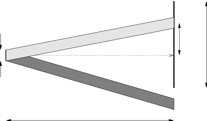
Fig. 2: A directed field propagates from a distributed source of size $\sigma_{s}$ toward the time reversal mirror of size $a$. The time-reversed, back-propagated field depends on the location of the mirror relative to the direction of the propagating beam.

For a distributed source, its support $\sigma_{s}$ is large compared to the Fresnel number $\theta$ so the ratio $\beta=\sigma_{s}/\theta$ is large. In this case we can compute the average of (40) the same way as we did in (41) and we find that

$$\langle\Psi^{B}(L,{\bf x}_{0},\xi,t)\rangle$$ (47)

$$=(2\pi)^{d}e^{i({\bf p}_{0}\cdot\xi-k_{0}c_{0}t)}\psi_{0}({\xi}/{\beta})\int\langle W(L,{\bf x}_{0},\frac{{\bf p}_{0}}{k_{0}+k})\rangle e^{-ikc_{0}t}\hat{g}(-c_{0}k)\frac{c_{0}dk}{2\pi}$$

$$=e^{i({\bf p}_{0}\cdot\xi-k_{0}c_{0}t)}\psi_{0}({\xi}/{\beta})\int\frac{d{\bf y}d{\bf w}c_{0}dk}{(2\pi)^{d+1}}\chi_{A}({\bf y})e^{i(\frac{L{\bf w}{\bf p}_{0}}{k_{0}+k}-{\bf w}\cdot{\bf y}-kc_{0}t)}e^{-\frac{DL^{3}w^{2}}{6}}\hat{g}(-c_{0}k).$$

The ${\bf y}$ integral on the right gives the Fourier transform of the aperture function $\chi_{A}({\bf y})$ so with $\omega_{0}=c_{0}k_{0}$ and a change of variable from $k$ to $\omega=c_{0}k$ we have

$$\langle\Psi^{B}(L,{\bf x}_{0},\xi,t)\rangle$$ (48)

$$=e^{i({\bf p}_{0}\cdot\xi-\omega_{0}t)}\psi_{0}({\xi}/{\beta})\int\frac{d\omega}{2\pi}e^{-i\omega t}\hat{g}(-\omega)~{}\chi_{A}*\left(\frac{e^{-x^{2}/(2a_{e}^{2})}}{(2\pi a_{e}^{2})^{d/2}}\right)(\frac{Lc_{0}{\bf p}_{0}}{\omega_{0}+\omega})$$

Here the star denotes convolution with respect to the spatial variables ${\bf x}$, and $a_{e}$ is the effective aperture defined by (46).

When multipathing is weak we can ignore the Gaussian factor in the convolution and we have

$$\langle\Psi^{B}(L,{\bf x}_{0},\xi,t)\rangle$$ (49)

$$=e^{i({\bf p}_{0}\cdot\xi-\omega_{0}t)}\psi_{0}({\xi}/{\beta})\int\frac{d\omega}{2\pi}e^{-i\omega t}\hat{g}(-\omega)~{}\chi_{A}\left(\frac{Lc_{0}{\bf p}_{0}}{\omega_{0}+\omega}\right)$$

In the opposite case, when there is strong multipathing and the effective aperture is much larger than the physical one, $a_{e}\gg a$, we have

$$\langle\Psi^{B}(L,{\bf x}_{0},\xi,t)\rangle$$ (50)

$$=e^{i({\bf p}_{0}\cdot\xi-\omega_{0}t)}\psi_{0}({\xi}/{\beta})\left(\frac{a}{\sqrt{2\pi}a_{e}}\right)^{d}\int\frac{d\omega}{2\pi}e^{-i\omega t}\hat{g}(-\omega){e^{-\frac{1}{2}(\frac{Lc_{0}{\bf p}_{0}}{a_{e}(\omega_{0}+\omega)})^{2}}}$$

To interpret these results we note first that a distributed source function of the form (44) can be considered as a phased array emitting an inhomogeneous plane wave, a beam, in the direction $(k,{\bf p}_{0})$, within the paraxial or parabolic approximation. The ratio $|{\bf p}_{0}|/k$ is the tangent of the angle the direction vector makes with the $z$ axis, and $L|{\bf p}_{0}|/k$ is the transverse distance of the beam center to the center of the phased array (see Figure 2). If for each $\omega$ the beam displacement vector $Lc_{0}{\bf p}_{0}/(\omega_{0}+\omega)$ is inside the set $A$ occupied by the time reversal array, then we recover at the source the full pulse in (49), time-reversed,

$$\langle\Psi^{B}(L,{\bf x}_{0},\xi,t)\rangle=e^{i({\bf p}_{0}\cdot\xi-\omega_{0}t)}\psi_{0}({\xi}/{\beta})g(-t).$$

If, however, for some frequencies the transverse displacement vector is outside the time reversal array, these frequencies will be nulled in the integration and a distorted time pulse will be received at the source. Depending on the position of the time reversal mirror relative to the beam, high or low frequencies may be nulled.

In a strongly multipathing medium the situation is quite different because the expression (50), or more generally (48), holds now. Even if the beam from the phased array does not intercept the time reversal mirror at all, we will still get a time reversed signal at the source but with a much diminished amplitude. If the beam falls entirely within the time reversal mirror then the time reversed pulse will be a distorted form of $g(-t)$, with its amplitude reduced by the factor $(a/a_{e})^{d}$. An interesting and important application of the time reversal of a beam in a random medium is the possibility of estimating the effective aperture $a_{e}$ by pointing the beam in different directions toward the time reversal mirror, measuring the time reversed signal that back propagates to the source, that is, to the phased array, and inferring $a_{e}$ by fitting the measurements to (48).

4 Summary and conclusions

We have analyzed and explained two important phenomena associated with time reversal in a random medium:

• Super-resolution of the back-propagated signal due to multipathing

• Self-averaging that gives a statistically stable refocusing

Our analysis is based on a specific asymptotic limit (see Section 2.1) where the longitudinal distance of propagation is much larger than the size of the time-reversal mirror, which in turn is much larger than the correlation length of the medium, fluctuations in the index of refraction are weak, and the wave length is short compared to the correlation length. This asymptotic regime is more relevant to optical or infrared time reversal than it is to sonar or ultrasound. We have related the self-averaging properties of the back-propagated signal to those of functionals of the Wigner distribution. Self-averaging of these functionals implies the statistical stability of the time-reversed and back-propagated signal in the frequency domain, provided that the source function is not too broad compared to the Fresnel number (12). Time reversal refocusing of waves emitted from a distributed source is self-averaging only in the time domain.

We apply our theoretical results about stochastic Wigner distributions to time reversal and discuss in detail super-resolution and statistical stability in section 3.

Appendix A The white noise limit and the parabolic approximation

We collect here some comments on the scaling analysis of section 2.1 and refer to [1, 27, 33] for additional comments and results on scaling and asymptotics in the high-frequency and white-noise regime.

The dimensionless parameters $\delta,\varepsilon,\gamma$ introduced by (10) in Section 2.1, along with the Fresnel number $\theta$ defined by (12), lead to the scaled parabolic wave equation (13). If we do not make the parabolic approximation and keep the $\psi_{zz}$ term we have the scaled Helmholtz equation, with the phase $e^{ikz}$ removed,

$$\frac{\varepsilon^{2}\theta^{2}}{\delta^{2}}\psi_{zz}+2ik\theta\psi_{z}+\theta^{2}\Delta_{\bf x}\psi+\frac{k^{2}\delta}{\varepsilon^{1/2}}\mu(\frac{{\bf x}}{\delta},\frac{z}{\varepsilon})\psi=0.$$ (51)

Here, as in (13), we relate the strength of the fluctuations $\sigma$ to $\varepsilon$ and $\delta$ by (14). Is the parabolic approximation valid in the ordering (15), $\theta\ll\varepsilon\ll\delta\ll 1$, that we have analyzed? The answer is yes but not before both $\theta$ and $\varepsilon$ limits have been taken, in which case the scaled Wigner distribution (16) converges to the Liouville-Ito process that is defined by the stochastic partial differential equation (27).

It is in the white noise limit $\varepsilon\to 0$, with Fresnel number $\theta$ and $\delta$ fixed, that the parabolic approximation is valid for (51), as was pointed out in [1]. This is easily seen if the random fluctuations $\mu$ are differentiable in $z$. The parabolic approximation is clearly not valid in the high frequency limit $\theta\to 0$, before the white noise limit $\varepsilon\to 0$ is also taken. In the white noise limit, the wave function $\psi(z,{\bf x})$ satisfies an Ito-Schrödinger equation

$$2ik\theta d_{z}\psi+\theta^{2}\Delta_{\bf x}\psi dz+\frac{ik^{3}\delta^{2}}{4\theta}R_{0}(0)\psi dz+k^{2}\delta\psi d_{z}B(\frac{{\bf x}}{\delta},z)=0.$$ (52)

Here $R_{0}$ is the integrated covariance of the fluctuations $\mu$ given by (23) and (21), and the Brownian field $B({\bf x},z)$ has covariance

$$\langle B({\bf x},z_{1})B({\bf y},z_{2})\rangle=R_{0}({\bf x}-{\bf y})z_{1}\wedge z_{2}.$$

This Ito-Schrödinger equation is the result of the central limit theorem applied to (51). Let

$$B^{\varepsilon}({\bf x},z)=\frac{1}{\sqrt{\varepsilon}}\int_{0}^{z}\mu({\bf x},\frac{s}{\varepsilon})ds.$$

Then, as $\varepsilon\to 0$ this process converges weakly, under suitable hypotheses, to the Brownian field $B({\bf x},z)$ with the above covariance. The extra term in (52) is the Stratonovich correction.

The white noise limit for stochastic partial differential equations is analyzed in [10] and a rigrous theory of the Ito-Schrödinger equation is given in [11]. The ergodic theory of the Ito-Schroedinger equation is explored in [17]. Wave propagation in the parabolic approximation with white-noise fluctuations is considered in detail in [18, 30].

The scaled Wigner distribution for the process $\psi$, defined by (16), satisfies the stochastic transport equation

$$d_{z}W_{\theta}(z,{\bf x},{\bf p})+\frac{{\bf p}}{k}\cdot\nabla_{x}W_{\theta}(z,{\bf x},{\bf p})dz$$ (53)

$$=\frac{k^{2}\delta^{2}}{4\theta^{2}}\int\frac{d{\bf q}}{(2\pi)^{d}}\hat{R}_{0}({\bf q})\left(W_{\theta}(z,{\bf x},{\bf p}+\frac{\theta{\bf q}}{\delta})-W_{\theta}(z,{\bf x},{\bf p})\right)dz$$

$$+\frac{ik\delta}{2\theta}\int\frac{d{\bf q}}{(2\pi)^{d}}e^{i{\bf q}\cdot{\bf x}/\delta}\left(W_{\theta}(z,{\bf x},{\bf p}-\frac{\theta{\bf q}}{2\delta})-W_{\theta}(z,{\bf x},{\bf p}+\frac{\theta{\bf q}}{2\delta})\right)d_{z}\hat{B}({\bf q},z),$$

which is derived from (52) equation using the Ito calculus. The Wigner process $W_{\theta}$ converges in the limit $\theta\to 0$ to the Liouville-Ito process defined by the stochastic partial differential equation (27).

Appendix B Decorrelation of the Wigner process

B.1 Proof of Theorem 1

We give here the proof of Theorems 1 and 2. We consider Theorem 1 first. It will follow from the Lebesgue dominated convergence theorem if we show that for ${\bf p}_{1}\neq{\bf p}_{2}$:

$$E\left\{W_{\delta}(z,{\bf x},{\bf p}_{1})W_{\delta}(z,{\bf x},{\bf p}_{2})\right\}-E\left\{W_{\delta}(z,{\bf x},{\bf p}_{1})\right\}E\left\{W_{\delta}(z,{\bf x},{\bf p}_{2})\right\}\to 0$$ (54)

as $\delta\to 0$ because the function $W_{\delta}$ is uniformly bounded and $E\left\{W_{\delta}(z,{\bf x},{\bf p}_{1})\right\}$ does not depend on $\delta$. Furthermore, the correlation function at the same spatial point but for two different values of the wave vector, $U_{\delta}^{(2)}(z,{\bf x},{\bf p}_{1},{\bf p}_{2})=E\left\{W_{\delta}(z,{\bf x},{\bf p}_{1})W_{\delta}(z,{\bf x},{\bf p}_{2})\right\}$ is the solution of (26) with $N=2$ and the initial data

$$W_{\delta}^{(2)}(0,{\bf x}_{1},{\bf p}_{1},{\bf x}_{2},{\bf p}_{2})=W_{I}({\bf x}_{1},{\bf p}_{1})W_{I}({\bf x}_{2},{\bf p}_{2}),$$

evaluated at ${\bf x}_{1}={\bf x}_{2}={\bf x}$. Therefore $U_{\delta}^{(2)}$ may be represented as

$$U_{\delta}^{(2)}(z,{\bf x}_{1},{\bf p}_{1},{\bf x}_{2},{\bf p}_{2})=E\left\{W_{I}({\bf X}_{\delta}^{1}(z),{\bf P}_{\delta}^{1}(z))W_{I}({\bf X}_{\delta}^{2}(z),{\bf P}_{\delta}^{2}(z))\right\}.$$

The processes ${\bf X}_{\delta}^{1,2}$ and ${\bf P}_{\delta}^{1,2}$ satisfy the system of SDE’s (24) which may be more explicitly written as

$$d{\bf P}_{\delta}^{1}=-\left[\sigma(0)d{\bf B}^{1}(z)+\frac{1}{2}\sigma\left(\frac{{\bf X}_{\delta}^{1}-{\bf X}_{\delta}^{2}}{\delta}\right)d{\bf B}^{2}(z)\right]$$ (55)

$$d{\bf P}_{\delta}^{2}=-\left[\sigma(0)d{\bf B}^{2}(z)+\frac{1}{2}\sigma\left(\frac{{\bf X}_{\delta}^{2}-{\bf X}_{\delta}^{1}}{\delta}\right)d{\bf B}^{1}(z)\right]$$

$$d{\bf X}_{\delta}^{1}=-{\bf P}_{\delta}^{1}dz,~{}~{}d{\bf X}_{\delta}^{2}=-{\bf P}_{\delta}^{2}dz$$

with the initial conditions ${\bf X}_{\delta}^{1,2}(0)={\bf x},~{}~{}{\bf P}_{\delta}^{m}(0)={\bf p}_{m}$, $m=1,2$. Here $\sigma^{2}(0)=D$, the diffusion coefficient (23) and the coupling matrix $\sigma({\bf x})$ is given by (25). Recall that $W_{\delta}(z,{\bf x},{\bf p},k)=W_{\delta}(z,{\bf x},{\bf p}/k;1)$ and we need only consider the case $k=1$.

It is convenient to introduce the processes ${\bf X}^{1,2}$ and ${\bf P}^{1,2}$ that are solutions of (24) with no coupling:

$$d{\bf P}^{m}=-\sigma(0)d{\bf B}^{m}(z),~{}~{}d{\bf X}^{m}=-{\bf P}^{m}dz,$$ (56)

$${\bf X}^{1,2}(0)={\bf x},~{}~{}{\bf P}^{m}(0)={\bf p}_{m},~{}~{}m=1,2$$

and define the deviations of the solutions of the coupled system of SDE’s (55) from those of (56): ${\bf Z}_{\delta}^{m}={\bf X}_{\delta}^{m}-{\bf X}^{m}$, ${\bf S}_{\delta}^{m}={\bf P}_{\delta}^{m}-{\bf P}^{m}$. Then we have

$$d{\bf S}_{\delta}^{1}=-\frac{1}{2}\sigma\left(\frac{{\bf X}_{\delta}^{1}-{\bf X}_{\delta}^{2}}{\delta}\right)d{\bf B}^{2}(z),~{}~{}d{\bf S}_{\delta}^{2}=-\frac{1}{2}\sigma\left(\frac{{\bf X}_{\delta}^{2}-{\bf X}_{\delta}^{1}}{\delta}\right)d{\bf B}^{1}(z)$$ (57)

$$d{\bf Z}_{\delta}^{1}=-{\bf S}_{\delta}^{1}dz,~{}~{}d{\bf Z}_{\delta}^{2}=-{\bf S}_{\delta}^{2}dz$$

with the initial data ${\bf S}_{\delta}^{m}(0)={\bf Z}^{m}(0)=0$. Define

$${\cal V}({\bf X}^{1},{\bf X}^{2},{\bf P}^{1},{\bf P}^{2},{\bf Z}^{1}_{\delta},{\bf Z}^{2}_{\delta},{\bf S}^{1}_{\delta},{\bf S}^{2}_{\delta})$$ (58)

$$=W_{I}({\bf X}^{1}+{\bf Z}_{\delta}^{1},{\bf P}^{1}+{\bf S}_{\delta}^{1})W_{I}({\bf X}^{2}+{\bf Z}_{\delta}^{2},{\bf P}^{2}+{\bf S}_{\delta}^{2})-W_{I}({\bf X}^{1},{\bf P}^{1})W_{I}({\bf X}^{2},{\bf P}^{2})$$

then we have with the above notation

$$E\left\{W_{\delta}(z,{\bf x},{\bf p}_{1})W_{\delta}(z,{\bf x},{\bf p}_{2})\right\}-E\left\{W_{\delta}(z,{\bf x},{\bf p}_{1})\right\}E\left\{W_{\delta}(z,{\bf x},{\bf p}_{2})\right\}$$ (59)

$$=E\left\{{\cal V}({\bf X}^{1}(z),{\bf X}^{2}(z),{\bf P}^{1}(z),{\bf P}^{2}(z),{\bf Z}^{1}_{\delta}(z),{\bf Z}^{2}_{\delta}(z),{\bf S}^{1}_{\delta}(z),{\bf S}^{2}_{\delta}(z))\right\}$$

$$\leq CE\left\{|{\bf Z}_{\delta}^{1}(z)|+|{\bf Z}_{\delta}^{2}(z)|+|{\bf S}_{\delta}^{1}(z)|+|{\bf S}_{\delta}^{2}(z)|\right\}$$

since $W_{I}$ is a Lipschitz function.

Let us assume for simplicity that the correlation function $R({\bf x})$ has compact support inside the set $|{\bf x}|\leq M$. Then the coupling term in (55) is non-zero only when $|{\bf X}_{\delta}^{1}-{\bf X}_{\delta}^{2}|\leq M\delta$. We introduce the processes ${\bf Q}_{\delta}={\bf P}_{\delta}^{1}-{\bf P}_{\delta}^{2}$ and ${\bf Y}_{\delta}={\bf X}_{\delta}^{1}-{\bf X}_{\delta}^{2}$ that govern (57). They satisfy the SDE’s

$$d{\bf Q}_{\delta}=-\left[\sigma(0)-\frac{1}{2}\sigma\left(\frac{{\bf Y}_{\delta}}{\delta}\right)\right]d\tilde{\bf B},~{}~{}d{\bf Y}_{\delta}=-{\bf Q}_{\delta}dz,$$ (60)

$$~{}~{}{\bf Q}_{\delta}(0)={\bf p}_{1}-{\bf p}_{2},~{}{\bf Y}_{\delta}(0)=0$$

with $\tilde{\bf B}={\bf B}^{1}-{\bf B}^{2}$ being a Brownian motion.

In order to prove the theorem we show that the coupling term $\sigma(\cdot)$ in (55) introduces only lower order correction terms, that is, ${\bf S}_{\delta}^{m}$ and ${\bf Z}_{\delta}^{m}$ are small. We show first that after a small ‘time’, $\tau$, the points ${\bf X}_{\delta}^{m}$ are driven apart since ${\bf Q}_{\delta}(0)={\bf P}_{\delta}^{1}(0)-{\bf P}_{\delta}^{2}(0)\neq 0$. Then we show that after the points have separated the probability that they come close, so that the coupling term $\sigma(\cdot)$ becomes non-zero, is small. This “non-recurrence” condition requires that the spatial dimension $d\geq 2$. It follows that to leading order the points ${\bf X}_{\delta}^{m}$ are uncorrelated when $d\geq 2$ and that the coupling term introduces only lower order corrections. A similar argument for $d=1$ would require an estimate on the time that points that are originally separated in the spatial variable spend near each other, where the coupling term in (55) is not zero.

We need the following two Lemmas. The first one shows that particles that start at the same point ${\bf x}$ with different initial directions ${\bf p}_{1}$ and ${\bf p}_{2}$, get separated with a large probability:

Lemma 3.

Let ${\bf Y}_{\delta}$, ${\bf Q}_{\delta}$ solve (60) with ${\bf Y}_{\delta}(0)=0$, ${\bf Q}_{\delta}(0)={\bf q}\neq 0$. Then for any $\varepsilon>0$ there exists $\tau_{0}(\varepsilon)>0$ that depends only on ${\bf q}={\bf p}_{1}-{\bf p}_{2}$ but not on $\delta$ so that we have $\displaystyle P\left(|{\bf Y}_{\delta}(\tau)|\geq\frac{|{\bf q}|\tau}{2}\right)\geq 1-\varepsilon$ for all $\tau\leq\tau_{0}(\varepsilon)$.

The second lemma shows that after the particles are separated, the probability that they come close to each other is small:

Lemma 4.

Given any fixed $r>0$ and $z>0$, if ${\bf Y}_{\delta}$, ${\bf Q}_{\delta}$ solve (60) with $|{\bf Y}_{\delta}(0)|\geq r$, ${\bf Q}_{\delta}(0)={\bf q}\neq 0$, then $P\left(\inf_{0\leq s\leq z}|{\bf Y}_{\delta}(s)|\leq M\delta\right)\to 0$ as $\delta\to 0$.

We prove Theorem 1 before proving Lemmas 3 and 4:

Proof.

Let $z$ and ${\bf q}={\bf p}_{1}-{\bf p}_{2}$ be fixed and defined as above. Given $\varepsilon>0$, then for any $\tau<\tau_{0}(\varepsilon)$ (with $\tau_{0}$ as defined in Lemma 3), Lemma 4 and the Markov property of the Brownian motion imply that

$$P\left({\bf S}_{\delta}^{m}(z)={\bf S}_{\delta}^{m}(\tau)\Big{|}|{\bf Y}_{\delta}(\tau)|\geq\frac{\tau|{\bf q}|}{2}\right)\geq 1-\varepsilon$$

and

$$P\left({\bf Z}_{\delta}^{m}(z)={\bf Z}_{\delta}^{m}(\tau)+(z-\tau){\bf S}_{\delta}^{m}(\tau)\Big{|}|{\bf Y}_{\delta}(\tau)|\geq\frac{\tau|{\bf q}|}{2}\right)\geq 1-\varepsilon$$

for $\delta<\delta_{0}(\tau,\varepsilon)$. Furthermore,

$$E\left\{|{\bf Z}_{\delta}^{1}(\tau)|+|{\bf Z}_{\delta}^{2}(\tau)|+|{\bf S}_{\delta}^{1}(\tau)|+|{\bf S}_{\delta}^{2}(\tau)|\Big{|}|{\bf Y}_{\delta}(\tau)|\geq\frac{\tau|{\bf q}|}{2}\right\}$$

$$\leq E\left\{|{\bf Z}_{\delta}^{1}(\tau)|+|{\bf Z}_{\delta}^{2}(\tau)|+|{\bf S}_{\delta}^{1}(\tau)|+|{\bf S}_{\delta}^{2}(\tau)|\right\}/(1-\varepsilon)\leq C\tau$$

because the function $\sigma$ is uniformly bounded. Therefore we have

$$~{}~{}~{}~{}~{}~{}~{}~{}~{}E\left\{{\cal V}({\bf X}^{1},{\bf X}^{2},{\bf P}^{1},{\bf P}^{2},{\bf Z}^{1}_{\delta},{\bf Z}^{2}_{\delta},{\bf S}^{1}_{\delta},{\bf S}^{2}_{\delta})\right\}$$

$$~{}~{}~{}~{}~{}~{}~{}~{}~{}=E\left\{{\cal V}({\bf X}^{1},{\bf X}^{2},{\bf P}^{1},{\bf P}^{2},{\bf Z}^{1}_{\delta},{\bf Z}^{2}_{\delta},{\bf S}^{1}_{\delta},{\bf S}^{2}_{\delta})\Big{|}|{\bf Y}_{\delta}(\tau)|\geq\frac{\tau|{\bf q}|}{2}\right\}P\left(|{\bf Y}_{\delta}(\tau)|\geq\frac{\tau|{\bf q}|}{2}\right)$$ (62)

$$+E\!\left\{{\cal V}({\bf X}^{1},{\bf X}^{2},{\bf P}^{1},{\bf P}^{2},{\bf Z}^{1}_{\delta},{\bf Z}^{2}_{\delta},{\bf S}^{1}_{\delta},{\bf S}^{2}_{\delta})\Big{|}|{\bf Y}_{\delta}(\tau)|\leq\frac{\tau|{\bf q}|}{2}\right\}P\left(\!|{\bf Y}_{\delta}(\tau)|\leq\frac{\tau|{\bf q}|}{2}\right)=I+II.$$

The second term above is small because the probability for ${\bf Y}_{\delta}(\tau)$ to be very small is bounded by Lemma 3. More precisely, given $\varepsilon>0$ and $\tau<\tau_{0}(\varepsilon)$, Lemma 3 implies that

$$II\leq C\varepsilon.$$ (63)

The first term in (62) corresponds to the more likely scenario that ${\bf Y}_{\delta}$ at time $\tau$ has left the ball of radius $\tau|{\bf q}|/2$. We estimate it as follows. The probability that ${\bf Y}_{\delta}$ re-enters the ball of radius $M\delta$ is small according to Lemma 4. Moreover, if ${\bf Y}_{\delta}$ stays outside this ball, the difference variables ${\bf Z}^{m}$ and ${\bf S}^{m}$ are bounded in terms of their values at time $\tau$. The latter are small if $\tau$ is small. More precisely, using (B.1) we choose $\tau$ so small that

$$E\left\{|{\bf Z}_{\delta}^{1}(\tau)|+|{\bf Z}_{\delta}^{2}(\tau)|+|{\bf S}_{\delta}^{1}(\tau)|+|{\bf S}_{\delta}^{2}(\tau)|\Big{|}|{\bf Y}_{\delta}(\tau)|\geq\frac{\tau|{\bf q}|}{2}\right\}\leq\varepsilon.$$

Then we obtain

$$I\leq E\left\{{\cal V}({\bf X}^{1},{\bf X}^{2},{\bf P}^{1},{\bf P}^{2},{\bf Z}^{1}_{\delta},{\bf Z}^{2}_{\delta},{\bf S}^{1}_{\delta},{\bf S}^{2}_{\delta})\Big{|}|{\bf Y}_{\delta}(\tau)|\geq\frac{\tau|{\bf q}|}{2}\right\}$$

$$\leq E\left\{{\cal V}({\bf X}^{1},{\bf X}^{2},{\bf P}^{1},{\bf P}^{2},{\bf Z}^{1}_{\delta},{\bf Z}^{2}_{\delta},{\bf S}^{1}_{\delta},{\bf S}^{2}_{\delta})\Big{|}|{\bf Y}_{\delta}(\tau)|\geq\frac{\tau|{\bf q}|}{2}\hbox{ and }\inf_{\tau\leq s\leq z}|{\bf Y}_{\delta}(s)|\leq M\delta\right\}$$

$$\times P\left(\inf_{\tau\leq s\leq z}|{\bf Y}_{\delta}(s)|\leq M\delta\Big{|}|{\bf Y}_{\delta}(\tau)|\geq\frac{\tau|{\bf q}|}{2}\right)$$

$$+E\left\{|{\bf Z}_{\delta}^{1}(z)|+|{\bf Z}_{\delta}^{2}(z)|+|{\bf S}_{\delta}^{1}(z)|+|{\bf S}_{\delta}^{2}(z)|\Big{|}|{\bf Y}_{\delta}(\tau)|\geq\frac{\tau|{\bf q}|}{2}\hbox{ and }\inf_{\tau\leq s\leq z}|{\bf Y}_{\delta}(s)|\geq M\delta\right\}$$

$$\times P\left(\inf_{\tau\leq s\leq z}|{\bf Y}_{\delta}(s)|\geq M\delta\Big{|}|{\bf Y}_{\delta}(\tau)|\geq\frac{\tau|{\bf q}|}{2}\right)=I_{1}+I_{2}.$$

The term $I_{1}$ goes to zero as $\delta\to 0$ by Lemma 4. However, if the conditions in $I_{2}$ hold, then

$${\bf S}_{\delta}^{m}(z)={\bf S}_{\delta}^{m}(\tau),~{}~{}{\bf Z}_{\delta}^{m}(z)={\bf Z}_{\delta}^{m}(\tau)-\frac{1}{k}(z-\tau){\bf S}_{\delta}^{m}(\tau).$$

Therefore the term $I_{2}$ may be bounded with the help of (B.1) by

$$I_{2}\leq E\left\{|{\bf Z}_{\delta}^{1}(z)|+|{\bf Z}_{\delta}^{2}(z)|+|{\bf S}_{\delta}^{1}(z)|+|{\bf S}_{\delta}^{2}(z)|\Big{|}|{\bf Y}_{\delta}(\tau)|\geq\frac{\tau|{\bf q}|}{2}\hbox{ and }\inf_{\tau\leq s\leq z}|{\bf Y}_{\delta}(s)|\geq M\delta\right\}$$

$$\leq CE\left\{|{\bf Z}_{\delta}^{1}(\tau)|+|{\bf Z}_{\delta}^{2}(\tau)|+|{\bf S}_{\delta}^{1}(\tau)|+|{\bf S}_{\delta}^{2}(\tau)|\Big{|}|{\bf Y}_{\delta}(\tau)|\geq\frac{\tau|{\bf q}|}{2}\right\}\leq C\tau.$$

Putting together (62), (63) and the above bounds on $I_{1}$ and $I_{2}$, we obtain

$$E\left\{|{\bf Z}_{\delta}^{1}(z)|+|{\bf Z}_{\delta}^{2}(z)|+|{\bf S}_{\delta}^{1}(z)|+|{\bf S}_{\delta}^{2}(z)|\right\}\leq C\varepsilon$$

for $\delta<\bar{\delta}$ and Theorem 1 follows from (59). ∎

B.2 Proof of Lemmas 3 and 4

We first prove Lemma 3.

Proof.

We write

$$Q_{\delta}(z)={\bf q}-\int_{0}^{z}\left(\sigma(0)-\frac{1}{2}\sigma({\bf Y}(s)/\delta)\right)~{}d\tilde{\bf B}(s)~{}\equiv~{}{\bf q}+\tilde{\bf Q}_{\delta}(z)$$

so that

$${\bf Y}_{\delta}(t)=-{\bf q}t-\int_{0}^{t}\tilde{\bf Q}_{\delta}(s)ds.$$

Then we have

$$P\left(\sup_{0\leq s\leq\tau}|\tilde{\bf Q}_{\delta}(s)|~{}>~{}r\right)\leq C\tau/r^{2}$$ (64)

and hence

$$P\left(|{\bf Y}_{\delta}(\tau)+\tau{\bf q}|>r\tau\right)\leq P\left(\sup_{0\leq s\leq\tau}|\tilde{\bf Q}_{\delta}(s)|>r\right)\leq C\tau/r^{2}.$$

We let $r=|{\bf q}|/2$ in the above formula and obtain

$$P\left(|{\bf Y}_{\delta}(\tau)|<\frac{\tau|{\bf q}|}{2}\right)\leq\frac{C}{|{\bf q}|^{2}}\tau,$$

and the conclusion of Lemma 3 follows. ∎

Finally, we prove Lemma 4.

Proof.

Let $\tau_{\delta}$ be the first time ${\bf Y}_{\delta}(z)$ enters the ball of radius $M\delta$:

$$\tau_{\delta}=\inf\left\{z:~{}|{\bf Y}_{\delta}(z)|\leq M\delta\right\},$$

with ${\bf Y}_{\delta}(0)={\bf Y}^{0}\neq 0$. For $0<\alpha<1$ let $\Delta z=\delta^{1-\alpha}$, $n=\lceil z/\Delta z\rceil$, $J_{i}=(i\Delta z,(i+1)\Delta z)$ and $p<1$. Note that until the time $\tau_{\delta}$ the process $({\bf Y}_{\delta},{\bf Q}_{\delta})$ coincides with the process $({\bf Y},{\bf Q})$ governed by (60) without the coupling term $\sigma({\bf Y}_{\delta}/\delta)$. We find

$$P(\tau_{\delta}<z)\leq\sum_{i=0}^{n-1}\left\{P\left(|{\bf Y}(i\Delta z)|<M\delta^{p}\right)+P\left(\inf_{s\in J_{i}}\!|{\bf Y}(s)|<M\delta~{}\Big{|}~{}|{\bf Y}(i\Delta z)|\geq M\delta^{p}\right)\right\}.$$

The process ${\bf Y}(s)$ is Gaussian with mean ${\bf Y}^{0}$ and variance ${\cal O}(s^{2})$. Therefore, there is a $\bar{\delta}>0$ such that for $\delta<\bar{\delta}$

$$P(|{\bf Y}(i\Delta z)|<M\delta^{p}) \leq C\delta^{dp}.$$

If we assume

$$p<1-\alpha$$ (65)

then also

$$P(\tau_{\delta}<z) \leq nC\left(\delta^{dp}+P\left(\sup_{0<s<\Delta z}|{\bf Y}(s)-{\bf Y}^{0}|\geq M[\delta^{p}-\delta]\right)\right)$$

$$\leq C(\delta^{dp+\alpha-1}+\delta^{\alpha-1}P\left(\sup_{0<s<\Delta z}|{\bf B}(s)|\geq M[\delta^{p}-\delta]/\Delta z\right))$$

$$\leq C(\delta^{dp+\alpha-1}+\delta^{\alpha-1}\frac{E\left\{{\bf B}(\Delta z)^{2r}\right\}\Delta z^{2r}}{(\delta^{p}-\delta)^{2r}})$$

$$\leq C\left[\delta^{dp+\alpha-1}+\delta^{\alpha-1-rp+3r(1-\alpha)/2}\right].$$

Note that with $p<1-\alpha$ and $r$ large enough, there is a $q>0$ so that

$$P(\tau_{\delta}<z)\leq C\delta^{q}$$

if $d\geq 2$ and Lemma 4 follows. ∎

B.3 Proof of Theorem 2

We need to show first that

$$J_{\delta}(z,{\bf x})=\int W_{\delta}(z,{\bf x},{\bf p})d{\bf p}$$ (66)

is finite with probability one. The stochastic flow $({\bf X}_{\delta}(t,{\bf x},{\bf p}),{\bf P}_{\delta}(t,{\bf x},{\bf p})$ is continuous in $(t,{\bf x},{\bf p})$ with probability one, so $W_{\delta}(z,{\bf x},{\bf p})=W_{I}({\bf X}_{\delta}(t,{\bf x},{\bf p}),{\bf P}_{\delta}(t,{\bf x},{\bf p}))$ is bounded and continuous. It is, moreover, non-negative if $W_{I}\geq 0$. We know that

$$\int E\{W_{\delta}(z,{\bf x},{\bf p})\}d{\bf p}$$

is finite and independent of $\delta$, and the order of integration and expectation can be interchanged by Tonelli’s theorem. This theorem implies in addition that $J_{\delta}(z,{\bf x})$ is finite with probability one.

We can now consider

$$E\{J_{\delta}^{2}(z,{\bf x})\}=\int E\{W_{\delta}(z,{\bf x},{\bf p}_{1})W_{\delta}(z,{\bf x},{\bf p}_{2})\}d{\bf p}_{1}d{\bf p}_{2}.$$

The integrand is bounded by an integrable function uniformly in $\delta$ because

$$E\{W_{\delta}(z,{\bf x},{\bf p}_{1})W_{\delta}(z,{\bf x},{\bf p}_{2})\}\leq E^{1/2}\{W_{\delta}^{2}(z,{\bf x},{\bf p}_{1})\}E^{1/2}\{W_{\delta}(z,{\bf x},{\bf p}_{2})\},$$

the right side does not depend on $\delta$, and is integrable. Therefore by the Lebesgue dominated convergence theorem and the results of the previous Section we have that

$$\lim_{\delta\to 0}E\{J_{\delta}^{2}(z,{\bf x})\}=E^{2}\{J_{\delta}(z,{\bf x})\}$$

and the right side does not depend on $\delta$. This completes the proof of Theorem 2.

References

• [1] F. Bailly, J.F. Clouet and J.P. Fouque, Parabolic and white noise approximation for waves in random media, SIAM Journal on Applied Mathematics 56, 1996, 1445-1470.
• [2] G.Bal and L. Ryzhik, Time reversal for classical waves in random media, Comptes rendus de l’Académie des sciences - Série I - Mathématique, 333, 2001, 1041-1046.
• [3] G.Bal and L. Ryzhik, Time reversal for waves in random media, Preprint, 2002.
• [4] G.Bal, G. Papanicolaou and L. Ryzhik, Self-averaging in time reversal for the parabolic wave equation Preprint, 2002.
• [5] G.Bal, G. Papanicolaou and L. Ryzhik, Radiative transport limit for the random Schrödinger equation, Nonlinearity, 15, 2002, 513-529.
• [6] G. Blankenship and G. C. Papanicolaou, Stability and Control of Stochastic Systems with Wide-Band Noise Disturbances, SIAM J. Appl. Math., 34, 1978, 437-476.
• [7] P. Blomgren, G. Papanicolaou, and H. Zhao, Super-Resolution in Time-Reversal Acoustics, J. Acoust. Soc. Am., 111, 2002, 230-248.
• [8] L. Borcea, C. Tsogka, G. Papanicolaou and J. Berryman, Imaging and time reversal in random media, to appear in Inverse Problems, 2002.
• [9] J. Berryman, L. Borcea, G. Papanicolaou and C. Tsogka, Statistically stable ultrasonic imaging in random media, Preprint, 2002.
• [10] R. Bouc and E. Pardoux, Asymptotic analysis of PDEs with wide-band noise disturbances and expansion of the moments, Stochastic Analysis and Applications, 2, 1984, 369-422.
• [11] D. Dawson and G. Papanicolaou, A random wave process, Appl. Math. Optim., 12, 1984, 97–114.
• [12] D. Dowling and D. Jackson, Phase conjugation in underwater acoustics, Jour. Acoust. Soc. Am., 89, 1990, 171-181
• [13] D. Dowling and D. Jackson, Narrow-band performance of phase-conjugate arrays in dynamic random media, Jour. Acoust. Soc. Am.,91, 1992, 3257-3277.
• [14] M. Fink and J. de Rosny, Time-reversed acoustics in random media and in chaotic cavities, Nonlinearity, 15, 2002, R1-R18.
• [15] M. Fink, D. Cassereau, A. Derode, C. Prada, P. Roux, M. Tanter, J.L. Thomas and F. Wu, Time-reversed acoustics, Rep. Progr. Phys., 63, 2000, 1933-1995.
• [16] M. Fink and C. Prada, Acoustic time-reversal mirrors, Inverse Problems, 17, 2001, R1–R38.
• [17] J.P. Fouque, G.C. Papanicolaou and Y. Samuelides, Forward and Markov Approximation: The Strong Intensity Fluctuations Regime Revisited, Waves in Random Media, 8, 1998, 303-314.
• [18] K. Furutsu, Random Media and Boundaries: Unified Theory, Two-Scale Method, and Applications, Springer Verlag, 1993.
• [19] P.Gérard, P.Markovich, N.Mauser and F.Poupaud, Homogenization limits and Wigner transforms, Comm.Pure Appl. Math., 50, 1997, 323-380.
• [20] W. Hodgkiss, H. Song, W. Kuperman, T. Akal, C. Ferla and D. Jackson, A long-range and variable focus phase-conjugation experiment in a shallow water, Jour. Acoust. Soc. Am., 105, 1999, 1597-1604.
• [21] H. Kesten and G. Papanicolaou, A Limit Theorem for Turbulent Diffusion, Comm. Math. Phys., 65, 1979, 97-128.
• [22] G. Papanicolaou and W. Kohler, Asymptotic analysis of deterministic and stochastic equations with rapidly varying components, Comm. Math. Phys. 45, 217–232, 1975.
• [23] H. Kunita, Stochastic flows and stochastic differential equations. Cambridge Studies in Advanced Mathematics, 24. Cambridge University Press, Cambridge, 1997.
• [24] W. Kuperman, W. Hodgkiss, H. Song, T. Akal, C. Ferla and D. Jackson, Phase-conjugation in the ocean, Jour. Acoust. Soc. Am., 102, 1997, 1-16.
• [25] W. Kuperman, W. Hodgkiss, H. Song, T. Akal, C. Ferla and D. Jackson, Phase conjugation in the ocean: Experimental demonstration of an acoustic time reversal mirror, J. Acoust. Soc. Am., 103, 1998, 25-40.
• [26] H. Kushner, Approximation and weak convergence methods for random processes, with applications to stochastic systems theory, MIT Press Series in Signal Processing, Optimization, and Control, MIT Press, 1984.
• [27] B. Nair and B. White, High-frequency wave propagation in random media- a unified approach, SIAM J. Appl. Math., 51, 1991, 374-411.
• [28] L. Ryzhik, G. Papanicolaou, and J. B. Keller. Transport equations for elastic and other waves in random media, Wave Motion, 24, 327–370, 1996.
• [29] F. Tappert, The parabolic approximation method, Lecture notes in physics, vol. 70, Wave propagation and underwater acoustics, Springer-Verlag, 1977.
• [30] V. I. Tatarskii, A. Ishimaru and V. U. Zavorotny, editors, Wave Propagation in Random Media (Scintillation), SPIE and IOP, 1993.
• [31] Thomas J. L. and M. Fink, Ultrasonic beam focusing through tissue inhomogeneities with a time reversal mirror: Application to transskull therapy, IEEE Trans. on Ultrasonics, Ferroelectrics and Frequency Control, Vol. 43, 1122-1129, (1996).
• [32] C. Tsogka and G. Papanicolaou, Time reversal through a solid-liquid interface and super-resolution, Preprint, 2001.
• [33] B. White, The stochastic caustic, SIAM Jour. Appl. Math., 44, 1984, 127-149.