Dynamic linear response of the SK spin glass coupled microscopically to a bath

Abstract

The dynamic linear response theory of a general Ising model weakly coupled to a heat bath is derived employing the quantum statistical theory of Mori, treating the Hamiltonian of the spin bath coupling as a perturbation, and applying the Markovian approximation. Both the dynamic susceptibility and the relaxation function are expressed in terms of the static susceptibility and the static internal field distribution function. For the special case of the SK spin glass this internal field distribution can be related to the solutions of the TAP equations in the entire temperature region. Application of this new relation and the use of numerical solutions of the modified TAP equations leads for finite but large systems to explicit results for the distribution function and for dynamic linear response functions. A detailed discussion is presented which includes finite-size effects. Due to the derived temperature dependence of the Onsager-Casimir coefficients a frequency-dependent shift of the cusp temperature of the real part of the dynamic susceptibility is found.

1 Introduction

The Ising model of Sherrington-Kirkpatrick (SK) [1] with quenched random bonds is the most important representative of a class of long-ranged models all describing spin glasses (for general references see [2, 3, 4]). For the static analysis of this model two complementary but conceptually different approaches exist. The first approach uses the replica method [1] and the breaking of the replica symmetry [5] to calculate bond-averaged quantities. The approach of Thouless-Anderson-Palmer (TAP) [6] is based on more conventional techniques and does not perform this bond average as it is expected that macroscopic physical quantities will be independent of the particular configuration in the thermodynamic limit.

Although the TAP equations are well established [2, 3, 7] they are still a field of current interest. It is suspected that not all aspects of this approach have yet been worked out. Recently the author [8] has reanalyzed the stability of these equations and has shown that unstable states cannot be described by the original TAP equations. Therefore he proposed modified TAP equations which turned out to be useful for explicit numerical calculations of the characteristic features of the SK model of finite-sizes [9].

Dynamical questions are of great importance for the physics of spin glasses (for reviews see [2, 3, 4]). Therefore numerous dynamical extensions have been added to the SK model. Following the early dynamical approaches [1, 10] Glauber dynamics has been used by various authors [8, 11, 12]. In addition, Langevin dynamics has been employed in the studies [13] mostly for the soft spin version of the SK model. Both the Langevin and the Glauber dynamics are basically phenomenological and can at best be justified partially by microscopic arguments. Note this also applies to the work of Szamel [12] although this approach is formulated in the ‘spirit’ of the microscopic Mori theory.

It is the aim of this paper to present a compete microscopic analysis of the dynamical linear response for the SK model coupled to a bath. An adequate tool for this purpose is the general theory of Mori [14, 15]. This quantum-statistical approach is used in the present work and is worked out not only for the SK model but for a general Ising model. Such a treatment is obvious and straightforward. Nevertheless, to the authors knowledge it has previously not been published .

As usual the results of the Mori theory are expressed in terms of static equilibrium quantities. Together with the static isothermal susceptibility, it is the internal field distribution function [18, 19] which fully determines the dynamical linear response. At this point we restrict the approach to the SK model. It is shown that the internal field distribution function can be related to the solutions of the TAP equations. Employing the approximate TAP solutions [9], all the quantities of the linear response theory can be numerically calculated in the entire temperature regime for all external fields.

The references [18, 19] showed that an exact and complete description of the thermodynamics of Ising models can be formulated in terms of the internal field distribution function. Thus as a byproduct the presented results of this function are of some interest independent of the dynamical linear response problems.

Following a description of the microscopic Hamiltonian, the Mori approach for a general Ising system is performed in section 2. The internal magnetic field distribution function for the SK model is treated in section 3. Both the analytical and numerical results for the field distribution function, the dynamic susceptibility and the response function are explicitly presented in section 4. Finally, some concluding remarks can be found in section 5.

2 Linear response for a general Ising system

2.1 The microscopic system

A system of $N$ spins $\bi{s}_{i}$ with $s={1\over 2}$ is considered in the presence of external fields $H_{i}$. The spins interact via an arbitrary Ising spin-spin interaction $J_{ij}(=J_{ji})$ and are described by the spin Hamiltonian

$${\cal H}^{S}=-\frac{1}{2}\sum_{i,j}J_{ij}S_{i}S_{j}-\sum_{i}H_{i}S_{i}=-2\sum_{i,j}J_{ij}s_{i}^{z}s_{j}^{z}-2\sum_{i}H_{i}s^{z}_{i}$$ (1)

where $J_{ii}=0$ is presumed. Both quantum spin $1\over 2$ operators $s_{i}^{z}$ and Ising spins $S_{i}(=2s_{i}^{z})$ are used simultaneously in this work. Note that at this stage the bonds $J_{ij}$ are quite general.

The assembly of spins is weakly coupled to a bath described by the Hamiltonian ${\cal H}^{B}$ via a spin bath interaction

$${\cal H}^{SB}=\sum_{i}\bi{B}_{i}\bi{s}_{i}=\sum_{i}\,\frac{1}{2}(B^{+}_{i}s^{-}_{i}\,+\,B^{-}_{i}s^{+}_{i})\,+\,B^{z}_{i}s^{z}_{i}$$ (2)

where the operators $\bi{B}_{i}$ represent variables of the bath system. Thus the total Hamiltonian is given by

$${\cal H}={\cal H}^{0}+{\cal H}^{SB}\quad\textrm{with}\quad{\cal H}^{0}={\cal H}^{B}+{\cal H}^{S}.$$ (3)

There is no need for an explicit specification of the bath Hamiltonian ${\cal H}^{B}$ and the bath operators $\bi{B}_{i}$. As shown below it is just the absorptive part $\chi_{B}^{\prime\prime}(\omega)$ of the dynamic bath susceptibility

$$\chi_{B}(\omega)=\chi_{B}^{\prime}(\omega)+i\chi_{B}^{\prime\prime}(\omega)=-i\int_{0}^{\infty}\langle[\,B^{-}_{i},e^{i\mathrm{L}^{B}\,t}B^{+}_{i}\,]\rangle_{(B)}\;e^{i\omega t}\mathrm{d}t\quad,$$ (4)

which enters the calculation and which is assumed to be known. In equation (4) $\langle\ldots\rangle_{(B)}$ represents the canonical thermal expectation value with respect to ${\cal H}^{B}$ and $\mathrm{L}^{B}$ denotes the Liouville operator defined by $\mathrm{L}^{B}A=[{\cal H}^{B},A]$ . For later use it is noted that $\chi_{B}^{\prime\prime}(\omega)$ may be rewritten as

$$\chi_{B}^{\prime\prime}(\omega)=\pm\,\pi\,(e^{\pm\beta\omega}-1)\;\langle B_{i}^{\mp}\,\delta(\mathrm{L}^{B}\pm\omega)\,B_{i}^{\pm}\rangle_{(B)}$$ (5)

which can easily be shown or can be found in literature [15]. In writing equation (4), it is assumed that the bath susceptibilities do not depend on the site $i$. This assumption is not essential and an extension to the general case is straightforward.

Let $\tau_{B}$ and $\tau_{S}$ be the relaxation times of the bath and the spin system respectively. Then it is natural to assume a fast relaxation to thermal equilibrium for the bath system compared to the spin system which implies

$$\tau_{B}\ll\tau_{S}\quad.$$ (6)

For the explicit determination of linear response quantities (see section 4.) the bath susceptibility $\chi_{B}^{\prime\prime}(\omega)$ enters for $\omega\tau_{S}\approx 1$. This implies $\omega\tau_{B}\ll 1$ and

$$\chi_{B}^{\prime\prime}(\omega)\approx\textrm{const}\;\omega\quad\textrm{for}\quad\omega\ll\tau_{B}^{-1}$$ (7)

can be used in the generic case for the explicit calculations of below. If the simple form $\chi_{B}(\omega)=\chi_{B}(1-i\omega/\tau_{B})$ is presumed, the constant of proportionality is given by const$=\chi_{B}/\tau_{B}$, which may in principle be temperature dependent. This dependence is neglected in this work by assuming a slow variation on scale determined by the spin glass temperature. This assumption is to a certain extent arbitrary but can be justified for special cases. Such a case is the Korringa mechanism, where the bath and the $\bi{B}_{i}$ are identified as the conduction electrons and itinerant spin density operators respectively.

2.2 Mori formalism for the dynamic susceptibility

The linear response of the magnetizations

$$\langle S_{i}\rangle(t)-\langle S_{i}\rangle=\sum_{j}\chi_{ij}(\omega)h_{j}^{ex}\exp{i\omega t}\quad,\quad t\geq 0$$ (8)

due to small time dependent external fields $h_{i}^{ex}\,\Theta(t)\exp{i\omega t}$ is governed by the dynamic susceptibility matrix $\boldsymbol{\chi}(\omega)$ which is given by the Kubo formula written in the Liouville space [14, 15]

$$\chi_{ij}(\omega)=\beta\big{(}\tilde{S}_{i}\big{|}\,\textrm{L}\,\{\textrm{L}+\omega+i\eta\}^{-1}\big{|}\,\tilde{S}_{j}\big{)}\quad,\quad\eta\rightarrow+0$$ (9)

with $\tilde{A}=A-\langle A\rangle$. In the Liouville space the operators $A$ of the state space are considered as vectors $|A)$ with the temperature dependent Mori scalar product

$$(A|B)=\frac{1}{\beta}\int_{0}^{\beta}\textrm{d}\lambda\langle A^{\dagger}e^{-\lambda{\cal H}}Be^{\lambda{\cal H}}\rangle=\frac{1}{\beta}\langle A^{\dagger}(1-e^{-\beta\mathrm{L}})\textrm{L}^{-1}B\rangle$$ (10)

where $\langle\ldots\rangle$ is the canonical thermal expectation value with respect to ${\cal H}$. Operators in the Liouville space like the Liouville operator

$$\textrm{L}|A)=|[{\cal H},A])$$ (11)

will be written in Roman letters .

Introducing the projection operator in Liouville space

$$\textrm{P}=\beta\sum_{ij}\big{|}\,\tilde{S}_{i}\big{)}\chi^{-1}_{ij}\big{(}\tilde{S}_{j}\big{|}\quad\textrm{with}\quad\chi_{ij}=\beta\big{(}\tilde{S}_{i}\big{|}\,\tilde{S}_{j}\big{)}$$ (12)

and applying the standard Mori projection procedure [14, 15] leads to

$$\boldsymbol{\chi}^{-1}(\omega)=\boldsymbol{\chi}^{-1}-i\omega\beta^{-1}\bi{L}^{-1}(\omega)\quad$$ (13)

with

$$L_{ij}(\omega)=L^{\prime}_{ij}(\omega)\,+iL^{\prime\prime}_{ij}(\omega)=i\big{(}S_{i}\big{|}\,\textrm{LQ}\,\{\textrm{QLQ}+\omega+i\eta\}^{-1}\textrm{QL}\big{|}\,S_{j}\big{)}$$ (14)

and with $\textrm{Q}=\textrm{1}-\textrm{P}$. The matrices $\boldsymbol{\chi}$ and $\bi{L}$ represent the static isothermal susceptibility matrix and the dynamic Onsager-Casimir matrix respectively. Note that the vectors $\big{|}\,\tilde{S}_{i}\big{)}$ which span the subspace P commute. Thus the frequency matrix vanishes in the present case.

According to the standard approach [15] for a sufficiently weak coupling ${\cal H}^{SB}$ the Markovian approximation $\bi{L}(\omega)\approx\bi{L}^{\prime}(0)$ can be applied in equation (13). Furthermore the leading order perturbation-theory expressions can be used for both $\boldsymbol{\chi}$ and $\bi{L}^{\prime}(0)$ in (13). The static isothermal susceptibility matrix is of the order zero and approximated by

$$\chi_{ij}=\beta\;\langle\tilde{S}_{i}\,\tilde{S}_{j}\rangle_{(S)}=\beta\;(\langle S_{i}\,S_{j}\rangle_{(S)}-m_{i}m_{j})$$ (15)

where $m_{i}=\langle S_{i}\rangle_{(S)}$ and where $\langle\ldots\rangle_{(S)}$ is the canonical thermal expectation value with respect to the Ising Hamiltonian (1).

Setting $\bi{L}=\bi{L}^{\prime}(0)$ the lowest order of this matrix is the second order in the perturbation and is given by

$$L_{ij}=\pi\;\big{(}\textrm{Q}^{0}\textrm{L}^{SB}S_{i}\;\big{|}\,\;\delta(\;\textrm{Q}^{0}\textrm{L}^{0}\textrm{Q}^{0}\;)\;\textrm{Q}^{0}\textrm{L}^{SB}S_{j}\big{)}_{(0)}=\pi\;\big{(}\textrm{L}^{SB}S_{i}\;\big{|}\,\;\delta(\,\textrm{L}^{0}\,)\;\textrm{L}^{SB}S_{j}\big{)}_{(0)}$$ (16)

where $\textrm{L}^{SB}$ and $\textrm{L}^{0}$ are the Liouville operators related to ${\cal H}^{SB}$ and to ${\cal H}^{0}$ respectively. The index $(0)$ denotes the Mori product taken with ${\cal H}^{0}$ alone and the projector $\textrm{Q}^{0}$ is defined with the latter Mori product. The projector $\textrm{Q}^{0}$ drops out, since $S_{i}$ commutes with ${\cal H}^{0}$ and thus $(\tilde{S}_{i}|\textrm{L}^{SB}S_{j})=i\langle\,\tilde{S}_{j}\,[{\cal H}^{SB},S_{j}\,]\rangle_{(0)}=0$ holds, where in addition the second equation of (10) was used. Recalling $J_{ii}=0$, one finds that

$$\delta(\,\textrm{L}^{0}\,)\,B^{\pm}_{i}s^{\mp}_{i}=s^{\mp}_{i}\;\delta\big{(}\,\textrm{L}^{B}\,\pm 2H_{i}\,\pm 2X_{i}\big{)}\,B^{\pm}_{i}$$ (17)

where the operator of the internal field $X_{i}$ at the site $i$ is given by

$$X_{i}=\sum_{j}J_{ij}S_{j}\quad.$$ (18)

Using equation (17) we find $L_{ij}=L_{ii}\;\delta_{ij}$ with

$$L_{ii}=\frac{\pi}{2}\,\Big{\langle}(1-S_{i})\;B^{+}_{i}\delta(\textrm{L}^{B}-2H_{i}-2X_{i})\,B^{-}_{i}+(1+S_{i})\;B^{-}_{i}\delta(\textrm{L}^{B}+2H_{i}+2X_{i})\,B^{+}_{i}\Big{\rangle}_{(0)}\,.$$ (19)

Let $O$ be any operator in the unitary space of the spins not involving site $i$. Then

$$\langle\,S_{i}O\,\rangle_{(S)}=\Big{\langle}\;\frac{\;\textrm{Tr}_{i}S_{i}O\exp(-\beta H_{i}-\beta X_{i})}{\textrm{Tr}_{i}\;\exp(-\beta H_{i}-\beta X_{i})}\Big{\rangle}_{(S)}=\langle\,O\,\tanh\beta(H_{i}+X_{i})\,\rangle_{(S)}$$ (20)

can be obtained [19]. Applying this relation to equation (19) and using (5) finally yields for the dynamic susceptibility matrix

$$\boldsymbol{\chi}^{-1}(\omega)=\boldsymbol{\chi}^{-1}-i\omega(\beta\bi{L})^{-1}\quad\textrm{with}\quad L_{ij}=\delta_{ij}\,\,\Big{\langle}\;\frac{\chi_{B}^{\prime\prime}(2H_{i}+2X_{i})}{\sinh\beta(2H_{i}+2X_{i})}\;\Big{\rangle}_{(S)}$$ (21)

where the static isothermal susceptibility matrix $\boldsymbol{\chi}$ and the internal field operators $X_{i}$ are given by equation (15) and by equation (18) respectively.

To complete the analytic investigations for the general Ising case, the local-field probability distribution functions

$$P_{i}(h)\;=\langle\delta(h-H_{i}-X_{i})\rangle_{(S)}=\langle\delta(h-H_{i}-\Sigma_{j}\;J_{ij}S_{j})\rangle_{(S)}$$ (22)

are introduced which permits the $L_{ii}$ to be rewritten as

$$L_{ii}=\,\int\,P_{i}(h)\;\frac{\chi_{B}^{\prime\prime}(2h)}{\sinh(\beta 2h)}\,\mathrm{d}h\quad.$$ (23)

From the definition the relations

$$\int P_{i}(h)\,\mathrm{d}h=1\quad,\;\int h\,P_{i}(h)\,\mathrm{d}h=H_{i}+\sum_{j}J_{ij}m_{j}\quad,\quad\int\tanh(\beta h)\,P_{i}(h)\,\mathrm{d}h=m_{i}$$ (24)

immediately result, where the last relation is based on equation (20) with $O=1$.

With the result (21) we have found in a very compact form of the dynamic susceptibility matrix $\boldsymbol{\chi}(\omega)$ . This result is not restricted to the SK model and holds for all Ising models. According to the equations (21) and (23) the dynamic susceptibility $\boldsymbol{\chi}(\omega)$ can be explicitly calculated provided that the static susceptibility $\boldsymbol{\chi}$ and the internal magnetic field distribution functions $P_{i}(h)$ are known.

Knowledge of the linear dynamic susceptibility $\boldsymbol{\chi}(\omega)$ implies knowledge of all the other response functions. Let us consider the linear relaxation functions $\boldsymbol{\Phi}(t)$ which describe the linear response $\langle\tilde{S}_{i}\rangle(t)=\sum_{j}[\Phi_{ij}(t)-\chi_{ij}]\;h_{j}^{ex}$ for $t\geq 0$ due to small changes of the external fields $-h^{ex}_{j}\Theta(t)$. According to the general response theory $\boldsymbol{\Phi}(t)$ is given by

$$\Phi_{ij}(t)=\beta(\tilde{S}_{i}\big{|}\,\tilde{S}_{j}(t)\big{)}$$ (25)

and is approximated by

$$\frac{\textrm{d}\boldsymbol{\Phi}(t)}{\textrm{d}t}=-\beta\,{\bi{L}}\boldsymbol{\chi}^{-1}\,{\boldsymbol{\Phi}}(t)\quad\textrm{or by }\quad\boldsymbol{\Phi}(t)=\boldsymbol{\chi}\,\exp(-\boldsymbol{\chi}^{-1}\beta\,{\bi{L}}\,t)\quad.$$ (26)

The remaining quantity of interest in linear response theory is the response function matrix which equals $-\dot{\boldsymbol{\Phi}}(t)$. Due to this simple relation the response function matrix is not further considered in this work.

The results (26) can be compared in detail with the work of Szamel [12] which represents both the most recent and the closest treatment on the subject of this paper. Comparing equation (26) for the case $H_{i}=0$ with equation (13) of the first paper of reference [12] clearly shows that the values $(1-\langle S_{i}\tanh\beta X_{i}\rangle_{(S)})$ or according to relation (20) the values $(1-\langle\tanh^{2}\beta X_{i}\rangle_{(S)})$ are used for the $L_{ii}$ instead the correct values given in equation (21). Thus in general both approaches disagree.

The work of Szamel and other former work [11] is based on the phenomenological Glauber dynamics. Microscopic derivation [16, 17] of this master-equation (in the form of reference [12]) leads to the transition rates

$$w_{i}=(1-S_{i}\tanh\beta X_{i})\frac{\chi_{B}^{\prime\prime}(2X_{i})}{4\tanh\beta X_{i}}\quad$$ (27)

for the $H_{i}=0$ case. In the work of Szamel the values for the rates $(1-S_{i}\tanh\beta X_{i})/2$ were used which can only be justified for the special, rather unrealistic case that the bath susceptibility $\chi^{\prime\prime}_{B}(\omega)$ is proportional to $\tanh(\beta\omega/2)$. Thus, for a general agreement with the present approach, the correct transition rates (27) have to be used in the master-equation treatment.

Microscopically unjustified rates of the form of [12] are widely used to analyze the dynamics of Ising models for various physical questions. Provided the characteristic width of the distribution $P(h)$ is of the order of the temperature $T$ or larger than $T$ a modified master-equation approach with the rates (27) will lead to significant changes. Note that for (standard) mean field treatments these effects are absent. In these cases $P(h)$ is a $\delta$-function and the modifications reduce to a factor which can be eliminated by scaling the time. For the spin glasses at low temperatures, however, the exact form of the transition rates is essential, as worked out in the following for the SK model.

3 Internal field distribution function for the SK spin glass

For the rest of the paper we consider exclusively the special case of the SK model. In this case the bonds $J_{ij}$ are independent random variables with zero means and standard deviations $N^{-{1\over 2}}$. This scaling fixes the spin glass temperature to $T=1$. The smallness and the randomness enter basically into the approach of this section where a tractable form for the field distribution $P_{i}(x)$ of the SK model is deduced.

This approach uses techniques similar to the derivations of the TAP equations [6, 2, 8]. The spin Hamiltonian (1) is rewritten as ${\cal H}^{S}=-(H_{i}+X_{i})S_{i}+\hat{\cal H}_{i}$ where $\hat{\cal H}_{i}$ describes a $N-1$ spin system with the spin $S_{i}$ removed from the original spin system. Using the relation $\delta(h-H_{i}-X_{i})\exp[\beta(H_{i}+X_{i})S_{i}]=\delta(h-H_{i}-X_{i})\exp(\beta hS_{i})$ and the Fourier representation of the $\delta$-function and taking the trace over the site $i$

$$P_{i}(h)\;=\frac{\cosh(\beta h)}{i\pi Z}\int_{-\infty}^{\infty}\hat{Z}_{i}(k)\,e^{-ik(h-H_{i})}\,\textrm{d}k\quad\textrm{with}\quad\hat{Z}_{i}(k)=\hat{\Tr}_{i}\;e^{ik\sum_{j}J_{ij}S_{j}-\beta\hat{\cal H}_{i}}$$ (28)

is obtained. The partition function of the original spin system is denoted by $Z$ and $\hat{\Tr}_{i}$ stands for the trace of the $N-1$ spin system.

The quantity $\hat{Z}_{i}(k)$ represents a partition function of the $N-1$ spin system in presence of additional imaginary fields $ik\beta^{-1}J_{ij}$. Due to the smallness of the $J_{ij}$ the cumulant expansion can be performed which yields to leading order in $N^{-1}$ [6, 2, 8]

$$\ln\hat{Z}_{i}(k)=\ln\hat{Z}_{i}(0)+ik\sum_{j}J_{ij}\hat{m}_{j}-\frac{k^{2}}{2\beta}\sum_{j\,l}J_{ij}\hat{\chi}_{jl}J_{li}$$ (29)

where $\hat{m}_{j}=\beta^{-1}\partial\ln\hat{Z}_{i}(0)/\partial H_{j}$ and $\hat{\chi}_{jl}=\partial\hat{m}_{j}/\partial H_{l}$ are the local magnetizations and the static susceptibilities of the $N-1$ spin system respectively. Following again the former approaches [6, 2, 8] the double sum in equation (29) is replaced by the local static susceptibility

$$\chi_{l}=\frac{1}{N}\sum_{j}\chi_{jj}=\frac{1}{N}\sum_{j}\frac{\partial m_{j}}{\partial H_{j}}\quad.$$ (30)

With the result (29) the integration in equation (28) can be performed yielding

$$P_{i}(h)=\sqrt{\frac{\beta}{2\pi\chi_{l}}}\;\frac{\cosh(\beta h)}{\cosh(\beta H_{i}^{eff})}\;\exp\Big{\{}-\frac{\beta\chi_{l}}{2}\Big{\}}\;\exp\Big{\{}-\frac{\beta(h-H_{i}^{eff})^{2}}{2\chi_{l}}\Big{\}}$$ (31)

where the factors independent of $h$ are determined from the normalization condition $1=\int P_{i}(h)\,\textrm{d}h$ and where the local effective field $H_{i}^{eff}=H_{i}+\sum_{j}J_{ij}\hat{m}_{j}$ was introduced. The latter two relations of equation (24) yield

$$H_{i}^{eff}=H_{i}+\sum_{j}J_{ij}m_{j}-m_{j}\chi_{l}\quad\textrm{and}\quad m_{i}=\tanh(\beta H_{i}^{eff})$$ (32)

which is employed to rewrite equation (31) as function of $h,m_{i}$ and $\chi_{l}$

$$P_{i}(h)=\sqrt{\frac{\beta(1-m_{i}^{2})}{2\pi\chi_{l}}}\;\cosh(\beta h)\;\exp\Big{\{}-\frac{\beta\chi_{l}}{2}\Big{\}}\;\exp\Big{\{}-\frac{\beta(h-\beta^{-1}\mathrm{artanh}\>m_{i})^{2}}{2\chi_{l}}\Big{\}}\;.$$ (33)

Note that equation (32) are the well known TAP equations if the local static susceptibility $\chi_{l}$ is specified. In this work the modified version [8] of these equations is used which yields

$$\chi_{l}=\frac{1}{N}\sum_{i}\frac{\beta(1-m_{i}^{2})}{1+\Gamma^{2}\,\beta^{2}(1-m_{i}^{2})^{2}}$$ (34)

with

$$\Gamma=0\quad \mathrm{f} \mathrm{or}\quad 1-\frac{\beta^{2}}{N}\,\sum_{i}(1-m_{i}^{2})^{2}\geq 0$$ (35)

$$1=\frac{1}{N}\sum_{i}\frac{\beta^{2}(1-m_{i}^{2})^{2}}{1+\Gamma^{2}\,\beta^{2}(1-m_{i}^{2})^{2}}\qquad \mathrm{f} \mathrm{or}\quad 1-\frac{\beta^{2}}{N}\,\sum_{i}(1-m_{i}^{2})^{2}\leq 0\quad.$$ (36)

As worked out in [8], for the stable states the modified TAP equations are equivalent to the original ones in the thermodynamic limit and differences result only for unstable states. For finite systems the complete temperature and field dependence of the solutions of the modified equations is known [9], in contrast to the original TAP equations.

With the knowledge of these solutions the total internal field distribution function defined as

$$P(h)=\frac{1}{N}\sum_{i}\;P_{i}(h)$$ (37)

can be calculated according to equation (31) or (33). In zero field above the spin glass temperature the distribution function reduces to

$$P(h)=P_{i}(h)=\frac{1}{\sqrt{2\pi}}\;\cosh(\beta h)\;\exp\Big{\{}-\frac{\beta^{2}+h^{2}}{2}\Big{\}}\quad\textrm{for}\quad T\geq 1\;,\quad H_{i}=0\quad.$$ (38)

The latter result for the special case has already been obtained by Thomsen et al[19]. However, to the best of the authors knowledge, the general results of this section have previously not been published.

4 Discussion and numerical results

4.1 Internal field distribution function

The static properties of Ising models can entirely be formulated in terms of the internal field distribution function $P(h)$ [18, 19]. Due to this general importance some discussion of $P(h)$ for the SK model is presented.

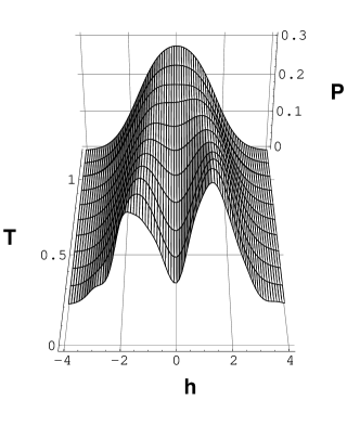
Figure 1: Temperature dependence of the internal field distribution function $P(h)$ of the SK spin glass for temperatures $T$ below and above the spin-glass temperature $T=1$ for zero external field.

For zero magnetic field the temperature dependence of $P(h)$ is shown in figure (1). Above the spin- glass temperature $T=1$ the exact result (38) is plotted. Below the spin glass temperature the figure is based on equation (33) and on the numerical results of [9]. In the plot the local magnetizations $m_{i}$ for the state of lowest free energy of a N=225 system (sample I) are used. On the scale of figure (1) both regimes $T\geq 1$ and $T\leq 1$ fit smoothly together. The distribution function $P(h)$ bifurcates from a one-peak structure to a two-peak structure at the spin-glass temperature. With decreasing temperature the minimum located at $h=0$ becomes deeper and finally reaches the value $P(h=0)=0$ for zero temperature within numeric precision. This behavior also applies to the metastable states. Moreover the variations for the different states are small and seem to become negligible in the thermodynamic limit. This is remarkable and is an indication for self averaging of $P(h)$. These findings, as well as the general temperature dependence of $P(h)$, are in agreement with Monte-Carlo simulations of references [19].

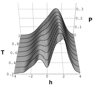
Figure 2: Temperature dependence of internal field distribution function $P(h)$ of the SK spin glass in presence of a homogenous external field H=0.5. The (numerical) AT temperature is T=.577 .

The discussion is completed by figure (2) where $P(h)$ is shown for a system with a homogenous external field $H=0.5$. No exact results are known for this case and thus the plot is based on numerical data everywhere. Again the data of sample I of reference [9] are used. Now the distribution $P(h)$ is asymmetric but again a bifurcation to a two-peak structure is found when the spin glass regime is entered. This occurs at the Almeida-Thouless (AT) temperature [20] which is determined from $T^{2}=N^{-1}\sum_{i}(1-m_{i}^{2})^{2}$ and which leads to the numerical value of $T=.577$ for the sample under consideration. These results indicate that the spin glass regime is also characterized by a two-peak structure of $P(h)$ for the case where a finite external field is present.

Certainly in the numerical results finite-size effects are present. The most obvious feature is the asymmetry of $P(h)$ in figure (1). Thus the investigations of the finite-size effects [9] are extended to the distribution function $P(h)$ and averages over a few tens of independent samples are performed keeping $N$ and $T$ fixed. For the averages the asymmetry of $P(h)$ for the case $H=0$ reduces both with increasing number of samples and with increasing $N$ . This represents some numerical evidence that the asymmetry is indeed an artifact due to the finite system size.

In this context we recall that in zero magnetic field for each solution of the TAP equation (32) a further solution can be constructed trivially by changing the sign of all $m_{i}$. According to equation (31) the distributions corresponding to these two solutions are given by $P(h)$ and by $P(-h)$ respectively. The means of these two distributions exhibit considerable smaller sample-to-sample variations than the individual $P(h)$. This can in principle be used to construct improved approximations of $P(h)$ for the thermodynamic limit. The TAP approach, however, does not use any averaging and thus we avoid this procedure. Moreover the asymmetry of figure (1) indicates the order of magnitude of the finite-size effects.

4.2 Dynamic susceptibility

We focus on the local dynamic susceptibility which is defined as

$$\chi_{l}(\omega)=\chi_{l}^{\prime}(\omega)+i\,\chi_{l}^{\prime\prime}(\omega)=N^{-1}\Tr\boldsymbol{\chi}(\omega)=N^{-1}\Tr\big{\{}\boldsymbol{\chi}^{-1}-i\omega(\beta{\bi L})^{-1}\big{\}}^{-1}$$ (39)

and which is a quantity of both theoretical and experimental interest. Employing the results of the last subsection and the approximation (7) (setting const=$1$ which fixes the time scale) the Onsager coefficient $L_{ii}$ can be numerically determined according to equation (23). Furthermore using the well known expression for the static isothermal susceptibility

$$\chi_{ij}^{-1}=\Big{\{}[\beta(1-m_{i}^{2})]^{-1}+\chi_{l}\Big{\}}\;\delta_{ij}-J_{ij}$$ (40)

with $\chi_{l}$ given by the equations (34-36), all terms of equation (21) are explicitly known and the dynamic susceptibility matrix $\boldsymbol{\chi}(\omega)$ is obtained by numerical matrix inversion. From this the local susceptibility $\chi_{l}(\omega)$ is finally calculated.

A further method exists to determine $\chi_{l}(\omega)$ which is based on the theorem of Pastur [21] . This theorem immediately leads to the identity (compare [8])

$$\chi_{l}(\omega)=N^{-1}\sum_{i}\big{\{}[\beta(1-m_{i}^{2})]^{-1}+\chi_{l}-i\omega(\beta L_{ii})^{-1}-\chi_{l}(\omega)\big{\}}^{-1}$$ (41)

and $\chi_{l}(\omega)$ is obtained as a solution of equation (41) satisfying $\omega\,\chi_{l}^{\prime\prime}(\omega)\geq 0$. In the paramagnetic regime and in absence of external magnetic fields this equation leads to the analytic result

$$\chi_{l}(\omega)=\frac{\beta+\beta^{-1}-i\omega\beta^{-1}L^{-1}}{2}+\sqrt{\frac{(\beta+\beta^{-1}-i\omega\beta^{-1}L^{-1})^{2}}{4}-1}\quad T\geq 1\;,\;H_{i}=0$$ (42)

where the Onsager coefficient $L_{ii}=L(T)$ is temperature dependent and given by

$$L(T)=\exp(-\beta^{2}/2)\frac{1}{\sqrt{2\pi}}\int\frac{h\,\exp(-h^{2}/2)}{\sinh\beta h}\;\textrm{d}h\quad.$$ (43)

using the equations (23) and (38). Note that for $T\gg 1$ equation (42) reduces to $\chi_{l}=\beta(1-i\omega\beta)^{-1}$ which implies a relaxation time proportional to $\beta$, as is the case for the Korringa relaxation of single magnetic moments dissolved in a metal. Note further that the result (42) partially agrees with the work of Kinzel and Fischer [10, 3] who, however, have not obtained the temperature dependence of $L(T)$. Near the spin glass temperature both approaches agree and yield $\chi_{l}(\omega)=1+i\sqrt{|\omega|}\,$ at $T=1$.

With reference to the definition of $\Gamma$ [8, 9]

$$\chi_{l}(\omega)\mid_{\omega\rightarrow\pm 0}=\chi_{l}\pm i\Gamma$$ (44)

results from equation (41). Thus the quantities $\chi_{l}$ and $\Gamma$, which enter formally in derivation the modified TAP equations, are related to the real and the imaginary part of the isolated susceptibility $\chi_{l}(\omega\rightarrow 0)$. Recalling that there are frequently situations in physics where the isolated and the isothermal susceptibility differ (for some general discussion see [15]) this result gives some additional insight into approach leading to the modified TAP equations [8, 9].

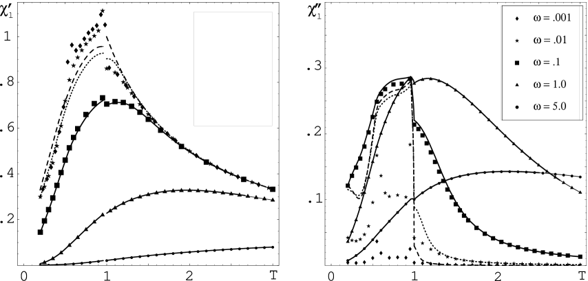
Figure 3: Temperature dependence of the real part, $\chi_{l}^{\prime}(\omega)$, and the imaginary part, $\chi_{l}^{\prime\prime}(\omega)$, of the local dynamic susceptibility $\chi_{l}(\omega)$ in zero external field for different frequencies. The data points are calculated by numerical inversion of equation (40) for a system of $N=225$ spins (compare text). The lines represent the results calculated from equation (41) via the theorem of Pastur. For $T<1$ they are again based on the numerical data of the $N=225$ spin system. For $T>1$ the lines give the analytic result of equation (42) in the thermodynamic limit. The dashed line, the dotted line and the full lines correspond to $\omega=0.001$, to $\omega=0.01$ and to $\omega=0.1,1.0,5.0$ respectively. For $\omega=0.001$ some data points exist which are outside the plot-range of $\chi_{l}^{\prime}(\omega)$.

In figure (3) both the analytical and the numerical results for $\chi_{l}$ are presented for the zero external field case. For the numerical parts again the lowest free energy state of sample I from reference [9] with $N=225$ is used. The two different methods lead to similar results but deviate increasingly for small frequencies $\omega$. It is remarkable that the results of figure (3) show some overall similarity to real, experimental data [3, 4]. One of these features is the frequency dependence of the cusp temperature of $\chi_{l}^{\prime}(T,\omega=const)$. In the present approach the shift results simply from the temperature dependence of the Onsager coefficients.

The deviations appearing in figure (3) for small frequencies are caused by the finite-size of the system. According to equation (21) $\bi{L}$ is positive definite. Thus the matrix $\bi{A}=(\beta\bi{L})^{1\over 2}$ is well defined and $\boldsymbol{\chi}^{-1}(\omega)$ can be rewritten as $\boldsymbol{\chi}^{-1}(\omega)=\bi{A}^{-1}(\bi{A}\boldsymbol{\chi}^{-1}\bi{A}-i\omega)\bi{A}^{-1}$. Use of the diagonal representation of $\bi{A}\boldsymbol{\chi}^{-1}\bi{A}$ leads to

$$\chi_{l}(\omega)=N^{-1}\sum_{\alpha}\langle u_{\alpha}|\bi{A}^{2}|u_{\alpha}\rangle\;(\delta_{\alpha}-i\omega)^{-1}\quad\textrm{where}\quad\bi{A}\boldsymbol{\chi}^{-1}\bi{A}|u_{\alpha}\rangle=\delta_{\alpha}|u_{\alpha}\rangle\>$$ (45)

which shows that $\chi_{l}(\omega)$ can be written as a superposition of Lorenzian functions with relaxation rates $\delta_{\alpha}$ given by the eigenvalues of $\bi{A}\boldsymbol{\chi}^{-1}\bi{A}$ . In the spin glass regime the minimum value $\delta_{min}$ of all rates $\delta_{\alpha}$ is small (the numerical value for the data used in figure (3) is of the order 0.03) for finite $N$ and tends to zero in the thermodynamic limit [8, 9, 22]. For frequencies $\omega<\delta_{min}$ the susceptibility $\chi_{l}(\omega)$ sensitively depends on the small eigenvalues according to equation (45) and thus finite-size effects mainly show up for small $\omega$ for the data obtained by direct matrix inversion. According to figure (3) the deviations are moderate for those results which use the theorem of Pastur. This indicates that the use of this theorem for finite $N$ smoothes partly out the finite-size effects.

4.3 Relaxation function

The local relaxation function can be written as

$$\Phi_{l}(t)=N^{-1}\Tr\boldsymbol{\Phi}(t)=N^{-1}\sum_{\alpha}\langle u_{\alpha}|\bi{A}^{2}|u_{\alpha}\rangle\;{\delta_{\alpha}}^{-1}\>\exp(-\delta_{\alpha}t)$$ (46)

where equation (26) and the eigenvalue equation (45) and were used. Again the superposition of the contributions resulting from the different rates $\delta_{\alpha}$ (or relaxation times $\delta_{\alpha}^{-1}$ ) can be identified. The local relaxation function satisfies $\Phi_{l}(t)\leq\Phi_{l}(0)=\chi_{l}.$ and thus is well behaved in the thermodynamic limit even for the case when $\delta_{min}$ tends to zero. For vanishing external fields $\Phi_{l}(t)$ can be given analytically

$$\Phi_{l}(t)=\frac{2}{\pi}\int_{-1}^{1}\,\textrm{d}x\frac{\sqrt{1-x^{2}}}{\beta+\beta^{-1}-2x}\exp\Big{[}-(1+\beta^{2}-2\beta x)L(T)\Big{]}\quad T\geq 1\;,\;H_{i}=0$$ (47)

in the paramagnetic regime [1]. As already noted, the temperature dependence of $L(T)$ differs from [1, 12] and is given by equation (43).

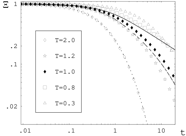
Figure 4: Time $t$ dependence of the reduced local relaxation function $\Xi(t)=\Phi_{l}(t)/\Phi_{l}(0)$ in a double log scale for different temperatures $T$ in zero external field. The data points correspond to the numerical results of a sample with $N=225$ spins. The lines represent the results in the thermodynamic limit given by equation (47). The full, the dashed and the dotted line correspond to $T=1.0,1.2$ , and $2.0$ respectively.

In figure (4) the numerical results for the local relaxation function $\Phi_{l}(t)$ are plotted (again for the state with lowest free energy of sample I of reference [9]) together the analytic results (47). The plot clearly exhibits the slowing down at the spin glass temperature and the presence of the slow dynamics in the spin glass regime. Comparing the numerical and the analytical results above the spin glass temperature the deviations increase for the long time behavior when approaching the spin glass regime. As discussed already above, these finite-size effects result from the finite value of $\delta_{min}$ and limits the numerical results to the region $t\ll\delta_{min}\approx 30$ near and below the spin glass temperature.

5 Conclusions

Two questions are studied from a more general point of view in the present work. First of all the linear response theory for an arbitrary Ising model which is microscopically and weakly coupled to a bath is investigated using the theory of Mori and applying the standard approximations. This approach seems to be natural and conservative and could have been carried out some decades ago. Nevertheless the results are remarkable, as the entire dynamical response of any Ising model is completely determined by the internal field distribution function, by the static isothermal susceptibility and - as the only characteristic feature of bath - by a bath dynamic susceptibility. Due to the simple structure this part of the present work may be of interest for other models than the SK model.

The relation to former approaches has been worked out in some detail at the end of section 2. It is the use of microscopically unjustified transition rates in these master-equations which causes the differences to the present investigation.

The second question is exclusively related to the SK model and represents the study of the internal field distribution function showing how this function is related to the solutions of the TAP equations. The relationship obtained opens the possibility of explicitly calculating further quantities of interest for the SK model, such as the inelastic-neutron-scattering cross section [18].

A further tool to obtain the final results for the dynamic linear response functions of the SK model is the explicit knowledge of the solutions of the modified TAP equations. This again demonstrates the importance of the modified TAP approach.

The present work is limited to the dynamics in linear approximation near the thermodynamic equilibrium. It is, however, well known that in the physics of spin glasses nonlinear dynamical effects and the linear response in out of equilibrium situations are of great importance [4]. Thus an extension of the present microscopic approach to nonlinear dynamics would be of great use to treat these effects on a well-founded bases. Such an approach based on the theory of Robertson or on the theory of Nakajima-Zwanzig (see e.g [15]) is in progress and will be published separately [16].

References

References

-
[1]
Sherrington D and Kirkpatrick S 1975 Phys. Rev. Lett.32
1972
Kirkpatrick S and Sherrington D 1978 Phys. Rev.B 17 4384 - [2] Mezard M, Parisi G and Virasoro M A 1987 Spin Glass Theory and Beyond (Singapore: World Scientific) and references therein
- [3] Fisher K H and Hertz J A 1991 Spin Glasses (Cambridge: Cambridge University Press) and references therein
- [4] Yong A P (Editor) 1997 Spin Glasses and Random Fields (Singapore: World Scientific) and references therein
- [5] Parisi G 1979 Phys. Rev. Lett. 43 1754, Parisi G 1980 J. Phys. A: Math. Gen. 13 1101, 1887
- [6] Thouless D J, Anderson P W and Palmer R G 1977 Phil. Mag. 35 593
- [7] Plefka T 1982 J. Phys. A: Math. Gen.15 1971
- [8] Plefka T 2002 Europhys. Lett. 58 892
- [9] Plefka T 2002 Phys. Rev.B 65 224206
- [10] Kinzel W and Fischer K H 1977 Solid State Commun 23 687
-
[11]
Fisher K H and Kinzel W 1983 Solid State
Commun. 46 309
Sommers H J 1987 Phys. Rev. Lett.58 1268
Łusakowski A 1991 Phys. Rev. Lett.66 2543
Coolen A C C and Sherrington D 1993 Phys. Rev. Lett.71 3886
Coolen A C C and Sherrington D 1994 J. Phys. A: Math. Gen.27 7687
Laughton S N, Coolen A C C and Sherrington D 1996 J. Phys. A: Math. Gen.29 763
Nishimori H and Yamanna M 1996 J. Phys.Soc. Japan 65 3
Yamanna M, Nishimori H, Kadowaki T and Sherrington D 1997 J. Phys.Soc. Japan 66 1962 - [12] Szamel G 1998 J. Phys. A: Math. Gen.31 10045 and 10053
-
[13]
Sompolinsky H 1981 Phys. Rev. Lett.47 935
Sompolinsky H and Zippelius A 1981 Phys. Rev. Lett.47 359
Sompolinsky H and Zippelius A 1982 Phys. Rev.B 25 6860
Horner H 1984 Z.Phys.B Con. Mat. 57 29 and 39
Cugliandolo L F and Kurchan J 1994, J. Phys. A: Math. Gen.27, 5749 - [14] Mori H 1965 Progr. theor. Phys. (Kyoto) 34 399
- [15] Fick E and Sauermann G 1990 The Quantum Statistics of Dynamic Processes (Berlin Heidelberg New York: Springer-Verlag )
- [16] Plefka T 2002 to be submitted
- [17] Just W 2002 private communication
- [18] Thomsen M, Thorpe M F, Choy T C and Sherrington D 1984 Phys. Rev.B 30 250
- [19] Thomsen M, Thorpe M F, Choy T C, Sherrington D and Sommers H-J 1986 Phys. Rev.B 33 1931
- [20] de Almeida J R L and Thouless D J 1978 J. Phys. C: Solid State Phys.11 983
- [21] Pastur L A 1974 Russ. Math. Surv. 28 1
- [22] Bray A J and Moore M A 1979 J. Phys. C: Solid State Phys.12 L441