Stability of a metallic state in the two-orbital Hubbard model

Abstract

Electron correlations in the two-orbital Hubbard model at half-filling are investigated by combining dynamical mean field theory with the exact diagonalization method. We systematically study how the interplay of the intra- and inter-band Coulomb interactions, together with the Hund coupling, affects the metal-insulator transition. It is found that if the intra- and inter-band Coulomb interactions are nearly equal, the Fermi-liquid state is stabilized due to orbital fluctuations up to fairly large interactions, while the system is immediately driven to the Mott insulating phase away from this condition. The effects of the isotropic and anisotropic Hund coupling are also addressed.

I Introduction

Strongly correlated electron systems with multi-orbital bands have attracted current interest. Typical examples are the manganite $\rm La_{1-x}Sr_{x}MnO_{3}$Tokura and the ruthenate $\rm Sr_{2}RuO_{4}$,Maeno where striking phenomena such as the colossal magnetoregistance and the triplet pairing superconductivity were observed, stimulating intensive theoretical and experimental investigations.Tokura2 ; RiceSigrist Common physics in the above compounds is that orbital degrees of freedom together with the Hund coupling play a key role in realizing novel phenomena at low temperatures.

Another interesting example is the vanadium oxide $\rm LiV_{2}O_{4}$, where the heavy fermion behavior was observed at low temperatures. Kondo It has been suggested that the large mass enhancement in this system may originate from geometrical frustration.Kaps ; Isoda ; Fujimoto More recently, it has been pointed out that degenerate orbitals are also important to understand the heavy fermion behavior in $\rm LiV_{2}O_{4}$.Tsunetsugu ; Yamashita

It is thus desirable to discuss how the metallic ground state is affected by degenerate orbitals and also by correlations among them. Although the effects of the orbital degeneracy have been explored extensively, Khaliullin ; Ishihara ; Motome ; Hasegawa ; Fresard ; Klenjnberg ; Takimoto ; Bunemann ; Momoi ; Rozenberg ; Held ; Han ; QMC ; Kotliar the stability of a metallic state due to orbital fluctuations has not been studied systematically. In this paper, we study the two-orbital Hubbard model at half-filling to discuss how the interplay of the intra-band interaction, the inter-band interaction and the Hund coupling affects the stability of a metallic phase against an insulating phase. In particular, by using dynamical mean-field theory (DMFT), we show that orbital fluctuations stabilize a heavy fermion state when the intra- and inter-band Coulomb interactions are nearly equal.

This paper is organized as follows. We introduce the model Hamiltonian and briefly summarize the formulation based on DMFT in Sec. II. In Sec. III, we then discuss the metal-insulator transition by combining DMFT with the exact diagonalization method, and clarify how the intra- and inter-band couplings affect the stability of the Fermi liquid phase. The effects of the Hund coupling are addressed in Sec. IV. A brief summary is given in Sec. V.

II Model and Method

II.1 Two-orbital Hubbard Hamiltonian

We consider a correlated electron system with two-fold degenerate orbitals, which is described by the following Hubbard Hamiltonian,

$$H = \sum_{\stackrel{{\scriptstyle<i,j>}}{{\alpha,\sigma}}}t_{ij}c_{i\alpha\sigma}^{\dagger}c_{i\alpha\sigma}+U\sum_{i\alpha}n_{i\alpha\uparrow}n_{i\alpha\downarrow}$$ (1)

$$+ U^{\prime}\sum_{i,\sigma,\sigma^{\prime}}n_{i1\sigma}n_{i2\sigma^{\prime}}+J\sum_{i}{\bf S}_{i1}\cdot{\bf S}_{i2},$$

where $c_{i\alpha\sigma}^{\dagger}(c_{i\alpha\sigma})$ creates (annihilates) an electron with spin $\sigma(=\uparrow,\downarrow)$ and orbital index $\alpha(=1,2)$ at the $i$th site, and $n_{i\alpha\sigma}=c_{i\alpha\sigma}^{\dagger}c_{i\alpha\sigma}$. The corresponding spin operator is defined by ${\bf S}_{j\alpha}=\frac{1}{2}\sum_{\sigma\sigma^{\prime}}c_{j\alpha\sigma}^{\dagger}{\bf\tau}_{\sigma\sigma^{\prime}}c_{j\alpha\sigma^{\prime}}$, where ${\bf\tau}$ is the Pauli matrix. $t_{ij}$ represents the transfer integral, $U$ and $U^{\prime}$ the intra-band and inter-band Coulomb interaction, and $J$ the Hund coupling.

In the following, we will particularly focus on how the interplay of $U$, $U^{\prime}$ and $J$ affects the metal-insulator transition.

II.2 Dynamical mean-field theory

We make use of DMFT, Metzner ; Muller ; Georges ; Pruschke which has been extensively used for the single-band Hubbard model, Caffarel ; Sakai ; single1 ; single2 ; single3 ; single4 ; BullaNRG the two-band model,Caffarel ; 2band1 ; 2band2 ; 2band3 ; OnoED the periodic Anderson model,PAM ; Mutou ; Saso etc. This method has also been applied to the degenerate Hubbard model by combining it with the exact diagonalization,Momoi quantum Monte Carlo simulation,Rozenberg ; Held ; Han ; QMC and iterative perturbation theory.Kotliar

In DMFT, the lattice model is mapped to an effective impurity model, where local electron correlations are taken into account precisely. The lattice Green function is then obtained via self-consistent conditions imposed on the impurity problem. The treatment is exact in $d\rightarrow\infty$ dimensions, and even in three dimensions, DMFT has successfully explained interesting physics such as the Mott metal-insulator transition. We introduce here the impurity Anderson Hamiltonian with two orbitals,

$$H_{\rm imp} = \sum_{k,\alpha,\sigma}\epsilon_{k}c_{k\alpha\sigma}^{\dagger}c_{k\alpha\sigma}+\sum_{\alpha\sigma}E_{f}f_{\alpha\sigma}^{\dagger}f_{\alpha\sigma}$$ (2)

$$+ \sum_{k,\alpha,\sigma}V_{k}\left(c_{k\alpha\sigma}^{\dagger}f_{\alpha\sigma}+f_{\alpha\sigma}^{\dagger}c_{k\alpha\sigma}\right)$$

$$+ U\sum_{\alpha}f_{\alpha\uparrow}^{\dagger}f_{\alpha\uparrow}f_{\alpha\downarrow}^{\dagger}f_{\alpha\downarrow}+U^{\prime}\sum_{\sigma\sigma^{\prime}}f_{1\sigma}^{\dagger}f_{1\sigma}f_{2\sigma^{\prime}}^{\dagger}f_{2\sigma^{\prime}}$$

$$+ J{\bf S}_{1}\cdot{\bf S}_{2},$$

where $f_{\alpha\sigma}^{\dagger}(f_{\alpha\sigma})$ creates (annihilates) an electron with spin $\sigma$ in the $\alpha$-th orbital at the impurity site, and ${\bf S}_{\alpha}=\frac{1}{2}\sum_{\sigma\sigma^{\prime}}f_{\alpha\sigma}^{\dagger}{\bf\tau}_{\sigma\sigma^{\prime}}f_{\alpha\sigma^{\prime}}$. Note that the effective parameters in the impurity model, such as the spectrum of host electrons $\epsilon_{k}$ and the hybridization $V_{k}$, should be determined self-consistently so that the obtained results properly reproduce the original lattice problem. This will be done explicitly below. We focus on the symmetric case with half-filled bands by setting $E_{f}=-\frac{1}{2}U-U^{\prime}$, for simplicity.

To discuss the stability of the Fermi liquid state in a normal metallic phase, we introduce the Green function with two components ${\bf\Psi}^{\dagger}=\left(f_{1}^{\dagger}\;\;f_{2}^{\dagger}\right)$ as

$${\bf G}\left(\tau-\tau^{\prime}\right) = -\langle g|T{\bf\Psi}\left(\tau\right){\bf\Psi}^{\dagger}\left(\tau^{\prime}\right)|g\rangle,$$ (3)

where $T$ is the time-ordering operator and $|g\rangle$ represents the ground state. In the non-interacting case $U=U^{\prime}=J=0$, the Green function, ${\bf G}_{0}=G_{0}{\bf 1}$, is given by

$$G_{0}^{-1}\left(z\right) = z-\sum_{k}\frac{V_{k}^{2}}{z-\epsilon_{k}}.$$ (4)

When the interactions are introduced, the full Green function ${\bf G}_{k}\left(z\right)$ is written as,

$$\left(\begin{array}[]{cc}z-\Sigma_{\rm intra}(z)-\epsilon_{k}&-\Sigma_{\rm inter}(z)\\ -\Sigma_{\rm inter}(z)&z-\Sigma_{\rm intra}(z)-\epsilon_{k}\end{array}\right).$$ (5)

We have here used the fact that the self-energy ${\bf\Sigma}$ is independent of the momentum in $d\rightarrow\infty$ dimensions. Then the diagonal element of the local Green function is given as,

$$G_{\rm loc}\left(z\right) = \frac{1}{N}\sum_{k}G_{k}\left(z\right)$$ (6)

$$= \int_{-\infty}^{\infty}\frac{\left[z-\Sigma_{\rm intra}(z)-x\right]\rho\left(x\right)}{\left(z-\Sigma_{\rm intra}(z)-x\right)^{2}-\Sigma_{\rm inter}(z)^{2}}dx,$$

where $\rho(x)=\sum_{k}\delta\left(\epsilon_{k}-x\right)$ is the density of states in the non-interacting case. The lattice structure is not so important to discuss the metal-insulator transition in $d=\infty$ dimensions. We use here the semicircular density of states $\rho(x)=\frac{2}{\pi D}\sqrt{1-(x/D)^{2}}$, which corresponds to an infinite-coordination Bethe lattice. From the Dyson equation ${\bf G}_{0}^{-1}={\bf G}^{-1}+{\bf\Sigma}$, we then obtain the self-consistent equation as,

$$G_{0}^{-1}\left(z\right) = z-\left(\frac{D}{2}\right)^{2}G_{\rm loc}\left(z\right).$$ (7)

We wish to note that the self-energy does not appear in these self-consistent equations, allowing us to simplify the iteration procedure. Namely, by estimating the diagonal element of the local Green function for the Anderson model eq. (2) and by using the self-consistent eqs. (4) and (7), we can discuss Fermi-liquid properties in the system. In the following, we take the band width $D$ as the unit of the energy.

III Metal-Insulator Transition

To solve the self-consistent equations in DMFT, we use the exact diagonalization method. The diagonal element of the Green function for the Anderson Hamiltonian eq. (2) is given as,

$$G\left(z\right) = \langle g|f_{1\uparrow}\frac{1}{z+E_{0}-H}f_{1\uparrow}^{\dagger}|g\rangle$$ (8)

$$+\langle g|f_{1\uparrow}^{\dagger}\frac{1}{z-E_{0}+H}f_{1\uparrow}|g\rangle$$

$$= f\left(z+E_{0},f_{1\uparrow}^{\dagger}|g\rangle\right)$$

$$-f\left(-z+E_{0},f_{1\uparrow}|g\rangle\right).$$

where $E_{0}$ is the ground state energy. The function $f\left(\omega,|\psi\rangle\right)$ is given by the following continued fractionHaydock ,

$$f\left(\omega,|\psi\rangle\right) \equiv \langle\psi|\frac{1}{\omega-H}|\psi\rangle$$ (9)

$$= \frac{\displaystyle\langle\psi|\psi\rangle}{\omega-a_{1}-\frac{\displaystyle b_{1}^{2}}{\displaystyle\omega-a_{2}-\frac{\displaystyle b_{2}^{2}}{\displaystyle\cdots}}},$$

where $a_{n}$ ($b_{n}$) is the $n$th diagonal (subdiagonal) element of the Hamiltonian $H$ tridiagonalized by the Lanczos method with the initial vector $|\psi\rangle$. To solve the self-consistent eqs. (4) and (7) in terms of the obtained Green function $G$, we introduce the following cost function $\chi^{2}$ proposed by Caffarel and KrauthCaffarel as

$$\frac{1}{n_{max}+1}\sum_{n=0}^{n_{max}}\left|\left[G_{0}^{\rm old}\left(i\omega_{n}\right)\right]^{-1}-\left[G_{0}^{\rm new}\left(i\omega_{n}\right)\right]^{-1}\right|^{2},$$ (10)

where $n_{max}$ is chosen sufficiently large, and $\omega_{n}(=\frac{2n+1}{\tilde{\beta}}\pi)$ is the Matsubara frequency. In terms of the conjugate gradient method, we determine the parameters $\epsilon_{k}$ and $V_{k}$ in $G_{0}^{\rm new}$ by minimizing $\chi^{2}$ in eq. (10). To properly converge the iteration in DMFT, we introduce the ”fictitious” inverse temperature $\tilde{\beta}$, which is fixed as $\tilde{\beta}=50$ in this paper. The number of site is set as $N=6$. We note that a careful scaling analysis for the fictitious temperature and the number of sites is necessary only when the system is near the metal-insulator transition point. To discuss the stability of the Fermi liquid state, we define the wave-function renormalization factor in terms of the self-energy around $\omega=0$,

$$Z = \left[1-\frac{\Delta{\rm Im}\Sigma\left(i\omega\right)}{\Delta\omega}\right]^{-1},$$ (11)

which corresponds to the weight of a quasiparticle excitation.

III.1 Interplay of intra- and inter-band interactions

Let us first discuss the Fermi liquid properties of a metallic state in the absence of the Hund coupling $(J=0)$, and clarify how the orbital-degeneracy affects a metal-insulator transition. By making use of the exact diagonalization method, we iterate the procedure mentioned above to obtain the results within desired accuracy.

We show the quasi-particle weight $Z$ as a function of the interband interaction $U^{\prime}$ in Fig. 1.

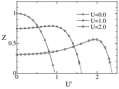
Figure 1: The quasi-particle weight $Z$ as a function of the inter-band Coulomb interaction $U^{\prime}$, obtained by the exact diagonalization $(N=6)$ within DMFT.

In the case $U=0$, $Z$ decreases monotonically with increasing $U^{\prime}$, and a metal-insulator transition occurs around $U^{\prime}_{c}\sim 0.9$. On the other hand, when $U\neq 0$, there appears nonmonotonic behavior in $Z$, namely, it once increases on the introduction of the interband Coulomb interaction, has the maximum value in the vicinity of $U^{\prime}\sim U$, and finally leads to a metal-insulator transition at a critical value of $U^{\prime}$. It is easily understood that the large value of $U^{\prime}$ suppresses hopping among sites, thereby causing a sharp decrease in the renormalization factor $Z$. However, it is somehow unexpected that the maximum structure appears around $U\sim U^{\prime}$, and furthermore is more enhanced for larger $U$ and $U^{\prime}$. We think that this is related to orbital fluctuations, which may stabilize a normal metallic state around $U\sim U^{\prime}$.

In order to observe the above behavior more clearly, we show the contour plot of the quasi-particle weight in Fig. 2.

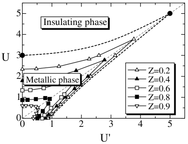
Figure 2: The contour plot of the quasi-particle weight $Z$ in the case $J=0$. The bold-dashed line represents the phase boundary of the metal-insulator transition, which is deduced by estimating the values of $U$ and $U^{\prime}$ that give $Z=0$. The solid circles are the transition points obtained by the linearized DMFT.

When $U^{\prime}=0$, the system is reduced to the single-band Hubbard model, where the intra-band Coulomb interaction $U$ induces the metal-insulator transition at $U_{c}$, which was estimated by the numerical renormalization group $(U_{c}=2.94)$,BullaNRG the exact diagonalization $(U_{c}=2.93)$,OnoED the linearized DMFT $(U_{c}=3)$.Bulla These values agree with the results in Fig. 2 well.

There are several remarkable features in this phase diagram. We first notice that the value of $Z$ is not so sensitive to $U^{\prime}$ for a given $U$ ($>U^{\prime}$), except for the region $U\sim U^{\prime}$. In particular, the phase boundary indicated by the dashed line in the upper side of the figure is almost flat for the small $U$ region. An important point to be noted is that when $U\sim U^{\prime}$ the metallic state is remarkably stable against a transition to the insulator, and persists up to fairly large Coulomb interactions. Moreover, it becomes immediately unstable, once the parameters are away from the line $U=U^{\prime}$. This tendency becomes more conspicuous in the regime of strong correlations. These remarkable properties about the metallic phase around the line $U=U^{\prime}$ are closely related to orbital fluctuations, as we will see momentarily in the following.

The second point is that there are two insulating phases corresponding to the regions $U>U^{\prime}$ and $U<U^{\prime}$, which are separated by the metallic phase for small $U,U^{\prime}$, but are continuously connected to each other via the region of large $U,U^{\prime}$. For example, let us observe phase transitions with $U=4.0$ being fixed. When $U^{\prime}=0.0$ with $U=4.0$, the system is in the insulating phase caused by the intra-band interaction $U$. Introducing the interband coupling $U^{\prime}$, a phase transition occurs to the metallic phase, and further increase in $U^{\prime}$ induces the second transition to another insulating phase, which is dominated by the inter-band interaction $U^{\prime}$. These two insulating phases should show different properties, though they can be adiabatically connected to each other in principle.

III.2 Critical properties around the phase boundary

To clarify the above characteristic properties around the metal-insulator transition, we exploit a linearized version of DMFT,Bulla which provides us with a transparent view of the phase transitions. In this scheme, we introduce a specific Anderson impurity model connected to only one host site, which corresponds to the model eq. (2) with $k=1$. This extreme simplification even provides sensible results as far as low-energy properties near the transition point are concerned. Namely, for low-energy excitations around the Fermi surface, the Green function for $f$-electrons may be approximated by a single pole as,

$$G_{\rm loc}(z) \sim \frac{w}{z},$$ (12)

where the residue $w$ corresponds to the quasi-particle weight. Recall that for $w=0$ the ground state belongs to an insulating phase, while for $w\neq 0$ to a metallic phase. We can thus determine the metal-insulator transition point from the condition $w=0$, as has been done before.

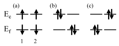
Figure 3: Three distinct singlet states in the Anderson model, which is hybridized with only one effective host site. The numbers 1, 2 specify the orbital indices.

By combining the self-consistent eqs. (4) and (7), we iterate the linearized DMFT. The self-consistent condition imposed on the hybridization now reads

$$V = \frac{\sqrt{w}}{2}.$$ (13)

For the single-band Hubbard model ($U^{\prime}=0$), the critical value $U_{c}=3$ was already estimated by the linearized DMFT.Bulla

In this simplified model, the metallic ground state is in the spin singlet state drawn in Fig. 3 (a) schematically. Although the introduction of the interband Coulomb interaction $U^{\prime}$ lowers the states (b) and (c) energetically, these states do not affect the ground-state properties up to a certain critical value of $U^{\prime}$. In fact, the relevant excitation gap is independent of $U^{\prime}$ in this approximation, and the residue of the Green function around $V=0$ is given as,

$$w = 36\left(\frac{V}{U}\right)^{2},$$ (14)

via a straightforward calculation. Then the self-consistent eq. (13) updates the hybridization via $(3/U)V\rightarrow V$ in each iteration process. Therefore, when $U>U_{c}(=3)$, the effective hybridization $V$ vanishes by the iteration, thereby stabilizing the insulating phase in this region. On the other hand, the hybridization is relevant for $U<U_{c}$ and thus the metallic phase is realized. Note that the critical value $U_{c}=3$ obtained here is the same as that for the single-band Hubbard model.Bulla We thus come to the conclusion that the inter-band Coulomb interaction has little effect on the metal-insulator transition, which is essentially described by the mechanism for the single-band Hubbard model, as far as the case of $U>U^{\prime}$ is concerned. This statement is indeed consistent with the numerical results shown in Fig. 2, namely, the phase boundary is rather insensitive to the change in $U^{\prime}$ for small $U^{\prime}$.

On the other hand, in the special case $U=U^{\prime}$, the nature of the transition is totally changed in this approximation. In this case, the ground state is formed by three degenerate states shown in Fig. 3, and not only spin but also orbital degrees of freedom play an important role. In fact, quantum fluctuations among these states decrease the effective mass, making the metallic phase more stable. The critical value $U_{c}=5$ estimated by the present scheme agrees with the numerical one in Fig. 2. Also this is consistent with the conclusion of quantum Monte Carlo simulations,Han which claims that the ground state in the single (double) orbital Hubbard model belongs to the insulating (metallic) phase in the case $U=U^{\prime}=4$.

The present analysis also gives a clear picture for two types of the metal-insulator transitions: the insulating phase in the upper region of in Fig. 2 corresponds to the state of Fig. 3(a), where the intra-atomic repulsion gives rise to the insulating phase, whereas the insulator in the lower region, corresponding to Fig. 3(b) and (c), is stabilized by the inter-band interaction. Around the critical point on the $U=U^{\prime}$ line, the metallic state sandwiched by these insulating phases is realized by the competition among almost degenerate singlet states (a), (b) and (c). In other words, the metallic state is stabilized by orbital fluctuations.

IV Effects of the Hund Coupling

IV.1 Isotropic case

We now discuss the effects of the exchange coupling $J$ between orbitals, which plays an important role in real materials such as manganites and ruthenates. By performing similar calculations, we obtain the contour plot of the quasi-particle weight $Z$ as shown in Fig. 4. We also plot the values of $Z$ as a function of $J$ in Fig. 5.

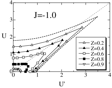
Figure 4: The contour plot of the quasi-particle weight $Z$ in the system with the ferromagnetic Hund coupling between the orbitals $J=-1.0$.

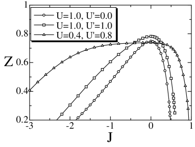
Figure 5: The quasi-particle weight $Z$ as a function of $J$.

The Hund coupling $J$ ($<0$) enhances spin correlations between the orbitals, thus renormalizing electrons near the Fermi surface. It is indeed seen in both figures that for $U>U^{\prime}$ the quasi-particle weight is decreased with the increase of $|J|$. On the other hand, the effect of the Hund coupling is less conspicuous in the region $U<U^{\prime}$. In the latter region, the inter-band Coulomb interaction dominates electron correlations in the ground state when $J=0$, which is schematically drawn as Fig. 3 (b) or (c). For these configurations the Hund coupling is irrelevant, which explains that the effect of $J$ is less important for $U<U^{\prime}$.

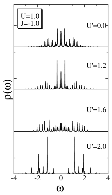
Figure 6: The density of states for $U^{\prime}=0.0,1.2,1.6$ and $2.0$ obtained by the exact diagonalization with $\delta=0.01$

To make the metal-insulator transition clear, we also calculate the density of states by means of the exact diagonalization. The results are shown in Fig. 6. When $U=1.0,J=-1.0$ and $U^{\prime}=0.0$, the system belongs to the metallic phase, as shown in Fig. 4. Introducing the interband coupling $U^{\prime}$, fluctuations between the orbitals are enhanced, which assist to stabilize the quasi-particle states up to $U^{\prime}\sim 1.2$. Further increase in $U^{\prime}$ favors the doubly occupied state in the same orbital. Therefore, the electron states around the Fermi surface are pushed away to higher energy regions, as seen in the case of $U^{\prime}=1.6$, and finally a quantum phase transition occurs from the metallic phase to the insulating phase. In the insulating phase for $U^{\prime}=2.0$, we can clearly see the charge gap in the density of states in Fig. 6.

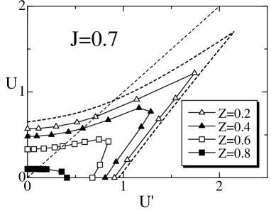
Figure 7: The contour plot of the quasi-particle weight $Z$ in the system with the antiferromagnetic exchange coupling between the orbitals $J=0.7$.

We also investigate the case of the antiferromagnetic exchange coupling $(J>0)$. The contour plot in the case $J=0.7$ is shown in Fig. 7. By comparing with the ferromagnetic case, it is seen that electrons are renormalized strongly, as shown in Fig. 5. This difference is explained by counting the number of effective degrees of freedom at each site in the presence of the exchange coupling. In the ferromagnetic case, the system has a tendency to form the $S=1$ state at each site, while in the antiferromagnetic case it favors the singlet state made of two orbitals. The resulting effective degrees of freedom give rise to the difference in the stability of the Fermi liquid state: the metallic state with the ferromagnetic coupling is more stable than the antiferromagnetic case. Note that the situation is similar to the stability of the metallic state due to orbital fluctuations around $U\sim U^{\prime}$ discussed in the previous section.

IV.2 Anisotropic case

We finally discuss the effects of anisotropy in the Hund coupling. For this purpose, we introduce the anisotropy parameter $\Delta$ as,

$$\left({\bf S}_{1}\cdot{\bf S}_{2}\right)_{\Delta} = \Delta\left(S_{1}^{x}S_{2}^{x}+S_{1}^{y}S_{2}^{y}\right)+S_{1}^{z}S_{2}^{z},$$ (15)

where $\Delta=0$ corresponds to the Ising-type anisotropy, while $\Delta=1$ the isotropic case. In Fig. 8, we show the quasi-particle weight $Z$ for $U=1.0$ and $J=-1.0$.

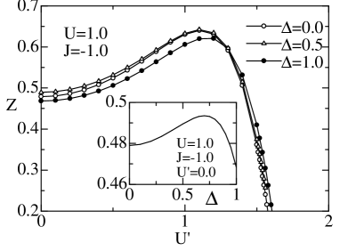
Figure 8: The quasi-particle weight $Z$ for the case with anisotropic exchange coupling: $U=1.0$ and $J=-1.0$. Inset shows the quasi-particle weight as a function of the anisotropy parameter $\Delta$.

In the ferromagnetic case, the quasi-particle weight $Z$ is little affected by anisotropy although somewhat nonmonotonic dependence is found as a function of $\Delta$ as shown in the inset. On the contrary, the anisotropy has a noticeable effect for the antiferromagnetic case with small $U^{\prime}$, as seen from Fig. 9, where the anisotropy decreases the weight $w$ monotonically with the increase of $\Delta$. This difference arises from the fact that the $x-y$ components of the exchange coupling bring about quantum fluctuations more prominently in the antiferromagnetic case than in the ferromagnetic case, giving rise to the sizable effect on the antiferromagnetic case in the small $U^{\prime}$ region.

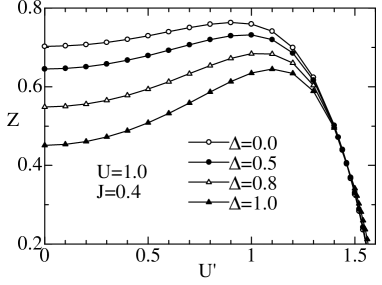
Figure 9: The quasi-particle weight $Z$ as a function of $U^{\prime}$ in the case $U=1.0$.

V Summary

We have investigated the stability of a metallic phase in the two-orbital Hubbard model at half-filling by means of dynamical mean-field theory with particular emphasis on the role played by orbital degrees of freedom. By combining the exact diagonalization method with DMFT, we have discussed how the interplay among the intra-band and inter-band Coulomb interaction together with the Hund coupling affects the metal-insulator transition. In particular, it has been found that the metallic state is remarkably stable, even up to $U\sim 5.0$ if the intra and inter-band Coulomb interactions are nearly equal. Also, slight deviation from this condition immediately drives the system to the insulating phase. We have pointed out that orbital fluctuations play a particular role to realize the metallic state around $U\sim U^{\prime}\sim 5.0$. The effect of the exchange coupling has been also discussed. It has been clarified that the effective degrees of freedom at each site play an important role again in stabilizing the metallic state.

We have focused on nonmagnetic phases of the model in this paper. Possible instabilities toward other ordered states such as the magnetic order, the superconductivity, etc., are to be studied. In particular, the ferromagnetic instability is interesting in connection with ferromagnetism realized in manganite compounds. These problems are now under consideration.

VI Acknowledgments

We would like to thank M. Suminokura for useful discussions. This work was partly supported by a Grant-in-Aid from the Ministry of Education, Science, Sports and Culture of Japan. A part of computations was done at the Supercomputer Center at the Institute for Solid State Physics, University of Tokyo and Yukawa Institute Computer Facility.

References

- (1) Y. Tokura, A. Urushibara, Y. Moritomo, T. Arima, A. Asamitsu, G. Kido and N. Furukawa, J. Phys. Soc. Jpn. 63, 3931 (1994).
- (2) Y. Maeno, H. Hashimoto, K. Toshida, S. Nishizaki, T. Fujita, J. G. Bednorz, F. Lichtenberg, Nature, 372, 532 (1994).
- (3) M. Imada, A. Fujimori and Y. Tokura, Rev. Mod. Phys. 70, 1039 (1998); Y. Tokura and N. Nagaosa, Science 288, 462 (2000).
- (4) T. M. Rice and M. Sigrist, J. Phys. Condens. Matt. 7, L643 (1995).
- (5) S. Kondo, D. C. Johnston, C. A. Swenson, F. Borsa, A. V. Mahajan, L. L. Miller, T. Gu, A. I. Goldman, M. B. Maple, D. A. Gajewski, E. J. Freeman, N. R. Dilley, R. P. Dickey, J. Merrin, K. Kojima, G. M. Luke, Y. J. Uemura, O. Chmaissem and J. D. Jorgensen, Phys. Rev. Lett. 78, 3729 (1997).
- (6) H. Kaps, N. Büttgen, W. Trinkl, A. Loidl, M. Klemm and S. Horn, J. Phys. Condense. Matter, 13, 8497 (2001).
- (7) M. Isoda and S. Mori, J. Phys. Soc. Jpn. 69, 1509 (2000).
- (8) S. Fujimoto, Phys. Rev. B 64, 085102 (2001).
- (9) H. Tsunetsugu, preprint.
- (10) Y. Yamashita and K. Ueda, preprint.
- (11) H. Hasegawa, J. Phys. Soc. Jpn. 66, 1391 (1997).
- (12) S. Ishihara, M. Yamanaka and N. Nagaosa, Phys. Rev. B 56, 686 (1997); R. Maezono, S. Ishihara and N. Nagaosa, Phys. Rev. B 58, 11583 (1998).
- (13) R. Frésard and G. Kotliar, Phys. Rev. B 56,12909 (1997).
- (14) A. Klejnberg and J. Spalek, Phys. Rev. B 57, 12041 (1998).
- (15) J. Bünemann, W. Weber and F. Gebhard, Phys. Rev. B 57, 6896 (1998).
- (16) Y. Motome and M. Imada, J. Phys. Soc. Jpn. 67, 3199 (1998).
- (17) G. Khaliullin and S. Maekawa, Phys. Rev. Lett. 85, 3950 (2000).
- (18) T. Takimoto, Phys. Rev. B 62, R14641 (2000).
- (19) T. Momoi and K. Kubo, Phys. Rev. B 58, R567 (1998).
- (20) M. J. Rozenberg, Phys. Rev. B 55, R4855 (1997).
- (21) K. Held and D. Vollhardt, Eur. Phys. J. B 5, 473 (1998).
- (22) J. E. Han, M. Jarrell and D. L. Cox, Phys. Rev. B 58, R4199 (1998).
- (23) V. S. Oudovenko and G. Kotliar, Phys. Rev. B 65, 075102 (2002).
- (24) G. Kotliar and H. Kajueter, Phys. Rev. B 54, R14221 (1996).
- (25) W. Metzner and D. Vollhardt, Phys. Rev. Lett. 62, 324 (1989).
- (26) E. Müller-Hartmann, Z. Phys. B 74, 507 (1989).
- (27) A. Georges, G. Kotliar, W. Krauth and M. J. Rozenberg, Rev. Mod. Phys. 68, 13 (1996).
- (28) T. Pruschke, M. Jarrell, and J. K. Freericks, Adv. Phys. 42, 187 (1995).
- (29) M. Caffarel and W. Krauth, Phys. Rev. Lett. 72, 1545 (1994).
- (30) Th. Pruschke, D. L. Cox and M. Jarrell: Phys. Rev. B 47 (1993) 3553.
- (31) O. Sakai and Y. Kuramoto, Solid State Comm. 89, 307 (1994).
- (32) R. Chitra and G. Kotliar, Phys. Rev. Lett. 83, 2386 (1999).
- (33) J. Joo and V. Oudovenko, Phys. Rev. B 64, 193102 (2001).
- (34) M. S. Laad, L. Craco and E. Müller-Hartmann, Phys. Rev. B 64, 195114 (2001).
- (35) R. Bulla, Phys. Rev. Lett. 83, 136 (1999).
- (36) A. Georges, G. Kotliar and W. Krauth, Z. Phys. B 92, 313 (1993).
- (37) Th. Maier, M. B. Zölfl, Th. Pruschke and J. Keller, Eur. Phys. J. B 7, 377 (1999).
- (38) Y. Imai and N. Kawakami, J. Phys. Soc. Jpn. 70, 2365 (2001).
- (39) Y. Ono, R. Bulla and A. C. Hewson, Eur. Phys. J. B 19, 375 (2001); Y. Ohashi and Y. Ono, J. Phys. Soc. Jpn. 70, 2989 (2001).
- (40) M. Jarrell, H. Akhlaghpour and T. Pruschke, Phys. Rev. Lett. 70, 1670 (1993).
- (41) T. Mutou and D. Hirashima, J. Phys. Soc. Jpn. 63, 4475 (1994);
- (42) T. Saso and M. Itoh, Phys. Rev. B 53, 6877 (1996);
- (43) R. Bulla and M. Potthoff, Eur. Phys. J. B 13, 257 (2000).
- (44) R. Haydock, V. Heine and M. J. Kelly, J. Phys. C 8, 2591 (1975).