Abstract

We have performed a number of experiments with a Bose-Einstein condensate (BEC) in a one dimensional optical lattice. Making use of the small momentum spread of a BEC and standard atom optics techniques a high level of coherent control over an artificial solid state system is demonstrated. We are able to load the BEC into the lattice ground state with a very high efficiency by adiabatically turning on the optical lattice. We coherently transfer population between lattice states and observe their evolution. Methods are developed and used to perform band spectroscopy. We use these techniques to build a BEC accelerator and a novel, coherent, large-momentum-transfer beamsplitter.

A Bose-Einstein Condensate in an optical lattice

J Hecker Denschlag, J E Simsarian, H Häffner†, C M^cKenzie, A Browaeys, D Cho, K Helmerson, S L Rolston, and W D Phillips

An optical lattice is a practically perfect periodic potential for atoms, produced by the interference of two or more laser beams. A Bose-Einstein condensate (BEC) [1, 2] is the ultimate coherent atom source, a collection of atoms, all in the same state, with an extremely narrow momentum spread. Combining a BEC with an optical lattice provides an opportunity for exploring a quantum system analogous to electrons in a solid state crystal but with unprecedented control over both the lattice and the particles.

Periodic optical potentials have been widely used in atomic physics (For reviews see [3, 4, 5]). Recent experiments and theory have studied BECs in optical lattices [6, 7, 8, 9, 10, 11, 12, 13, 14, 15, 16, 17, 18][19, 20, 21, 22, 23, 24, 25]. Here we present a series of new experiments in which we precisely manipulate the BEC/lattice system and interpret the results in terms of a single-particle band structure theory.

We describe 1D lattice experiments with a sodium BEC in a regime where interactions between atoms are negligible. This paper is organised as follows: we begin with a description of the experimental arrangement (Sec. 1) and a brief summary of band theory (Sec. 2). We explore diabatic and adiabatic loading of a BEC into a lattice in Sec. 3. Using momentum state analysis we measure coherent superpositions between bands and determine that we can adiabatically load more than 99% of the atoms into a well-defined Bloch state. In Sec. 4 we manipulate the lattice potential to transfer population between Bloch states, mapping the band structure of the lattice eigenstates. We follow the work of [26, 27, 28] in Sec. 5 in the deep lattice regime to develop a BEC accelerator which imparts many photon recoils of momentum to the atoms while preserving the coherence of the condensate. With a little modification we turn the accelerator into a large momentum transfer beamsplitter, which is described in Sec. 6.

1 Experimental setup

We perform our experiments with a condensate of $3(1)\times 10^{6}$ sodium atoms  in the $3S_{1/2}$, $F=1$, $m_{F}=-1$ state. The sample has no discernible thermal component. The condensate is prepared as described in [8] and is held in a magnetic time-orbiting potential (TOP) [29, 8] trap with trapping frequencies $\omega_{x}=\sqrt{2}\omega_{y}=2\omega_{z}=2\pi\times$27 Hz. Assuming a scattering length of $a=2.8$ nm, the calculated Thomas-Fermi diameters [30] are 47, 66, and 94 $\mu$m, respectively. The size and density of the BEC are such that the condensate populates on the order of a hundred lattice wells and interactions between atoms can be ignored on the time-scale of our experiments.

After production of the condensate the optical lattice is turned on. It consists of two counter-propagating laser beams along the $x$-direction whose frequencies and amplitudes can be controlled independently by acousto-optic modulators (AOMs). The lattice beams are detuned about $60$ GHz to the blue of the atomic resonance (the sodium D₂ line: $\lambda=2\pi/k=589$ nm) so that the spontaneous emission rate ($\sim 100$ s^-1) is negligible on the time scale of our experiments. The polarization is linear and parallel to the rotation axis of the TOP trap bias field (the $y$ axis). The condensate is located in the focus of the beams, which have a $1/e^{2}$ diameter of about 600 $\mu$m. The maximum power used in each beam is about 4 mW.

The two counter-propagating laser beams form a standing wave, which acts on the atoms via the light-shift [31] to produce a sinusoidal potential:

$$V(x,t)=\frac{V_{0}}{2}\left(1+\cos(2kx+\delta t)\right).$$ (1)

Here $\delta$ is the frequency difference between the two laser beams. This detuning gives the standing wave a velocity of $v=\delta/2k$. A frequency difference of $\delta/(2\pi)=100$ kHz corresponds to a lattice velocity of $3$ cm$\cdot$s^-1 (one photon recoil).

We use time-of-flight analysis [7] to examine the momentum distributions that result from our experiments. At the conclusion of the experiment we turn the magnetic trap off abruptly and the lattice is removed. The details of the turn-off of the lattice depend on the experiment and will be described later. Two milliseconds of free-flight allows the momentum components (which are discrete and separated by 2$\hbar k$ due to the periodicity of the lattice) to spatially separate. We then measure the number of atoms in each momentum state by absorption imaging with a CCD camera.

We adjusted the laser power and detuning such that the height of the lattice potential $V_{0}$ (measured as described in Sec. 3.1) was typically 14 photon recoil energies, $E_{R}=\hbar^{2}k^{2}/2M$. $M$ is the atomic mass of sodium; $E_{R}/h=25$ kHz. The total power was constant to within $10\%$.

2 Band structure in an optical lattice

Band structure theory is derived assuming an infinite periodic potential. Our lattice period ($\approx 0.3\ \mu$m) is small compared to the Thomas-Fermi diameter (47 $\mu$m) of the condensate in the lattice direction. Hence, the atomic wavefunction covers more than a hundred lattice sites and the system can be considered practically infinite. The corresponding momentum spread of the BEC is very small ($\sim 0.01\hbar k$), so we treat the BEC as a plane wave. Also, atom-atom interactions are negligible: the time-scale associated with the peak chemical potential, $\hbar/\mu=1/(2\pi\times 800\;\mathrm{Hz})=280$ $\mu$s, is longer than the 20 $\mu$s time scale of our typical experiments. Thus, a single-particle picture is valid.

The periodicity of the lattice leads to a band structure of the energy spectrum of the atom-lattice system. The eigenenergies $E_{n,q}$ and eigenstates $|n,q\rangle$ (Bloch states) of the system in the rest frame of the lattice are labeled by the quasimomentum $q$ and the band index $n$. The spatial periodicity of the eigenfunctions results in a momentum spectrum composed of peaks separated by the momentum corresponding to the reciprocal lattice vector, $2\hbar k$. The Bloch states $|n,q\rangle$ can thus be expanded in the discrete plane wave basis $|\phi_{p}\rangle$ with momenta $p=q+2m\hbar k$ :

$$|n,q\rangle=\sum_{m=-\infty}^{\infty}a_{n,q}(m)|\phi_{q+2m\hbar k}\rangle\ .$$ (2)

In order to calculate the coefficients $a_{n,q}(m)$ and the eigenenergies $E_{n,q}$ we solve the equation $\hat{H}|n,q\rangle=E_{n,q}|n,q\rangle$ where the Hamiltonian is $\hat{H}=\hat{P}^{2}/2M+(V_{0}/2)\cos(2kx)$.

Figure 1 shows the eigenenergies versus quasimomentum for the first five bands ($n=0$ through 4) from $q=-\hbar k$ to $\hbar k$ (the first Brillouin zone) for $V_{0}=14E_{R}$. Even in this relatively shallow potential the $n=0$ band is quite flat indicating that the tunneling rate is low.

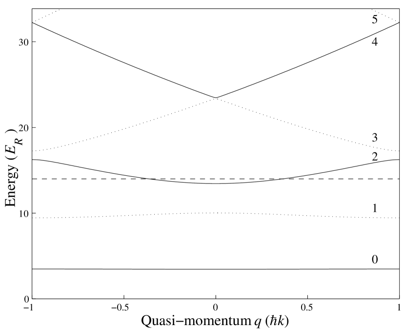
Figure 1: The first five bands (even bands are solid, odd bands are dotted) of a 14$E_{R}$ deep, 1D, sinusoidal lattice across the first Brillouin zone. The dashed horizontal line indicates the top of the lattice.

Figure 2 shows the plane wave decomposition, $|a_{n,q}(m)|^{2}$, of the Bloch eigenstates for the bands $n=0$, 1, 2, and 3 at $q$ = 0 and $V_{0}=14E_{R}$. For example, the lattice ground state $|n=0,q=0\rangle$ consists mainly (65 %) of a 0 momentum component and two smaller $\pm 2\hbar k$ momentum components (17 % each).

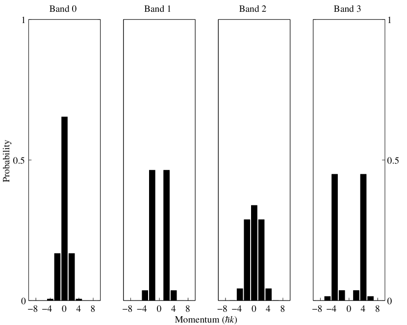
Figure 2: The lattice eigenstates can be expressed as a superposition of plane waves with fractional population $|a_{n,q}(m)|^{2}$. Shown is the plane wave decomposition of the lattice eigenstates for the four lowest bands for $q=0$ and lattice height $V_{0}$ = 14$E_{R}$.

The spatial wave function of a Bloch eigenstate in the lattice frame, $\psi_{n,q}(x)=\langle x|n,q\rangle$, obeys Bloch’s theorem:

$$\psi_{n,q}(x+\lambda/2)=e^{iq\lambda/2\hbar}\ \psi_{n,q}(x)\ .$$ (3)

The quasimomentum characterizes the phase difference between neighbouring lattice sites.

Optical lattices have the advantage that we can easily change their depth and velocity. In the absence of an external force (or equivalently an acceleration of the lattice), the quasimomentum is conserved (even if the depth changes) as long as the lattice periodicity is kept constant. (Recall that quasimomentum is only defined in the rest frame of the lattice.) For an optical lattice this is obvious since the only mechanism for changing momentum in the absence of spontaneous emission is redistribution of photons from one lattice beam to the other. Hence the momentum can only change by multiples of 2$\hbar k$, which does not change the quasimomentum (see equation (3)).

3 Loading the BEC into the lattice

We now discuss methods for loading the BEC into the lattice with a selected quasimomentum $q$. We investigate two regimes: the sudden turn-on and the adiabatic turn-on.

A BEC makes it easy to load a lattice state with a well-defined quasimomentum. Its small momentum spread (of much less than $\hbar k$) results in an similar spread of the quasimomentum $q$. For a condensate stationary relative to the lattice, the phase of the BEC is uniform across the lattice, hence $q=0$. By contrast, when the condensate is moving with velocity $v$ relative to the lattice, there is a linear phase gradient across the condensate and $q=-Mv$.

3.1 Sudden loading of the lattice

A BEC, taken to be a plane wave ($|\Psi(t=0)\rangle=|\phi_{q}\rangle$), suddenly loaded into a lattice can be described as a superposition of Bloch states $|n,q\rangle$ :

$$|\Psi(t=0)\rangle=\sum_{n=0}^{\infty}|n,q\rangle\langle n,q|\phi_{q}\rangle\ .$$ (4)

From equation (2), $\langle n,q|\phi_{q}\rangle=a^{*}_{n,q}(0)$. Therefore while the BEC wavepacket is held in the lattice it evolves in time according to

$$|\Psi(t)\rangle=\sum_{n=0}^{\infty}a_{n,q}^{*}(0)\,\exp\left\{-iE_{n}(q)t/\hbar\right\}|n,q\rangle\;.$$ (5)

We suddenly switch the lattice off after a time $\tau$. If we project the lattice state onto the plane wave (measurement) basis, we obtain the coefficients $b_{q}(m)$ of each $|\phi_{q+2m\hbar k}\rangle$ in the lattice frame:

$$b_{q}(m)=\sum_{n=0}^{\infty}a^{*}_{n,q}(0)\ a_{n,q}(m)\ \exp\left(-i\ \frac{E_{n}(q)}{\hbar}\ \tau\right).$$ (6)

The interference of the exponential factors produces oscillations in the populations of the plane wave components as a function of $\tau$.

We observe these oscillations as follows: after producing the BEC we quickly (within 0.5 $\mu$s) turn on the lattice beams and leave them on for a variable length of time $\tau$. We then shut the lattice off abruptly (again within 0.5 $\mu$s) and measure, after a time of free-flight, the relative populations of the momentum components .

Figure 3 shows the time evolution of a BEC held in the stationary lattice ($q=0$). The populations vary almost purely sinusoidally, because only bands 0 and 2 are significantly populated. Band 1 and all odd bands are not populated because the symmetry of those eigenstates are antisymmetric while the initial BEC wavefunction is essentially uniform (effectively symmetric) across a single well. The observed oscillation period of 250 kHz is the energy gap between band 0 and 2 for a 14$E_{R}$ deep lattice. We use this frequency to calibrate our lattice depth.

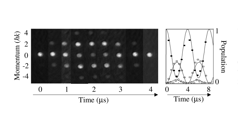
Figure 3: Coherent oscillations of the momentum decomposition of a BEC after suddenly switching on the lattice ($q$ = 0, $V_{0}=14E_{R}$). On the left are time of flight images showing the plane wave decomposition of the lattice state evolving as a function of time held in the lattice. The momentum components have been allowed to spatially separate. Only a single 4 $\mu$s cycle is shown. The right hand shows the populations of the 0, +2 and +4$\hbar k$ momentum components (respectively: the filled squares, open squares and circles) over two cycles. The lines are a theoretical calculation of the populations in each component.

We can also load the condensate into a lattice moving with a constant velocity relative to the BEC. In the rest frame of the lattice this corresponds to loading a specific non-zero $q$. Figure 4 shows the results of an experiment, similar to that shown in figure 3, for $q=1\hbar k$. The oscillations are not sinusoidal because more than two bands have significant population. Odd bands 1 and 3 are now populated in addition to bands 0 and 2 because the selection rules discussed above are not valid for $q\neq 0$. The resulting beating signal consists of a superposition of sinusoids of different frequencies (see equation (6)) corresponding to the energy differences between pairs of bands. Our observations can be reproduced by the simple 1D band model, as shown in the right hand side of figure 4. We have also performed the sudden loading experiment for other $q$ between 0 and 1$\hbar k$ and the results agree well with the model.

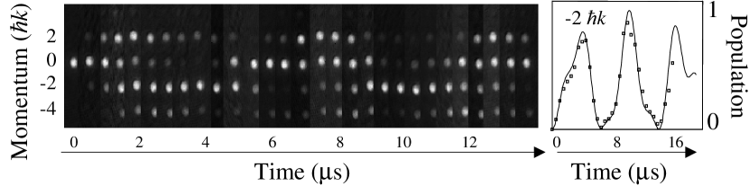
Figure 4: Coherent oscillations of a BEC after suddenly switching on the lattice for $q$ = 1$\hbar k$. This is the same as the experiment shown in figure 3, only the quasimomentum has been changed. This time the oscillations are not sinusoidal. The right hand side plot shows the evolution of the $-2\hbar k$ component. The standard 1D band model describes the data well, as shown by the full line.

We have measured the decay time of the beat signal by extending the lattice interaction time $\tau$. Figure 5 shows the decaying oscillations of the $0\hbar k$ component for $q=0$. We fit this data with an exponentially decaying sinusoid with a decay constant of $17\ \mu$s. Notice that the data scatters widely at long times. This implies that the decay is due to two mechanisms: the inhomogeneity ($\approx 10\%$) of our lattice beams over the condensate and laser power fluctuations from shot to shot (also about 10%).

Figure 5: As the lattice is held on for longer times the amplitude of the oscillation signal decreases. This is due to two factors, inhomogeneity of the lattice beams and shot-to-shot variation in the lattice strength. Both of these effects lower the oscillation amplitude by averaging several oscillations which are slightly out of phase with each other. The inhomogeneity of the beams affects each data point and this decay is the decay of the envelope of the data points (this is indicated by the dashed lines which have been drawn to guide the eye). The shot-to-shot intensity fluctuations only have an effect when the data is averaged or a fit is made. This can be seen in the solid line which is a fit of a decaying sinusoid to the data points: the decay of the fit is faster than the decay of the envelope. Both these effects have to be taken into account when analysing the data.

3.2 Adiabatic loading of the lattice

In contrast to the preceding section, where we populated several bands by suddenly turning on the lattice, here we transfer the BEC into a single Bloch state $|n,q\rangle$. To achieve this we ramp up the lattice intensity adiabatically, i.e., such that [32]

$$\left|\left\langle i,q\left|\frac{\partial H}{\partial t}\right|0,q\right\rangle\right|\ll\Delta E^{2}(q,t)/\hbar.$$ (7)

where $\Delta E$ is the energy difference between the ground state and the first excitable state $|i\rangle$. The left hand side is always less than $\mathrm{d}V_{0}/\mathrm{d}t$. Therefore the condition in (7) can be satisfied at $q=0$ by choosing $\mathrm{d}V_{0}/\mathrm{d}t<<16E_{R}^{2}/\hbar$ since $\Delta E\geq 4E_{R}$ for any $V_{0}$ (see figure 6). It becomes harder to maintain adiabaticity as $q$ approaches the Brillouin zone boundary since there $\Delta E=0$ when $V_{0}=0$. The manifestation of the non-adiabaticity is Bragg scattering. For our experiments, at $q=0$ with a final lattice depth of 14$E_{R}$, an adiabatic ramp must be significantly longer than 5 $\mu$s.

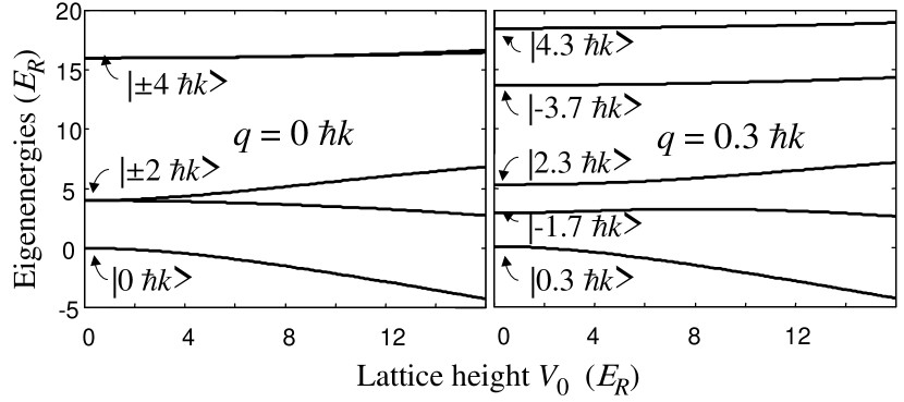
Figure 6: The energy eigenspectrum for two values of the quasimomentum, $q=0$ (left) and $q=0.3\hbar k$ (right), as a function of the lattice height $V_{0}$. At $V_{0}=0$ the lattice eigenenergies are the free particle kinetic energies, $p^{2}/2M$ and the eigenstates are the plane waves with momentum $p=2m\hbar k+q$ (in the lattice frame).

Note that this adiabaticity criterion takes into account only the single particle motion. We are very non-adiabatic with respect to the time scale associated with atom-atom interaction energies. Recent experiments, which observe number squeezing [17] and the Mott transition [18], depend on being adiabatic on this longer time scale.

If we can adiabatically ramp up the lattice intensity then we should also be able to adiabatically ramp down the intensity and return to the original BEC. This suggests an obvious test for adiabaticity where we ramp the intensity up and then down over equal time intervals. The degree of adiabaticity can be determined by measuring the number of atoms excited into momentum components other than 0 $\hbar k$. The results of this experiment are shown in figure 7.

This method has two limitations: Firstly, the sensitivity is limited to the fraction of atoms that can be reliably detected, a few percent in our case. Secondly, interference between populated bands (as seen in the previous section) can lead to all the population being in 0 $\hbar k$ even though the process is far from adiabatic. Because of this, the signal oscillates and the adiabaticity of a single ramp time can only be determined by interpolating the envelope of the curve.

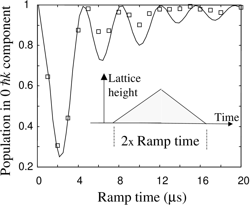
Figure 7: Testing the adiabaticity of a linear intensity ramp with a double ramp. Perfect adiabaticity would leave all the atoms in the 0 $\hbar k$ state. If the ramp is not fully adiabatic other momenta are populated. The observed oscillations in the 0 $\hbar k$ component are due to interference effects similar to the ones described in section 3. The full line is a theoretical model obtained through direct integration of the Hamiltonian. It has been rescaled by about 10% in the time direction to match the data.

In order to directly measure the adiabaticity, i.e. the transfer efficiency into the lattice ground state, we perform experiments similar to those described in the previous section. Starting from a condensate at rest we ramp up the intensity of a stationary lattice. We hold the BEC in the lattice for a time $\tau$, typically between 0 to 10 $\mu$s, before suddenly switching off the light. We then study the oscillations in the plane wave decomposition of the lattice wavefunction as a function of $\tau$. Figure 8 shows an example of such oscillations for the $0\hbar k$ component at $q=0$ after a ramp time of 20 $\mu$s. This beating signal has a very small amplitude compared to the beating signal of figure 3 for a lattice that was abruptly switched on. This indicates that most of the population is in band 0. If we had populated only the ground state, there would have been no beating at all. If we ignore the small oscillations, the measured momentum decomposition (60 % $0\hbar k$, 20 % $+2\hbar k$, 20 % $-2\hbar k$) is close to the theoretical decomposition of the lattice ground state (Sec. 2).

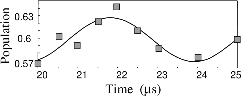
Figure 8: Residual oscillations in the plane wave decomposition of a lattice state loaded by slowly ramping up the lattice over $20\mu$s. The beating is greatly reduced when we raise the lattice in this manner because the condensate has been loaded almost entirely into the lattice ground state. This data has been averaged, but not corrected for loss of amplitude due to inhomogeneity in the lattice beams or shot-to-shot variations in the lattice height.

From the amplitude of the oscillations we can infer the population in the lattice ground state. To do this, we assume that only band 0 and 2 are populated (since bands 1 and 3 cannot be excited at $q=0$). Let $p$ be the fraction of the population in band 0 after loading into the lattice. Then the population in band 2 is $1-p$. For a lattice with a height of $14E_{R}$ band 0 has a calculated $0\hbar k$ momentum component of 65 % whereas band 2 has one of 34 % (see figure 2). The fraction of population in the $0\hbar k$ momentum component after evolving for a time $\tau$ is

$$P(\tau)=\left|\sqrt{0.65p}+e^{i(\omega\tau+\theta)}\sqrt{0.34(1-p)}\right|^{2}\ \,$$ (8)

where $\omega$ is the frequency difference between bands 0 and 2 and $\theta$ is a phase that is dependent on the details of the ramp. The amplitude of the beating is

$$\Delta P=2\sqrt{0.65p\times 0.34(1-p)}.$$ (9)

Equation (9) does not take into account the decay of the beating amplitude due to dephasing. Before calculating $p$ from the experimentally measured value for $\Delta P$, we must first correct for the dephasing. We cannot directly use the decay rate obtained from figure 5 since, in this case, we use an intensity ramp rather than a constant intensity. To find the correct decay rate a simulation of the sudden turn on was performed with the effects of shot-to-shot noise and beam inhomogeneity included. The simulation was a direct solution of Schrödinger’s equation with no mean-field effects. The parameters of the dephasing effects were then adjusted to match the observed decay and were then applied to a similar simulation which included the intensity ramp.

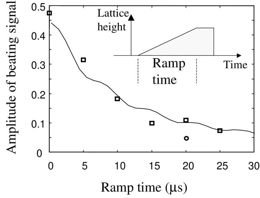
Figure 9: The decrease of the beating signal with increasing ramp time for a final lattice height of 14$E_{R}$. The data points are corrected to account for loss of coherence. The full line is from a band-theory calculation for a lattice with $V_{0}=14E_{R}$. The insert sketches how the lattice height is ramped during the experiment. The open circle corresponds to the data in figure 8.

Figure 9 shows how the oscillation amplitude decreases as a function of the lattice ramp time. The data are corrected for decay as described above. The largest correction is a factor of 1.8 increase in the oscillation amplitude. The data agree well with a calculation (full line) where the single-particle Hamiltonian corresponding to loading a $V_{0}=14E_{R}$ lattice is numerically solved. The lowest amplitude shown in figure 9 (the open circle, this data is shown in figure 8) corresponds to a ramp time of 20 $\mu$s and a groundstate population of 99.7(1)% (the uncorrected result is 99.9%).

Finally we point out that a linear ramp is not the most efficient way to populate the ground state. Numerical simulations show that our actual ramp (smoothed by the AOM response) is more adiabatic than a linear ramp. These simulations agree well with our observed adiabaticity. Other ramp shapes could be made even more adiabatic. Since the band gap increases with the lattice intensity, the ramp can be accelerated as the intensity increases.

As an alternative we find that we can dramatically improve the loading of the ground state by using interference effects. The single linear ramp can for example be broken up into two linear ramps with different slopes. Both ramps coherently drive population between the ground and excited states. The second ramp can then be used to almost entirely cancel the effect of the first ramp. Details of these studies will be subject of future work.

4 Coherent Transfer between Lattice Bands and Band-spectroscopy

Starting from a condensate adiabatically loaded (20 $\mu$s ramp) into the ground state of the lattice, we will now study coherent population transfer to higher bands.

4.1 Transfer between bands 0 and 1

To transfer population from band 0 to 1 at $q=0$ (see figure 10) we modulate the phase of one of the lattice beams and thus the position of the wells, i.e. shaking the lattice. The modulation is performed using an AOM and has an amplitude of $\approx\pi/6$. We apply the modulation for four cycles over approximately 30 $\mu$s.

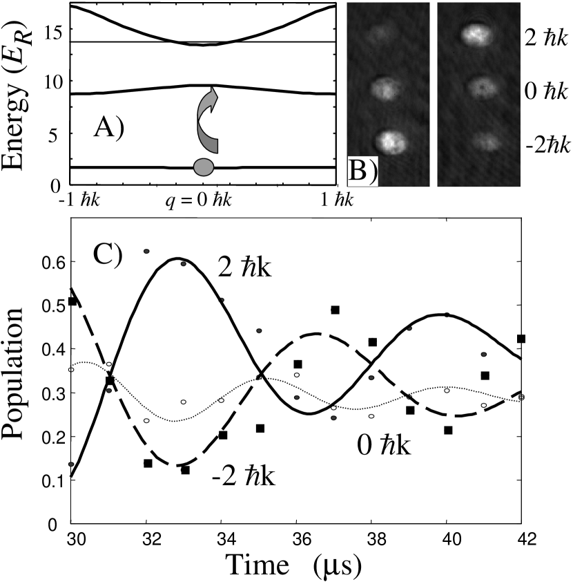
Figure 10: Starting from the lattice ground state ($q=0$, $n$ = 0) population can be coherently transferred to the band 1 (at $q=0$) by shaking the lattice for 30 $\mu$s. This is illustrated in A. In B and C the oscillations in the plane wave decomposition of the lattice state are shown after transferring some population to band 1. Oscillations are strongest between the $\pm 2\hbar k$ components. Fitting exponentially decaying sinusoids (C) to the oscillating momentum components yields an oscillation frequency of 140 kHz for the $\pm 2\hbar k$ components.

Shaking the lattice is an odd-parity excitation and therefore efficiently couples bands of opposite parity, such as bands 0 and 1. The phase modulation can also be viewed as putting sidebands on the lattice beam. In this picture the transition between bands is a Raman transition and the ability to make odd parity excitations is related to the phase difference of $\pi$ between the sidebands.

A convenient way to analyze the population of excited bands is to adiabatically ramp down the lattice after the shaking. Population in band 1 at $q=0$ is all transferred, after the ramp-down, into the $\pm 2\hbar k$ components. The frequency of the 0 to 1 transition can then be found by maximising the population in these momentum components.

Once the resonance is found we can examine the population transfer via interference experiments. If we switch off the lattice suddenly we observe oscillations as a function of the holding time (see figure 10 B and C). Since bands 0 and 1 have opposite parity the oscillations will tend to be between momentum components with opposite momenta (in contrast to the beating of bands 0 and 2 illustrated in figure 3). Fitting an exponentially decaying sinusoid to the oscillating momentum components yields an oscillation frequency of 140 kHz for the $\pm 2\hbar k$ components consistent with the calculated frequency of 147 kHz for the 11$E_{R}$ lattice used for this experiment. The oscillations show that we have coherently populated band 1. The small oscillation of the 0 $\hbar k$ momentum peak is due to population in band 2 (the oscillation frequency corresponds to the energy gap between bands 0 and 2) that has been excited by second-order processes.

4.2 Transfer between bands 0 and 2

We can transfer population between bands 0 and 2, without exciting band 1, by amplitude-modulation of the lattice, an even-parity excitation. This can be viewed as a Raman process as well; in this case the sidebands are in phase.

Although band 1 is relatively flat, band 2 has significant curvature (see Figs. 1 and 11 A) which can be examined by varying $q$ and measuring the resonance frequency. The resonance is found by varying the modulation frequency to maximise the loss from band 0.

Figure 11: The scheme for transferring population into band 2 at arbitrary $q$. We start from the ground state at a quasimomentum of 0. We then accelerate the lattice to change the quasimomentum from 0 to the desired value of $q$. Population is transferred into band 2 by modulating the lattice height over a 20 to 30 $\mu$s period. In order to measure the population in the upper band the acceleration is reversed to bring the quasimomentum back to 0 and the lattice is adiabatically released to map the bands into individual momentum components.

To produce a non-zero $q$ within the first Brillouin zone we start from an adiabatically loaded lattice ground state ($q=0$) and then suddenly apply a constant acceleration $a=300$ m$\cdot$s^-2 to the lattice. For $|Ma\langle 1,0|x|0,0\rangle|\ll\Delta E$ (corresponding to $a<3.9\times 10^{4}\;m\cdot s^{-2}$ in our case) this sudden change does not significantly excite higher bands. In the lattice frame the inertial force changes $q$ according to $\mathrm{d}q/\mathrm{d}t=Ma$. We adjust the duration of the acceleration to obtain the desired $q$. (We could have adiabatically loaded the condensate directly into a moving lattice to produce a non-zero $q$, but achieving adiabaticity is difficult near $q=1\hbar k$.)

We suddenly stop accelerating, holding $q$ constant. The lattice height is then modulated by 15% (controlled with an AOM) for 6 to 7 oscillations. Using this relatively short and strong agitation to transfer the population broadens the transition and makes it easier to find the resonance line. In order to measure how much population has been transferred to band 2, the lattice is decelerated to zero velocity ($q=0$) and then adiabatically ramped down to map the lattice bands into plane waves (see figure 6). Figure 12 shows the resonance curve for $q=1\hbar k$. The resonance frequency at about 320 kHz equals the expected band gap between band 0 and 2 at $q=1\hbar k$. The width of the excitation is determined by the bandwidth of the excitation ($\approx 37$ kHz). In the insert we plot the measured resonance frequencies for the quasimomenta $q$ = 0, 0.25, 0.5, 0.75 and 1$\hbar k$ together with the calculated band structure for $V_{0}=14E_{R}$. The data agrees well with the band model.

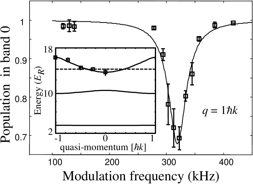
Figure 12: Experimental data showing population transfer from band 0 to band 2 at $q=1\hbar k$ as a function of excitation frequency. The scheme used is outlined in figure 11. The fit is a Lorentzian. The resonance frequency corresponds to the band gap between band 0 and 2 at $q=1\hbar k$. Similar measurements at $q$ = 0, 0.25, 0.5 and 0.75$\hbar k$ allow us to map out the curved band structure (see insert).

5 An accelerator for a BEC

An accelerated lattice can be used to reach velocities corresponding to momenta well beyond the first Brillouin zone (Similar work with thermal atoms has been described in [27]). Using the method described above we adiabatically load the BEC into a 14$E_{R}$ deep lattice with a 25 $\mu$s ramp. We then accelerate the lattice at 1600 m$\cdot$s^-2. This sweeps the quasimomentum through a Brillouin zone every 35 $\mu$s.

Figure 13 shows the change of the mean momentum and the momentum distribution of the accelerated BEC in the laboratory frame measured by suddenly switching off the lattice after a given period of acceleration. We see a linear increase of the mean momentum (corresponding to the lattice velocity). Note that despite the continuous change of the mean momentum, individual atomic momenta (measured in the lab frame) are always multiples of $2\hbar k$. After passing through each Brillouin zone momentum decompositions are similar and recurring, shifted only by multiples of $2\hbar k$. This recurrence is due to the recurrence of $q$ as it scans the Brillouin zone from $-\hbar k$ to $\hbar k$ and then undergoes Bragg scattering back to $-\hbar k$.

Despite the similarity of our experiments to those which exhibit Bloch oscillations in the group velocity [26, 28, 12] the oscillations in our case are too small to be observed. The group velocity of the atoms in the lattice frame (given by $v_{g}=\mathrm{d}E/\mathrm{d}q$) is, in our case, at most 7.3$\times 10^{-4}$ m$\cdot$s^-1, which is negligible compared to the lattice velocity. (The maximum lattice velocity shown is 2.1$\times 10^{-1}$ m$\cdot$s^-1.) With increasing potential the Bloch oscillations in the group velocity are suppressed and we are left only with the oscillations in the momentum decomposition.

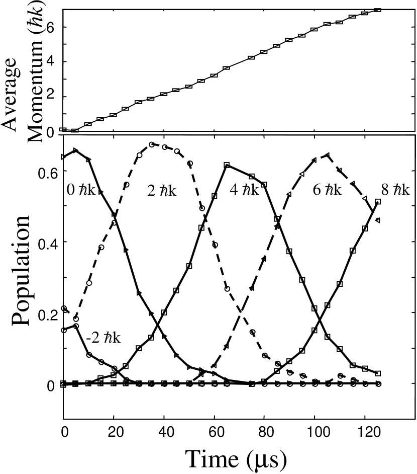
Figure 13: The momentum decomposition and mean momentum of a condensate in the lowest band after a period of constant acceleration. The acceleration sweeps the atoms through a Brillouin zone in 35$\mu$s. The reference frame is the stationary laboratory.

To obtain an accelerated BEC with a single momentum we turn the lattice off adiabatically. The BEC has a final momentum of $2m\hbar k$ where $m$ is the number of Brillouin zone boundaries crossed during the acceleration (i.e. the final lattice velocity is between $(2m-1)\hbar k/M$ and $(2m+1)\hbar k/M$.). We have accelerated a BEC up to momenta of 10$\hbar k$ (see figure 14 B). The final velocity is quite insensitive to power and frequency fluctuations in the lattice beams and to the specifics of the lattice acceleration. The limitations on our final velocity are purely technical: the range of the frequency sweep and the field of view of our camera.

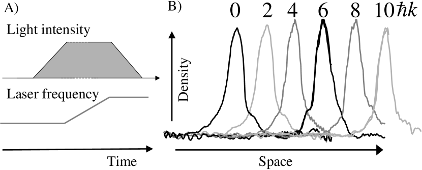
Figure 14: Accelerator for cold atoms. First the BEC is adiabatically loaded into the lattice ground state ($q=$0) and the lattice is subsequently accelerated (A). After sweeping through an integer number $m$ of Brillouin zones, the lattice is ramped down adiabatically, which results in a single BEC wavepacket moving at $2m\hbar k$. (B) shows accelerated BEC wavepackets with final momenta of up to 10$\hbar k$.

While there is no apparent limit on the final velocity there are limits on the acceleration. In our case the sudden initiation of the acceleration presents a limit as described above. If we adiabatically applied the acceleration to circumvent this limit there will always be the ultimate limit of “spilling”: when the acceleration is so large that there are no bound states.

6 A large-momentum-transfer beamsplitter

We now describe how we use the accelerator in order to build a coherent, large-momentum-transfer beamsplitter (LMT-beamsplitter). This is useful for applications that require atoms with large, coherent separations (in either position or momentum). A LMT-beamsplitter can be built using high-order Bragg diffraction [8], but is limited to relatively low momenta because the transition probability decreases rapidly with increasing order. Our approach is not limited in this way. It is similar in spirit to coherent beamsplitters based on adiabatic transfer [33, 34, 35].

Our scheme is outlined in figure 15: We begin with a second-order Bragg pulse [36, 8] that produces a coherent superposition of the two momentum states 0 and -4$\hbar k$. We use a $8E_{R}$ high lattice pulsed on for 6.4 $\mu$s at a velocity of $-2\hbar k/M$ to perform the splitting. We then adiabatically turn on a 14$E_{R}$ deep lattice at a velocity of $0.3\hbar k/M$. The lattice is accelerated to a velocity of approximately $2m\hbar k/M$ carrying the 0$\hbar k$ momentum component along with it. By contrast, the -4$\hbar k$ momentum component remains stationary.

Figure 15: A coherent, large-momentum, transfer beamsplitter. After splitting the condensate with a second-order Bragg pulse, a lattice moving at $0.3\hbar k/M$ is adiabatically turned on over 20 $\mu$s, such that the $0\hbar k$ and $-4\hbar k$ components are transferred into bands 0 and 4, respectively. The lattice is then accelerated over 200 $\mu$s. The component in band 0 accelerates with the lattice, while the component in band 2 stays at rest. After sweeping through $m$ Brillouin zone boundaries, the lattice is adiabatically turned off, resulting in two wavepackets, one with momentum -4$\hbar k$ and one with a momentum of $2m\hbar k$. In our experiments we swept through up to 4 Brillouin zone boundaries in about 200 $\mu$s.

The selective acceleration is achieved by choosing a lattice velocity such that the atoms with momentum 0$\hbar k$ in the lab frame are in band 0, while the atoms with -4$\hbar k$ are in band 4. Both have a quasimomentum of $-0.3\hbar k$. We chose this $q$ to ensure there are no degeneracies between bands at $V_{0}=0$ (see right hand side of figure 6).

As we accelerate the lattice, the atoms in band 0 are accelerated with the lattice, just as described in the previous section. Crossing the Brillouin zone boundary does not change the band. By contrast the atoms in band 4 respond as nearly free particles (since band 4 is unbound): when $q$ reaches the avoided crossing between bands 4 and 5 at the zone boundary (see figure 1) the atoms pass through to band 5 diabatically. At subsequent level crossings (such as for bands 5 and 6 at $q=0$) this process continues. In the lab frame this corresponds to the atoms being unaccelerated.

We can apply the Landau-Zener criterion for diabatic passage through the avoided crossings. The probability for a passage between bands $(n-1)$ and $n$ is [37] :

$$P_{\mathrm{LZ}}=\exp{\left\{-\pi\frac{\omega^{2}}{4\,n\,k\,a}\right\}},$$ (10)

where $\omega$ is the band gap frequency. This expression is derived in the limit where the anti-crossings are small. For the passage from bands 4 to 5 the gap is 2.2 kHz, giving a diabatic probability of 99.8% for our acceleration of $a=1200$ m$\cdot$s^-2. (If we had used a first-order Bragg pulse to initially split the condensate into 0 and 2$\hbar k$ components, then only 72% of the population would have passed through the first crossing.)

We end the experiment by adiabatically ramping down the intensity of the moving lattice. We get two wave packets, one at $2m\hbar k$ (recall that $m$ is the number of Brillouin zone boundaries crossed), the other at rest. We have demonstrated splittings of up to 12$\hbar k$.

The LMT-beamsplitter can be used to construct an interferometer. We have performed a proof-of-principle experiment in which we have built a Mach-Zehnder interferometer similar to that described in [38, 39]. In our case the initial Bragg pulse beamsplitter was replaced with the LMT-beamsplitter and the final Bragg pulse beamsplitter with a time-reversed version of the LMT-beamsplitter. In addition the Bragg $\pi$-pulse of the conventional Mach-Zehnder interferometer is replaced with a three stage LMT-$\pi$-pulse consisting of a deceleration stage, a conventional Bragg $\pi$-pulse and a final acceleration stage. The resulting interference pattern had a contrast of 50%, which was limited by transverse motion of the BEC during the experiment.

7 Conclusions

In conclusion, we have performed a number of experiments with a BEC in static, moving, and accelerating 1D optical lattices and have interpreted the results using band structure. We have studied adiabatic loading into the ground state and coherent transfer to other lattice states by modulating the lattice. These techniques have been used to perform band spectroscopy. We have also built an coherent accelerator and a multiphoton beamsplitter.

During preparation of this paper we learned of several other optical lattice experiments with a BEC [12, 13, 14, 15, 16, 18].

References

References

- [1] M. H. Anderson, J. R. Ensher, M. R. Matthews, C. E. Wieman, and E. A. Cornell. Science, 269:198, 1995.
- [2] K. B. Davis, M.-O. Mewes, M. R. Andrews, N. J. van Druten, D. S. Durfee, D. M. Kurn, and W. Ketterle. Phys. Rev. Lett., 75:3969, 1995.
- [3] J.P. Dowling and J. Gea-Banacloche. Adv. At. Mol. Opt. Phys., 37:1, 1996.
- [4] R. Grimm and M. Weidemüller. Optical dipole traps for neutral atoms. Adv. At. Mol. Opt. Phys., 42:95, 2000.
- [5] S. Bernet, R. Abfalterer, C. Keller, M. K. Oberthaler, J. Schmiedmayer, and A. Zeilinger. Phys. Rev. A, 62:023606, 2000.
- [6] B.P. Anderson and M. A. Kasevich. Science, 282:1686, 1998.
- [7] Yu. B. Ovchinnikov, J. H. Müller, M. R. Doery, E. J. D. Vredenbregt, K. Helmerson, S. L. Rolston, and W. D. Phillips. Phys. Rev. Lett., 83:284, 1999.
- [8] M. Kozuma, L. Deng, E. W. Hagley, J. Wen, R. Lutwak, K. Helmerson, S. L. Rolston, and W. D. Phillips. Phys. Rev. Lett., 82:871, 1999.
- [9] J. Stenger, S. Inouye, A. P. Chikkatur, D. M. Stamper-Kurn, D. E. Pritchard, and W. Ketterle. Phys. Rev. Lett., 82:4569, 1999.
- [10] L. Deng, E. W. Hagley, J. Denschlag, J. E. Simsarian, M. Edwards, C. W. Clark, K. Helmerson, S. L. Rolston, and W. D. Phillips. Phys. Rev. Lett., 83:5407, 1999.
- [11] W. K. Hensinger, H. Häffner, A. Browaeys, N. R. Heckenberg, K. Helmerson, C. McKenzie, G. J. Milburn, W. D. Phillips, S. L. Rolston, H. Rubinsztein-Dunlop, and B. Upcroft. Nature, 412:52, 2001.
- [12] O. Morsch, J. H. Müller, M. Cristiani, D. Ciampini, and E. Arimondo E. Phys. Rev. Lett., 87:140402, 2001.
- [13] F. S. Cataliotti, S. Burger, C. Fort, P. Maddaloni, F. Minardi, A. Trombettoni, A. Smerzi, and M. Inguscio. Science, 293:843, 2001.
- [14] P. Pedri, L. Pitaevskii, S. Stringari, C. Fort, S. Burger, F. S. Cataliotti, P. Maddaloni, F. Minardi, and M. Inguscio. Phys. Rev. Lett., 87:220401, 2001.
- [15] S. Burger, F. S. Cataliotti, C. Fort, F. Minardi, M. Inguscio, M. L. Chiofalo, and M. P. Tosi. Phys. Rev. Lett., 86:4447, 2001.
- [16] M. Greiner, I. Bloch, O. Mandel, T. W. Hänsch, and T. Esslinger. Phys. Rev. Lett, 87:160405, 2001.
- [17] C. Orzel, A. K. Tuchman, M. L. Fenselau, M. Yasuda, and M. A. Kasevich. Science, 291:2386, 2001.
- [18] M. Greiner, O. Mandel, T. Esslinger, T. W. Hänsch, and I. Bloch. Nature, 415:39, 2002.
- [19] K. Berg-Sørensen and K. Mølmer. Phys. Rev. A, 58:1480, 1998.
- [20] D. Jaksch, C. Bruder, J. I. Cirac, C. W. Gardiner, and P. Zoller. Phys. Rev. Lett., 81:3108, 1998.
- [21] D. Choi and Q. Niu. Phys. Rev. Lett., 82:2022, 1999.
- [22] M. Holthaus. J. Opt. B, 2:589, 2000.
- [23] M. L. Chiofalo, M. Polini, and M. P. Tosi. Eur. Phys. J. D, 11:371, 2000.
- [24] S. Pötting, M. Cramer, C. H. Schwalb, H. Pu, and P. Meystre. Phys. Rev. A, 64:023604, 2001.
- [25] J. C. Bronski, L. D. Carr, B. Deconinck, and J. N. Kutz. Phys. Rev. Lett., 86:1402, 2001.
- [26] M. Ben Dahan, E. Peik, J. Reichel, Y. Castin, and C. Salomon. Phys. Rev. Lett., 76:4508, 1996.
- [27] E. Peik, M. Ben Dahan, I. Bouchoule, Y. Castin, and C. Salomon. Phys. Rev. A, 55:2989, 1997.
- [28] S. R. Wilkinson, C. F. Bharucha, K. W. Madison, Qian Niu, and M. G. Raizen. Phys. Rev. Lett., 76:4512, 1996.
- [29] W. Petrich, M. H. Anderson, J. R.Ensher, and E. A. Cornell. Phys. Rev. Lett., 74:3352, 1995.
- [30] F. Dalfovo, S. Giorgini, L. P. Pitaevskii, and S. Stringari. Rev. Mod. Phys., 71:463, 1999.
- [31] H. J. Metcalf and P. van der Straten. Laser Cooling and Trapping. Springer, 1999.
- [32] L. Schiff. Quantum Mechanics. McGraw Hill, third edition, 1968.
- [33] J. Lawall and M. Prentiss. Phys. Rev. Lett., 72:993, 1994.
- [34] L. S. Goldner, C. Gerz, R. J. C. Spreeuw, S. L. Rolston, C. I. Westbrook, W. D. Phillips, P. Marte, and P. Zoller. Phys. Rev. Lett., page 997, 1994.
- [35] M. Weitz, B. C. Young, and S. Chu. Phys. Rev. A, 50:2438, 1994.
- [36] P. J. Martin, B. G. Oldaker, A. H. Miklich, and D. E. Pritchard. Phys. Rev. Lett., 60:515, 1988.
- [37] G. Zener. Proc. R. Soc. London A, 137:696, 1932.
- [38] J. Denschlag, J. E. Simsarian, D. L. Feder, C. W. Clark, L. A. Collins, J. Cubizolles, L. Deng, E. W. Hagley, K. Helmerson, W. P. Reinhardt, S. L. Rolston, B. I. Schneider, and W. D. Phillips. Science, 287:97, 1999.
- [39] Y. Torii, Y. Suzuki, M. Kozuma, T. Sugiura, T. Kuga, L. Deng, and E. W. Hagley. Phys. Rev. A, 61:041602, 2000.