The idea of using Josephson junctions as sources of electromagnetic radiation is promising owing to their small dimensions, good tunability, and capability of operating at frequencies up to several hundred gigahertz [1]. However, the power of radiation available from a single junction is not sufficient for most applications, which necessitates using arrays of junctions. A stack arrangement of long Josephson junctions (LJJs) [2] arouses interest because of possible improvements of the properties of LJJ oscillators in terms of impedance matching, output power, and integration level. The low-$T_{c}$ superconductor thin film technology allows growth of high-quality multilayers with many Josephson tunnel barriers (for example, Nb/Al-${\rm AlO_{x}}$/Nb) stacks). Moreover, the discovery of an intrinsic Josephson effect in some high-$T_{c}$ superconductors such as BSCCO convincingly showed that these materials are essentially natural superlattices of LJJs formed on the atomic scale [3]. Recent theoretical investigations and experiments showed that the inductive coupling between adjacent junctions leads to diverse and nontrivial dynamic behaviour patterns of such structures [4, 5, 6, 7].

One possible way to produce coherent radiation from stacks of LJJs is to form a regular Josephson vortex lattice (JVL) and move it by an external current. In order to produce maximum radiation from a stack at a given lattice velocity and external magnetic field, a rectangular arrangement of vortices, when vortices in neighboring layers are located one over another, is most preferable. Such a lattice is feasible provided the corresponding solution is stable. In the present paper we show that in a two-junction stack a rectangular JVL is unstable at low velocities, and stability of such a solution can be achieved at high velocities of JVL, provided there is a large external magnetic field, or large enough damping, or small stack length. Specifically, the above conditions may explain the results of numerical [4, 5, 6] and experimental [7] investigations in which a possibility of existence of rectangular JVL in stacks of two and more LJJs is shown. Our result complements the results reported in [8] where the authors argue that a rectangular JVL is stable at high velocities in an infinite stack. The incompleteness of this result is explained by the fact that the authors of [8] have not taken into account all possible perturbations of the solution in the form of a rectangular JVL.

Let us consider the set of equations describing a simplest layered structure — a stack consisting of two LJJs with magnetic coupling between the layers [2, 8, 9]:

$$\partial^{2}_{x}(\varphi_{1,2}+\eta\varphi_{2,1})=(\partial^{2}_{t}+\gamma\partial_{t})\varphi_{1,2}+\sin\varphi_{1,2}-j.$$ (1)

Here $\varphi_{1,2}$, $\gamma$, $j$ are the Josephson phase difference, damping constant, and bias current density, respectively. The magnetic coupling parameter is denoted by $\eta$. It is determined by the formula [2]:

$$\eta=\lambda(d\sinh{\frac{t}{\lambda}}+2\lambda\coth{\frac{t}{\lambda}})^{-1},$$ (2)

where $\lambda$ is the London penetration depth, $t$ is the thickness of the superconducting layer, $d$ is the distance between two superconducting layers. We start with the assumption that the system is infinite in space.

To investigate a two-junction stack it is convenient to introduce new variables $\varphi_{\pm}=(\varphi_{1}\pm\varphi_{2})/2$, which obey the set of equations:

$$c^{2}_{\pm}\partial^{2}_{x}\varphi_{\pm}=(\partial^{2}_{t}+\gamma\partial_{t})\varphi_{\pm}+\sin\varphi_{\pm}\cos\varphi_{\mp}-j_{\pm},$$ (3)

where $c^{2}_{+}=1$, $c^{2}_{-}=(1-\eta)/(1+\eta)$, $j_{+}=j$, $j_{-}=0$. We have renormalized the coordinate $x_{new}=x_{old}/\sqrt{1+\eta}$ in Eqs. (3).

The set of Eqs. (3) has a solution describing rectangular JVL. Assuming the external magnetic field to be high we can write down the analytical expressions for this solution [10]:

$$\varphi_{+}^{0}=h(x-ut)+{\rm Im}\frac{e^{ih(x-ut)}}{L},\quad\varphi_{-}^{0}\equiv 0,$$ (4)

where $L=-h^{2}(1-u^{2})+i\gamma uh$, $u$ is the JVL velocity, $h\gg 1$ is the dimensionless external magnetic field. Velocity $u$ and damping $\gamma$ are related through the energy balance condition [11] which is actually the current-voltage characteristic of the stack with the rectangular JVL:

$$j=-\gamma uh+\frac{1}{2}{\rm Im}\frac{1}{L}.$$ (5)

We note that the solution in the form (4) is valid only provided $|L^{-1}|\ll 1$. If $h\gamma\gg 1$ the previous condition is satisfied at all velocities otherwise it breaks in a region near $u=1$. This region corresponds to the peak in the current-voltage characteristic (5).

In order to investigate the stability of rectangular JVL we search for the solution of (3) in the form $\varphi_{\pm}=\varphi_{\pm}^{0}+\delta\varphi_{\pm}$ where $\varphi_{\pm}^{0}$ are given by (4) and $\delta\varphi_{\pm}$ are small perturbations ($|\delta\varphi_{\pm}|\ll 1$). Substituting this solution into (3) and neglecting the terms nonlinear in $\delta\varphi_{\pm}$ we obtain:

$$c^{2}_{\pm}\partial^{2}_{x}\delta\varphi_{\pm}=(\partial^{2}_{t}+\gamma\partial_{t})\delta\varphi_{\pm}+\cos{\varphi_{+}^{0}}\cdot\delta\varphi_{\pm},$$ (6)

where $\cos{\varphi_{+}^{0}}\approx\cos{h(x-ut)}+{\rm Re}((1-e^{2ih(x-ut)})/2L)$. We will refer to $\delta\varphi_{+}$ and $\delta\varphi_{-}$ as symmetrical and antisymmetrical perturbations, respectively. The set (6) is actually two independent equations so we can analyze them separately. Thus we have divided the problem of rectangular JVL stability into two ones — the problems of stability with respect to symmetrical and antisymmetrical perturbations.

We start with an analysis of the ”subluminal” ($u<1$) solution stability. The problem of a rectangular JVL stability with respect to symmetrical perturbations is similar to the problem of stability of the periodical vortex chain in LJJ which was solved in [10]. Thus a ”subluminal” rectangular JVL is stable to symmetrical perturbations. To analyze the stability of (4) with respect to antisymmetrical perturbations we use Eq. (6) for $\delta\varphi_{-}$. This equation is a relativistic invariant with $c_{-}$ being the characteristic velocity of antisymmetrical perturbation. From (2) and the expression for $c_{-}$ it is seen that $c_{-}<1$ at any stack parameters. In other words, antisymmetrical perturbations are always slow compared with the symmetrical ones. Therefore, to investigate the ”subluminal” solution stability it is necessary to distinguish between two cases: $u<c_{-}$ and $u>c_{-}$.

Let us first consider the case $u<c_{-}$. We perform the Lorentz transformation in Eq. (6) for $\delta\varphi_{-}$:

$$\xi=\frac{x-vt}{\sqrt{1-(v/{c_{-}})^{2}}},\qquad\tau=\frac{t-(v/c^{2}_{-})x}{\sqrt{1-(v/{c_{-}})^{2}}}$$

with velocity $v=u$. Introducing $\psi\equiv\delta\varphi_{-}$ we obtain the equation

$$c^{2}_{-}\psi_{\xi\xi}=\psi_{\tau\tau}+\frac{\gamma}{\sqrt{1-(u/c_{-})^{2}}}(\psi_{\tau}-u\psi_{\xi})+\cos{\varphi_{+}^{0}}\cdot\psi$$

where the parameter depends only on the coordinate $\xi$. After the renormalization of the coordinate $h\sqrt{1-(u/c_{-})^{2}}\xi_{old}=2\xi_{new}$ and time $h\sqrt{1-(u/c_{-})^{2}}\tau_{old}=2\tau_{new}$ and introduction of the small parameter $\mu=4h^{-2}(c_{-}^{2}-u^{2})^{-1}$ we have:

$$\psi_{\xi\xi}+\Gamma_{\xi}\psi_{\xi}=\frac{1}{c_{-}^{2}}(\psi_{\tau\tau}+\Gamma_{\tau}\psi_{\tau})+\mu[\cos{2\xi}+{\rm Re}\frac{1-e^{4i\xi}}{2L}]\psi,$$ (7)

where $\Gamma_{\xi}=\mu hu\gamma/2$, $\Gamma_{\tau}=\mu h\gamma c_{-}^{2}/2$. We look for the solution of (7) in the form of the Fourier integral $\psi(\xi,\tau)=\int_{-\infty}^{\infty}\tilde{\psi}(\xi,\omega)e^{-i\omega\tau}\frac{d\omega}{2\pi}$. The equation for the Fourier image of $\psi(\xi,\tau)$ is

$$\tilde{\psi}_{\xi\xi}+\Gamma_{\xi}\tilde{\psi}_{\xi}=-\frac{\omega^{2}+i\omega\Gamma_{\tau}}{c_{-}^{2}}\tilde{\psi}+\mu[\cos{2\xi}+{\rm Re}\frac{1-e^{4i\xi}}{2L}]\tilde{\psi}.$$ (8)

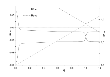
Figure 1: Eigenfrequency $\omega(q)$ spectrum as a function of quasimomentum $q$ for antisymmetric perturbations (case $u<c_{-}$)

According to the Bloch theorem, the solutions of (8) have the form $\tilde{\psi}(\xi)=\exp{(iq\xi)}U_{q}(\xi)$, where $q$ is the quasimomentum and $U_{q}(\xi)$ is the function with the period $\pi$. Let us find the eigenfrequency spectrum $\omega(q)$. At $\mu=0$ the spectrum is

$$\omega(\omega+i\Gamma_{\tau})=c_{-}^{2}q(q-i\Gamma_{\xi}).$$ (9)

At $\mu\neq 0$ the maximum perturbations of the spectrum are achieved near the middle point ($q=0$) and the edges ($q=\pm 1$) of the first Brillouin zone. In the vicinity of $q=0$ we search for the solution of (8) in the form

$$\tilde{\psi}(\xi)=e^{iq\xi}[a_{0}+a_{2}e^{2i\xi}+a_{-2}e^{-2i\xi}],$$

where $a_{0},a_{\pm 2}$ are constants. After substituting it into (8) we obtain the dispersion characteristic as the condition for $a_{0,\pm 2}$ at which the solution of (8) is not equal to zero:

$$-(q-\frac{i\Gamma_{\xi}}{2})^{2}+c_{-}^{-2}(\omega+\frac{i\Gamma_{\tau}}{2})^{2}-\mu\alpha=-\frac{\mu^{2}}{8},$$ (10)

where $\alpha={\rm Re}\,(2L)^{-1}-\gamma^{2}/4$. Near $q=1$ the solution has the form

$$\tilde{\psi}(\xi)=e^{i(q-1)\xi}[a_{1}e^{i\xi}+a_{-1}e^{-i\xi}],$$

where $a_{\pm 1}$ are constants. Substitution of this expression into (8) gives

$$(\frac{\omega+i\Gamma_{\tau}/2}{c_{-}}-\frac{\mu\alpha}{2}-1)^{2}-(q-\frac{i\Gamma_{\xi}}{2}-1)^{2}=\frac{\mu^{2}}{16}.$$ (11)

Far from the middlepoint and the edges of the first Brillouin zone the spectrum remains unperturbed and is given by the formula (9).

The dependencies of real and imaginary parts of eigenfrequency $\omega(q)$ are shown in Fig.1. It is seen that at small $q$ some roots of the dispersion equation (10) have positive imaginary parts. This means that perturbations with small $q$ will exponentially grow with time, i.e. the solution (4) is unstable. We see that the instability which is obvious in the case of low density chains (due to repulsion of vortices in the neighbouring layers) is not changed by stability in the case of denser chains. This result is in agreement with the one obtained in [8] and reflects the fact that the vortex chains in the neighbouring layers tend to shift and form the triangular JVL.

Let us now consider the case of high velocities $c_{-}<u<1$. As before, we perform the Lorentz transformation in Eq. (6) for $\delta\varphi_{-}$ but now with the velocity $v=c^{2}_{-}/u$. Introducing $\psi\equiv\delta\varphi_{-}$ we obtain the equation

$$c^{2}_{-}\psi_{\xi\xi}=\psi_{\tau\tau}+\frac{\gamma}{\sqrt{1-(c_{-}/u)^{2}}}(\psi_{\tau}-\frac{c_{-}^{2}}{u}\psi_{\xi})+\cos{\varphi_{0}^{+}}\cdot\psi,$$

where the parameter depends only on the time $\tau$. This equation turns into

$$\psi_{\tau\tau}+\Gamma_{\tau}\psi_{\tau}=c_{-}^{2}(\psi_{\xi\xi}+\Gamma_{\xi}\psi_{\xi})-\mu(\cos{2\tau}+{\rm Re}\frac{1-e^{4i\tau}}{2L})\psi,$$ (12)

where $h\sqrt{u^{2}-c_{-}^{2}}\tau_{old}=2\tau_{new}$, $h\sqrt{u^{2}-c_{-}^{2}}\xi_{old}=2\xi_{new}$, $\mu=4h^{-2}(u^{2}-c_{-}^{2})^{-1}$, $\Gamma_{\tau}=\mu uh\gamma/2$, $\Gamma_{\xi}=\mu h\gamma/2$. We look for the solution of (12) in the form of the Fourier integral $\psi(\xi,\tau)=\int_{-\infty}^{\infty}\tilde{\psi}(k,\tau)e^{-ik\xi}\frac{dk}{2\pi}$. The equation for the Fourier image of $\psi(\xi,\tau)$ is

$$\tilde{\psi}_{\tau\tau}+\Gamma_{\tau}\tilde{\psi}_{\tau}=-c_{-}^{2}(k^{2}-ik\Gamma_{\xi})\tilde{\psi}-\mu(\cos{2\tau}+{\rm Re}\frac{1-e^{4i\tau}}{2L})\tilde{\psi}.$$ (13)

The solution of (13) has the form $\tilde{\psi}(\tau)=\exp{(-i\varepsilon\tau)}U_{\varepsilon}(\tau)$ where $\varepsilon$ is the quasienergy and $U_{\varepsilon}(\tau)$ is the function with the period $\pi$. Let us find the spectrum $\varepsilon(k)$ by the scheme used above. In the vicinity of $\varepsilon=0$ the spectrum is

$$-(\varepsilon+\frac{i\Gamma_{\tau}}{2})^{2}+c_{-}^{2}(k-\frac{i\Gamma_{\xi}}{2})^{2}+\mu\alpha=-\frac{\mu^{2}}{8},$$ (14)

and near $\varepsilon=1$:

$$(c_{-}(k-\frac{i\Gamma_{\xi}}{2})+\frac{\mu\alpha}{2}-1)^{2}-(\varepsilon+\frac{i\Gamma_{\tau}}{2}-1)^{2}=\frac{\mu^{2}}{16}.$$ (15)

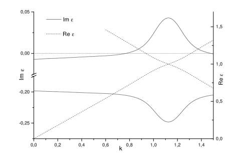
Figure 2: Quasienergy $\varepsilon(k)$ as a function of wavenumber $k$ for antisymmetric perturbations (case $c_{-}<u<1$)

It follows from the Eq. (15) that at certain $k$ the roots of the dispersion equation may have positive imaginary part as it is shown in Fig.2. ${\rm Im}\,\varepsilon(k)$ reaches its maximum value at $k=c_{-}^{-1}$. At small $\gamma$ $({\rm Im}\,\varepsilon(k))_{max}\approx\mu/4-\Gamma_{\tau}/2$. Therefore, the perturbation with $k=c_{-}^{-1}$ depends on time like

$$\tilde{\psi}(k,\tau)\sim\exp{[(\frac{\mu}{4}-\frac{\Gamma_{\tau}}{2})\tau_{new}}]=\exp{[\frac{(h^{-1}-u\gamma)\tau_{old}}{2\sqrt{u^{2}-c_{-}^{2}}}]}.$$

It is seen from this expression that the solution (4) is either stable or unstable depending on sign of the difference $h^{-1}-u\gamma$. If $hu\gamma<1$ the solution (4) is parametrically unstable. The region of $k$ corresponding to the growing perturbations is equal to

$$\Delta k\approx\frac{2}{c_{-}}\sqrt{\frac{\mu^{2}}{16}-\frac{\Gamma_{\tau}^{2}}{4}}.$$ (16)

This parametric instability may be ”suppressed” either by increasing the external magnetic field $h$ or by increasing the damping $\gamma$. We would like to emphasize that the instability appears due to the periodicity of the solution. Therefore the results obtained in [12] for the isolated vortices cannot be applied to the case of periodic vortex chains.

It remains to investigate the stability of the ”superluminal” JVL ($u>1$). We start with the analysis of the stability with respect to symmetrical perturbations. Substituting the solution (4) into Eq. (6) for $\delta\varphi_{+}$ and applying the Lorentz transformation

$$\xi=\frac{x-vt}{\sqrt{1-v^{2}}},\qquad\tau=\frac{t-vx}{\sqrt{1-v^{2}}}$$

with $v=u^{-1}$, we obtain

$$\psi_{\xi\xi}=\psi_{\tau\tau}+\frac{\gamma}{\sqrt{1-(1/u)^{2}}}(\psi_{\tau}-\frac{1}{u}\psi_{\xi})+\cos{\varphi_{0}^{+}}\cdot\psi,$$ (17)

where $\psi\equiv\delta\varphi_{+}$. In this equation the coefficient at $\psi$ depends only on time $\tau$ and is periodical. Analyzing this equation by the method used for the case $c_{-}<u<~{}1$ we arrive at the conclusion that there are shortwave perturbations which depend exponentially on time $\tau$ and the solution (4) may be stable or unstable depending on sign of the difference $h^{-1}-u\gamma$. The same result is obtained also for the antisymmetric perturbations in the case $u>1$. The main feature of this result is that the stability condition $h^{-1}<u\gamma$ may be achieved by increase of $u$. However, the alternate component of the electric field $\varphi_{t}$ of such a solution has the order $h^{-1}u(u^{2}-1)^{-1}$ and is small. Therefore, the power of radiation from the edge of the stack in this case is not sufficient for applications in spite of the fact that the JVL is rectangular.

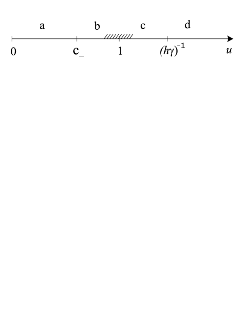
Figure 3: Stability diagram for the rectangular vortex lattice (case $h\gamma<1$). Latin letters mark the regions of different behaviour of small perturbations: a – longwave instability, b – shortwave instability to antisymmetric perturbations, c – shortwave instability to both symmetric and antisymmetric perturbations, d – stability. Hatching shows the region where the solution (4) is not valid.

Combining the results obtained above we build the diagram (Fig. 3) showing the regions of stability and instability in terms of the lattice velocity $u$. At $0<u<c_{-}$ the solution (4) is unstable with respect to longwave perturbations and formation of the triangular JVL. At $c_{-}<u<(h\gamma)^{-1}$ the solution is unstable due to the parametric resonance and the instability growth rate is proportional to $h^{-1}-u\gamma$. In the region near $u=1$ where the condition $|L^{-1}|\ll 1$ breaks the solution (4) is not valid and more thorough investigation is required. Then, at $u>(h\gamma)^{-1}$ the parametric resonance is ”suppressed” and the solution becomes stable. The diagram Fig. 3 is built for the case $h\gamma<1$. When $h\gamma>1$ the instability region is $0<u<(h\gamma)^{-1}$. At last, when $(h\gamma)^{-1}<c_{-}$ the instability region is $0<u<c_{-}$.

Consider now the case when the system is not infinite in space. The simplest way to change to a finite system is to set periodic boundary conditions

$$\varphi_{1,2}(x=l,t)=\varphi_{1,2}(x=0,t)+2\pi N,$$

where $N$ is the number of vortices trapped in each junction of the stack, $l$ is the length of the system. The boundary conditions for perturbations are written as below:

$$\delta\varphi_{\pm}(\xi_{new}=hl/2,\tau)=\delta\varphi_{\pm}(\xi_{new}=0,\tau).$$ (18)

At $u<c_{-}$ the conditions (18) lead to discreteness of quasimomentum $q$ with the step $4\pi/hl$. As the instability interval is located near $q=0$, mode with $q=0$ will always be in this interval, i.e. it will grow with time. Hence, the periodic boundary conditions cannot provide stability of a rectangular JVL at small velocities. At $c_{-}<u<1$ the wavenumber $k$ is discrete with the step $4\pi/hl$. At large $l$ when $\Delta k>4\pi/hl$ at least one of the possible values of $k$ will be in the interval of instability (16), therefore, the solution will be unstable at $h^{-1}>u\gamma$. The necessary condition of stability is

$$l>\pi hc_{-}(c_{-}^{2}-u^{2}).$$

This means that to provide a rectangular JVL stability at $c_{-}<u<1$ it is necessary to decrease the system length $l$ so that no permitted value of $k$ is in the interval (16). At $1<u<(h\gamma)^{-1}$ the situation is more complicated because the instability intervals in $k$ have different widths and are differently located for symmetrical and antisymmetrical perturbations. But it is clear that the decrease of $l$ lowers the number of permitted $k$ in the instability intervals and may lead to stability.

Let us summarize the obtained results. At low velocities a rectangular JVL in an infinite two-junction stack is unstable with respect to perturbations with scales much larger than the lattice period. The physical meaning of this is that the vortex chains in the first and second junctions tend to shift with respect to each other to compose a triangular JVL. This is in agreement with the result of [8]. At high but ”subluminal” velocities the lattice may be unstable with respect to perturbations with scales comparable to the period of the JVL. The growth rate of this parametric instability is determined by the difference $h^{-1}-u\gamma$ and, therefore, the instability may be ”suppressed” by high enough external magnetic field, or by the damping in the system, or by the increase of the lattice velocity. The existence of this instability complements the results obtained in [8] where the authors did not take into account the short-wave perturbations. In the present paper we also show that the stability of rectangular JVL at low damping is possible in a finite two-junction stack. Thus we argue that the formation of a rectangular JVL which is reported in [4, 5, 6, 7] is associated either with the finiteness of the system or with the suppression of the instability by three ways mentioned above.

This work was supported by the Russian Foundation for Fundamental Research (Grant No. 00-02-16528). The authors are grateful to N. Gress for assistance in the preparation of the English version of the manuscript.

References

- [1] A. Barone and G. Paternò, ”Physics and Applications of the Josephson Effect”, 1982.
- [2] S. Sakai, P. Bodin, and N.F. Pedersen, J. Appl. Phys. 73, 2411 (1993).
- [3] R. Kleiner, F. Steinmeyer, G. Kunkel, and P. Müller, Phys. Rev. Lett. 68, 2394, (1992); R. Kleiner and P. Müller, Phys. Rev B 49, 1327, (1994).
- [4] A. Petraglia, A.V. Ustinov, N.F. Pedersen, and S. Sakai, J. Appl. Phys. 77, 1171 (1995).
- [5] M. Machida, T. Koyama, A. Tanaka, and M. Tachiki, Physica C 330, 85, (2000).
- [6] A.V. Ustinov and S. Sakai, Appl. Phys. Lett. 73, 686 (1998).
- [7] S.V. Shitov, A.V. Ustinov, N. Iosad, and H. Kohlstedt, J. Appl. Phys. 80, 7134 (1996).
- [8] A.F. Volkov and V.A. Glen, J. Phys.: Condens. Matter 10, L563, (1998); A.E. Koshelev and I.S. Aranson, Phys. Rev. Lett. 85, 3938, (2000); S.N. Artemenko and S.V. Remizov, Physica C 362, 200 (2001).
- [9] L.N. Bulaevskii, M. Zamora, D. Baeriswyl, H. Beck, and J.R. Clem, Phys. Rev B 50, 12831, (1994).
- [10] P. Lebwohl and M.J. Stephen, Phys. Rev. 163, 376 (1967).
- [11] D.W. McLaughlin and A.C. Scott, Phys. Rev A 18, 1652 (1978).
- [12] N. Grønbech-Jensen et al., Phys. Rev. B 48, R16160, ibid 50, 6352.