JOURNAL OF THE PHYSICAL SOCIETY OF JAPAN 67 (1998) 3867-3874
Off-diagonal Wave Function Monte Carlo Studies of Hubbard Model I

Abstract

We propose a Monte Carlo method, which is a hybrid method of the quantum Monte Carlo method and variational Monte Carlo theory, to study the Hubbard model. The theory is based on the off-diagonal and the Gutzwiller type correlation factors which are taken into account by a Monte Carlo algorithm. In the 4$\times$4 system our method is able to reproduce the exact results obtained by the diagonalization. An application is given to investigate the half-filled band case of two-dimensional square lattice. The energy is favorably compared with quantum Monte Carlo data.

Key words: Hubbard model, Monte Carlo method, off-diagonal function

I Introduction

Strongly correlated electron systems have been investigated by many researchers in order to understand the mechanism of superconductivity of the high-T_c oxide superconductors. The effect of strong correlation between electrons is important for high-T_c superconductivity and many unconventional phenomena such as metal-insulator transition and heavy fermions with a huge large mass. The Hubbard model is a basic model for strongly correlated electrons in metals. The Hubbard model has been regarded as a model to describe the Mott transition in compounds such as NiO and MnO.^? It is considered that the Hubbard model contains basic physics of high-T_c superconductivity as a simplified one-band model of the three band Cu-O model.^? A possibility of superconductivity for the 2D Hubbard model has been controversial for many years.^??? The study of the Hubbard model provides us insights having important implications concerning the origin of high-T${\rm c}$ superconductivity. The possibility of the superconducting state is recently reported for the Hubbard model^???? and the two-chain Hubbard model.^??? The phase diagram is still far from well understood in two dimensions.

The quantum Monte Carlo method is a method to treat the strong correlations exactly. However, the applicability is restricted to moderately correlated region because of a sign problem. The variational Monte Carlo method has a feature characterized by a wide applicability from weak to strong correlation. The Gutzwiller wave function is a standard trial wave function for itinerant correlated electrons. In the Gutzwiller function only the correlation at the same site is taken into account and thus the wave function is very simple in its form. An analytic evaluation of expectation values is, however, very difficult for the Gutzwiller function in spite of its simplicity. This difficulty is overcome by a Monte Carlo method and many calculations have been performed using the Monte Carlo algorithm.^????

It is revealed that the Gutzwiller function will give higher energies compared to exact values. Thus we think that the Gutzwiller function should be improved to investigate the ground state more precisely. The purpose of this paper is to propose a hybrid method of the quantum Monte Carlo (QMC) calculations and variational Monte Carlo (VMC) theory. Following an idea of QMC, a trial function is improved and the expectation values of energy and other quantities are calculated using VMC for the parameters optimizing the energy expectation value. The off-diagonal wave function Monte Carlo method (OWMC) in this paper deal with Gutzwiller projection and off-diagonal correlation operators taken into account by a Monte Carlo algorithm. We expect to be able to extrapolate correct expectation values from the data obtained for off-diagonal wave functions.

We show advantages of OWMC in the following: (1) The calculations give an upper bound of the exact energy since OWMC is based on the variational theory. (2) Variational wave functions are improved systematically. (3) There is no sign problem. (4) The large-$U$ systems are tractable. (5) Introducing the order parameters we can investigate ground state properties characterized by the long-range ordering.

The paper is organized as follows. The section 2 is devoted to present the Hamiltonian and wave functions. The method of calculations is also shown. The following two sections are assigned to a description of results. The summary and discussion are presented in the final section.

II Hamiltonian and wave functions

A Wave functions

The Hamiltonian is given by the Hubbard model:

$$H=-t\sum_{\langle ij\rangle}(c^{{\dagger}}_{i\sigma}c_{j\sigma}+{\rm h.c.})+U\sum_{i}n_{i\uparrow}n_{i\downarrow},$$ (1)

where $n_{i\sigma}=c^{{\dagger}}_{i\sigma}c_{i\sigma}$ is the number operator and $U$ is the strength of on-site Coulomb interaction. The energy is measured in units of $t$ throughout this paper and the number of sites is denoted as $N$. In this paper the Hubbard model is considered in two space dimensions. The Coulomb interaction $U$ is expected to bring about the metal-insulator transition, antiferromagnetic order and a possibility of the anisotropic superconducting state.

Let us start with the Gutzwiller function given by

$$\psi_{G}=P_{G}\psi_{0}={\rm exp}(-\alpha\sum_{i}n_{i\uparrow}n_{i\downarrow})\psi_{0}\equiv\psi^{(0)},$$ (2)

where $\psi_{0}$ is the free fermion ground state. $P_{G}$ is the Gutzwiller operator given by $P_{G}=\prod_{i}(1-(1-g)n_{i\uparrow}n_{i\downarrow})$ where $g$ is the variational parameter in the range of $0\leq g\leq 1$ and $\alpha={\rm log}(1/g)$. Our method is based on the fact that the ground state eigenfunction is written as in QMC

$$\psi=e^{-\beta H}\psi_{0}\simeq e^{-\epsilon_{1}K}e^{-\epsilon_{1}V^{\prime}}\cdots e^{-\epsilon_{n}K}e^{-\epsilon_{n}V^{\prime}}\psi_{0},$$ (3)

for large $\beta=\epsilon_{1}+\cdots+\epsilon_{n}$ and small $\epsilon_{i}$ ($i=1,\cdots,n$). $H$ is written as $H=K+V^{\prime}$ where $K$ denotes the kinetic energy part and $V^{\prime}=UV$ denotes the on-site interaction part: $V=\sum_{i}n_{i\uparrow}n_{i\downarrow}$. Since the last factor $e^{-\epsilon V^{\prime}}\psi_{0}$ in eq.(3) is regarded as the Gutzwiller function, one way to improve $\psi_{G}$ is achieved by multiplying $e^{-\lambda K}$ to $\psi_{G}$. Therefore we can consider^?

$$\psi^{(1)}=e^{-\lambda K}e^{-\alpha V}\psi_{0}.$$ (4)

It has been shown that the Gutzwiller function is improved appreciably by the off-diagonal correlation factor $e^{-\lambda K}$.^??? The next step is to multiply $e^{-\alpha^{\prime}V}$ in order to control the double occupancy in $\psi^{(1)}$. We can again operate $e^{-\lambda K}$ to improve the wave function. A second-level wave function is given by

$$\psi^{(2)}=e^{-\lambda^{\prime}K}e^{-\alpha^{\prime}V}e^{-\lambda K}e^{-\alpha V}\psi_{0},$$ (5)

where $\lambda$, $\lambda^{\prime}$, $\alpha$ and $\alpha^{\prime}(={\rm log}(1/g^{\prime}))$ are variational parameters. Next wave function is written as

$$\psi^{(3)}=e^{-\lambda^{\prime\prime}K}e^{-\alpha^{\prime\prime}V}e^{-\lambda^{\prime}K}e^{-\alpha^{\prime}V}e^{-\lambda K}e^{-\alpha V}\psi_{0}.$$ (6)

$\lambda$, $\lambda^{\prime}$, $\lambda^{\prime\prime}$, $\alpha$, $\alpha^{\prime}$ and $\alpha^{\prime\prime}$ are variational parameters. It is considered that $\psi^{(m)}$ with optimized variational parameters approaches the ground state wave function in eq.(3) as $m$ grows larger. Although a sign problem will occur for large $m$, the sign never brings about a problem for small $m$. If we can extrapolate the expectation values from the data obtained using $\psi^{(1)}$, $\psi^{(2)}$, $\cdots$, we can estimate exact values within Monte Carlo errors.

B Method of calculations

A Monte Carlo algorithm developed in the auxiliary-field quantum Monte Carlo calculations^? enables us to evaluate the expectation values for the wave functions $\psi^{(1)}$, $\psi^{(2)}$, $\cdots$. Using the discrete Hubbard-Stratonovich transformation, the Gutzwiller factor is written as   

$${\rm exp}(-\alpha\sum_{i}n_{i\uparrow}n_{i\downarrow})=(1/2)^{N}\sum_{s_{i}}{\rm exp}[2a\sum_{i}s_{i}(n_{i\uparrow}-n_{i\downarrow})-\frac{\alpha}{2}\sum_{i}(n_{i\uparrow}+n_{i\downarrow})],$$ (7)

where $a$ is given by ${\rm cosh}(2a)=e^{\alpha/2}$. $N$ denotes the number of sites. The auxiliary fields $s_{i}$ takes the values of $\pm 1$. The norm $\langle\psi_{G}|\psi_{G}\rangle$ is written as

$$\langle\psi_{G}|\psi_{G}\rangle=(1/2)^{2N}\sum_{\{u_{i}\}\{s_{i}\}}\prod_{\sigma}\langle\psi^{\sigma}_{0}|{\rm exp}(h^{\sigma}(u)){\rm exp}(h^{\sigma}(s))|\psi^{\sigma}_{0}\rangle,$$ (8)

where the potential $h^{\sigma}(u)$ is given by

$$h^{\sigma}(u)=2a\sigma\sum_{i}u_{i}n_{i\sigma}-\frac{\alpha}{2}\sum_{i}n_{i\sigma}.$$ (9)

Then the weight is written as a sum of determinants,^??

$$\langle\psi_{G}|\psi_{G}\rangle={\rm const.}(1/2)^{2N}\sum_{\{u_{i}\}\{s_{i}\}}\prod_{\sigma}{\rm det}(\phi^{\sigma{\dagger}}_{0}{\exp}(V^{\sigma}(u,\alpha)){\rm exp}(V^{\sigma}(s,\alpha))\phi^{\sigma}_{0}),$$ (10)

where $V^{\sigma}(s,\alpha)$ is a diagonal $N\times N$ matrix corresponding to $h^{\sigma}(s)$ written as $V^{\sigma}(s,\alpha)={\rm diag}(2a\sigma s_{1}-\alpha/2,\cdots,2a\sigma s_{N}-\alpha/2)$, where diag($a,\cdots$) denotes a diagonal matrix with elements given as the arguments $a,\cdots$. For the free fermion state, the elements of $\phi^{\sigma}_{0}$ are given by plane waves: $(\phi^{\sigma}_{0})_{ij}={\rm exp}(i{\bf r}_{i}\cdot{\bf k}_{j})$ ($i=1,\cdots,N;j=1,\cdots,N_{e}/2$ where $N_{e}$ is the number of electrons). We may take ${\bf k}_{j}$ below the Fermi surface corresponding to the free fermion ground state as a trial state. To represent $\phi^{\sigma}_{0}$ as a real matrix, we take $(\phi^{\sigma}_{0})_{ij}$ as ${\rm cos}({\bf r}_{i}\cdot{\bf k}_{j})$ or ${\rm sin}({\bf r}_{i}\cdot{\bf k}_{j})$. A more general choice is possible by incorporating the spin-density wave (SDW) long range order. The one-particle antiferromagnetic ordered state is given by

$$\psi_{{\rm SDW}}=\prod_{\bf k}(u_{\bf k}c^{{\dagger}}_{{\bf k}\uparrow}+v_{\bf k}c^{{\dagger}}_{{\bf k}+{\bf Q}\uparrow})\prod_{{\bf k}^{\prime}}(u_{{\bf k}^{\prime}}c^{{\dagger}}_{{\bf k}^{\prime}\downarrow}-v_{{\bf k}^{\prime}}c^{{\dagger}}_{{\bf k}^{\prime}+{\bf Q}\downarrow})|0\rangle,$$ (11)

where $u_{\bf k}=[(1-\epsilon_{\bf k}/(\epsilon_{\bf k}^{2}+\Delta_{AF}^{2})^{1/2})/2]^{1/2}$ and $v_{\bf k}=[(1+\epsilon_{\bf k}/(\epsilon_{\bf k}^{2}+\Delta_{AF}^{2})^{1/2})/2]^{1/2}$. $\Delta_{AF}$ is the antiferromagnetic order parameter optimizing the energy. ${\bf Q}$ denotes SDW wave vector given as ${\bf Q}=(\pi,\pi)$. The elements of $\phi^{\sigma}_{0}$ corresponding to $\psi_{{\rm SDW}}$ are written as

$$(\phi^{\sigma}_{0})_{ij}=u_{{\bf k}_{j}}{\rm exp}(i{\bf r}_{i}\cdot{\bf k}_{j})+{\rm sign}{\sigma}v_{{\bf k}_{j}}{\rm exp}(i{\bf r}_{i}\cdot({\bf k}_{j}+{\bf Q})).$$ (12)

In real representation they are given by $u_{{\bf k}_{j}}{\rm cos}({\bf r}_{i}\cdot{\bf k}_{j})$ +${\rm sign}{\sigma}v_{{\bf k}_{j}}{\rm cos}({\bf r}_{i}\cdot({\bf k}_{j}+{\bf Q}))$ and $u_{{\bf k}_{j}}{\rm sin}({\bf r}_{i}\cdot{\bf k}_{j})$ +${\rm sign}{\sigma}v_{{\bf k}_{j}}{\rm sin}({\bf r}_{i}\cdot({\bf k}_{j}+{\bf Q}))$.

Similarly the norms including the off-diagonal factors are written as

$$\langle\psi^{(1)}|\psi^{(1)}\rangle={\rm const.}(1/2)^{2N}\sum_{\{u_{j}\}\{s_{i}\}}\prod_{\sigma}{\rm det}(\phi^{\sigma{\dagger}}_{0}{\rm exp}(V^{\sigma}(u,\alpha)){\rm exp}(-\lambda K^{\sigma}){\rm exp}(-\lambda K^{\sigma}){\rm exp}(V^{\sigma}(s,\alpha))\phi^{\sigma}_{0}),$$ (13)

and

$$\langle\psi^{(2)}|\psi^{(2)}\rangle = {\rm const.}(1/2)^{4N}\sum_{\{u_{j}\}\{v_{\ell}\}\{t_{k}\}\{s_{i}\}}\prod_{\sigma}{\rm det}(\phi^{\sigma{\dagger}}_{0}{\rm exp}(V^{\sigma}(u,\alpha)){\rm exp}(-\lambda K^{\sigma}){\rm exp}(V^{\sigma}(v,\alpha^{\prime}))$$ (14)

$$\times {\rm exp}(-\lambda^{\prime}K^{\sigma}){\rm exp}(-\lambda^{\prime}K^{\sigma}){\rm exp}(V^{\sigma}(t,\alpha^{\prime})){\rm exp}(-\lambda K^{\sigma}){\rm exp}(V^{\sigma}(s,\alpha))\phi^{\sigma}_{0}),$$

  where $K^{\sigma}$ is a matrix corresponding to the kinetic part of the Hamiltonian:

$$(K^{\sigma})_{ij} = -t~{}~{}{\rm if}~{}(i,j)~{}{\rm are}~{}{\rm nearest}~{}{\rm neighbor}~{}{\rm sites},$$ (15)

$$= 0~{}~{}~{}{\rm otherise}.$$

For two states $|\psi^{\sigma}\rangle$ and $|\tilde{\psi}^{\sigma}\rangle$ represented by Slater determinants $\phi^{\sigma}$ and $\tilde{\phi}^{\sigma}$ as defined above respectively, the single-particle Green function is written as^?

$$\langle\psi^{\sigma}|c_{i\sigma}c^{{\dagger}}_{j\sigma}|\tilde{\psi}^{\sigma}\rangle / \langle\psi^{\sigma}|\tilde{\psi}^{\sigma}\rangle=\delta_{ij}$$ (16)

$$- (\tilde{\phi}^{\sigma}(\phi^{\sigma{\dagger}}\tilde{\phi}^{\sigma})^{-1}\phi^{\sigma{\dagger}})_{ij},$$

for $\langle\psi^{\sigma}|\tilde{\psi}^{\sigma}\rangle\neq 0$.

In order to evaluate the expectation value we generate the Monte Carlo samples by the importance sampling with the weight function $|w|$=$|w_{\uparrow}w_{\downarrow}|$ where

$$w_{\sigma}={\rm det}(\phi^{\sigma{\dagger}}_{0}{\rm exp}(V^{\sigma}(u,\alpha))\cdots{\rm exp}(V^{\sigma}(s,\alpha))\phi^{\sigma}_{0}).$$ (17)

When we update the Ising variable from the old $s_{i}$ to the new one $s^{\prime}_{i}$, the ratio of $|w_{\uparrow}w_{\downarrow}|$ is calculated to determine whether to accept or reject the new configuration. In the process of updating $s_{i}$ to $s^{\prime}_{i}$, the Gutzwiller factor ${\rm exp}(V^{\sigma}(s,\alpha))$ is written as   

$${\rm exp}(V^{\sigma}(s_{1},\cdots,s^{\prime}_{i},\cdots,s_{N},\alpha)) = {\rm diag}({\rm e}^{2a\sigma s_{1}-\alpha/2},\cdots,{\rm e}^{2a\sigma s^{\prime}_{i}-\alpha/2},\cdots,{\rm e}^{2a\sigma s_{N}-\alpha/2})$$ (18)

$$= (1+\Delta_{\sigma}){\rm exp}(V^{\sigma}(s_{1},\cdots,s_{i},\cdots,s_{N},\alpha)),$$

where $\Delta_{\sigma}$ is a diagonal matrix given by $\Delta_{\sigma}={\rm diag}(0\cdots 0,{\rm e}^{2a\sigma(s^{\prime}_{i}-s_{i})}-1,0\cdots)$. Then the ratio of $|w_{\sigma}|$ is given by^?

$$r_{\sigma} = |{\rm det}(\phi^{\sigma{\dagger}}_{0}{\rm exp}(V^{\sigma}(u,\alpha))\cdots(1+\Delta_{\sigma}){\rm exp}(V^{\sigma}(s,\alpha))\phi^{\sigma}_{0})|/|{\rm det}(\phi^{\sigma{\dagger}}_{0}{\rm exp}(V^{\sigma}(u,\alpha))\cdots{\rm exp}(V^{\sigma}(s,\alpha))\phi^{\sigma}_{0})|$$ (19)

$$\equiv |{\rm det}(L(1+\Delta_{\sigma})R|/|{\rm det}(LR)|$$

$$= |{\rm det}(1+L\Delta_{\sigma}RJ)|=|1+(\Delta_{\sigma})_{ii}(G_{r\sigma})_{ii}|,$$

where the right Green function is written as

$$G_{r\sigma}={\rm exp}(V^{\sigma}(s,\alpha))\phi^{\sigma}_{0}J\phi^{\sigma{\dagger}}_{0}{\rm exp}(V^{\sigma}(u,\alpha)){\rm exp}(-\lambda K^{\sigma})\cdots{\rm exp}(-\lambda K^{\sigma}),$$ (20)

with

$$J=\{\phi^{\sigma{\dagger}}_{0}{\rm exp}(V^{\sigma}(u,\alpha)){\rm exp}(-\lambda K^{\sigma})\cdots{\rm exp}(-\lambda K^{\sigma}){\rm exp}(V^{\sigma}(s,\alpha))\phi^{\sigma}_{0}\}^{-1}.$$ (21)

  The updated Green function is straightforwardly calculated from the old one if the new variable $s^{\prime}_{i}$ is accepted:

$$G^{new}_{r\sigma}=(1+\Delta_{\sigma})[G_{r\sigma}-G_{r\sigma}\Delta_{\sigma}(1+G_{r\sigma}\Delta_{\sigma})^{-1}G_{r\sigma}].$$ (22)

We continue the updating procedure for other Ising variables. The relation in eq.(22) is derived as follows. $G^{new}_{r\sigma}$ is written as   

$$G^{new}_{r\sigma}=(1+\Delta_{\sigma}){\rm exp}(V^{\sigma}(s,\alpha))\phi^{\sigma}_{0}J^{\prime}\phi^{\sigma{\dagger}}_{0}{\rm exp}(V^{\sigma}(u,\alpha))\cdots{\rm exp}(-\lambda K^{\sigma})\equiv(1+\Delta_{\sigma})\tilde{G}^{new}_{r\sigma},$$ (23)

where $J^{\prime}$ is given by

$$J^{\prime}=\{\phi^{\sigma{\dagger}}_{0}{\rm exp}(V^{\sigma}(u,\alpha)){\rm exp}(-\lambda K^{\sigma})\cdots{\rm exp}(-\lambda K^{\sigma}){\rm exp}(V^{\sigma}(s_{1},\cdots,s^{\prime}_{i},\cdots,s_{N},\alpha))\phi^{\sigma}_{0}\}^{-1}.$$ (24)

Inserting the relation

$$1 = J\phi^{\sigma{\dagger}}_{0}{\rm exp}(V^{\sigma}(u,\alpha)){\rm exp}(-\lambda K^{\sigma})\cdots{\rm exp}(-\lambda K^{\sigma}){\rm exp}(V^{\sigma}(s,\alpha))\phi^{\sigma}_{0}$$ (25)

$$= J[(J^{\prime})^{-1}-\phi^{\sigma{\dagger}}_{0}{\rm exp}(V^{\sigma}(u,\alpha)){\rm exp}(-\lambda K^{\sigma})\cdots{\rm exp}(-\lambda K^{\sigma})\Delta_{\sigma}{\rm exp}(V^{\sigma}(s,\alpha))\phi^{\sigma}_{0}],$$

into the left of J’ in eq.(23), $\tilde{G}^{new}_{r\sigma}$ is given as

$$\tilde{G}^{new}_{r\sigma}=G_{r\sigma}-G_{r\sigma}\Delta_{\sigma}\tilde{G}^{new}_{r\sigma}.$$ (26)

Then the eq.(22) is followed. When we update the variable $u_{i}$ in the left part of $w_{\sigma}$ to new one $u^{\prime}_{i}$, the updated Green function is similarly calculated as

$$G^{new}_{\ell\sigma}=[G_{\ell\sigma}-G_{\ell\sigma}(1+\Delta_{\sigma}G_{\ell\sigma})^{-1}\Delta_{\sigma}G_{\ell\sigma}](1+\Delta_{\sigma}),$$ (27)

where the old Green function is given as

$$G_{\ell\sigma}={\rm exp}(-\lambda K^{\sigma})\cdots{\rm exp}(-\lambda K^{\sigma}){\rm exp}(V^{\sigma}(s,\alpha))\phi^{\sigma}_{0}J\phi^{\sigma{\dagger}}_{0}{\rm exp}(V^{\sigma}(u,\alpha)),$$ (28)

and $\Delta_{\sigma}$ is a diagonal matrix $\Delta_{\sigma}={\rm diag}(0,\cdots,0,{\rm e}^{2a\sigma(u^{\prime}_{i}-u_{i})}-1,0,\cdots)$.

  Since the Monte Carlo samplings are generated with the weight $|w|$, the expectation value is calculated from the summation with the sign of $w$ (denoted as sign$w$). For example, the expectation value of nearest neighbor transfer term is given by

$$<c^{{\dagger}}_{i\sigma}c_{j\sigma}>=\sum_{m}(G_{\sigma})_{ji}{\rm sign}w/\sum_{m}{\rm sign}w,$$ (29)

where   

$$(G_{\sigma})_{ji} = ({\rm exp}(-\lambda^{\prime\prime}K^{\sigma})\cdots{\rm exp}(-\lambda K^{\sigma}){\rm exp}(V^{\sigma}(s,\alpha))\phi^{\sigma}_{0}g\phi^{\sigma{\dagger}}_{0}{\rm exp}(V^{\sigma}(u,\alpha))$$ (30)

$$\times {\rm exp}(-\lambda K^{\sigma})\cdots{\rm exp}(-\lambda^{\prime\prime}K^{\sigma}))_{ji}.$$

  $\sum_{m}$ denotes a summation over the Monte Carlo samples. The two body correlation functions are similarly calculated using the Wick’s theorem.

In standard projector QMC approaches, we encounter an inevitable sign problem. In our calculations it has turned out that the negative sign problem is not serious, which enables us to estimate the expectation values even in two space dimensions.

III Comparison with exact results and other QMC methods

This section is devoted to examine the validity of our method by comparing energies obtained using the off-diagonal functions with the exact results for the 2D Hubbard model. In Table I we compare our results with the exact values and available data from quantum Monte Carlo method for the closed shell case.

TABLE I.: Ground state energies for the 2D Hubbard model. The boundary conditions are periodic in both directions. $\psi_{0}$ is set to be the normal free electron state. The Constrained Path Monte Carlo (CPMC) results are from Ref.?. The projector Quantum Monte Carlo (QMC) results are from Ref.?.

	$N_{e}$	$U$	$\psi_{G}$	$\psi^{(2)}$	$\psi^{(3)}$	Extrapolated	CPMC	QMC	Exact
4$\times$4	10	4	-19.39	-19.57			-19.582	-19.58	-19.581
4$\times$4	10	8	-17.06	-17.47	-17.49	-17.51	-17.48		-17.510
10$\times$10	82	4	-106.7	-109.1	-109.3	-109.6	-109.55	-109.7

Obviously $\psi^{(m)}$ $(m=2,3)$ are improved appreciably compared with the Gutzwiller function showing energies which are very close to the exact values. Extrapolated energies are obtained through an extrapolation from the data obtained for $\psi^{(0)}=\psi_{{\rm G}}$, $\psi^{(1)}$ , $\psi^{(2)}$ and $\psi^{(3)}$, as is shown in Figs.1 and 2. In the above calculations for the closed shell case, the lower level wave function $\psi^{(2)}$ is found to be a nice approximation for the ground state function. In Table II we show results for the correlation functions comparing them with the exact values.

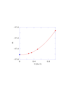
FIG. 1.: The energy for $N_{e}=10$ and $U=8$ on the $4\times 4$ lattice. The results for $\psi_{{\rm G}}$, $\psi^{(1)}$, $\psi^{(2)}$ and $\psi^{(3)}$ are shown. The diamond denotes the exact value.

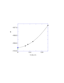
FIG. 2.: The energy for $N_{e}=82$ and $U=4$ on the $10\times 10$ lattice. The results for $\psi_{{\rm G}}$, $\psi^{(1)}$, $\psi^{(2)}$ and $\psi^{(3)}$ are shown. The square denotes the expectation value by CPMC and the triangle denotes that by QMC.

TABLE II.: Correlation functions for the $4\times 4$ Hubbard model with periodic boundary conditions in both directions. $N_{e}=10$, $U=4$ and $\psi_{0}$ is the normal free electron state.

	$\psi_{G}$	$\psi^{(2)}$	CPMC	Exact
$S(\pi,\pi)$	0.808	0.73	0.729	0.733
$C(\pi,\pi)$	0.460	0.52	0.508	0.506
$\Delta_{yy}(1)$	0.080	0.076		0.077
$\Delta_{yy}(2)$	0.007	0.006		0.006
$\Delta_{xy}(0)$	0.133	0.12		0.122
$\Delta_{xy}(1)$	-0.013	-0.015		-0.014
$s(0,0)$	0.525	0.53		0.533
$s(1,0)$	-0.098	-0.091		-0.0911
$c(0,0)$	0.33	0.33		0.326
$c(1,0)$	-0.047	-0.056		-0.0539

In Table II the correlation functions are defined by

$$s(i_{x},i_{y})=\langle(n_{0\uparrow}-n_{0\downarrow})(n_{i\uparrow}-n_{i\downarrow})\rangle~{}~{}{\rm for}~{}{\bf r}_{i}=(i_{x},i_{y}),$$ (31)

$$c(i_{x},i_{y})=\langle(n_{0}-\langle n_{0}\rangle)(n_{i}-\langle n_{i}\rangle)\rangle~{}~{}{\rm for}~{}{\bf r}_{i}=(i_{x},i_{y}),$$ (32)

where $n_{i}=n_{i\uparrow}+n_{i\downarrow}$. $S({\bf q})$ and $C({\bf q})$ are Fourier transforms of $s(i_{x},i_{y})$ and $c(i_{x},i_{y})$, respectively:

$$S({\bf q})=\sum_{i}{\rm exp}(i{\bf q}\cdot{\bf r}_{i})s({\bf r}_{i}),$$ (33)

$$C({\bf q})=\sum_{i}{\rm exp}(i{\bf q}\cdot{\bf r}_{i})c({\bf r}_{i}).$$ (34)

The superconducting correlation function $\Delta_{\alpha\beta}(\ell)$ is defined by

$$\Delta_{\alpha\beta}(\ell)=\langle\Delta^{{\dagger}}_{\alpha}(i+\ell\hat{x})\Delta_{\beta}(i)\rangle,$$ (35)

where $\Delta_{\alpha}(i)=c_{i\downarrow}c_{i+\alpha\uparrow}-c_{i\uparrow}c_{i+\alpha\downarrow}$ ($\alpha=\hat{x}$ or $\hat{y}$; $\hat{x}$ and $\hat{y}$ indicate an unit vector in x and y direction, respectively). The expectation values of correlation functions agree with the exact values considerably well. In these calculations $\psi^{(2)}$ satisfactorily reproduces the correlation functions as well as the ground state energy. In Table II, parameters are given by $g=0.30$, $\lambda=0.07$, $g^{\prime}=0.36$ and $\lambda^{\prime}=0.13$ (for $U=4$).

Now let us show an another example where we consider the $4\times 4$ lattice with 14 electrons for the periodic boundary condition in both directions. A famous sign problem occurs in this case for which the standard projector QMC method gives poor estimates of energy for large $U$. The quantum number of total momentum for $\psi^{\sigma}_{0}$ can take $(0,\pi)$ and $(\pi,0)$ as well as (0,0). Two kinds of initial trial states $\psi_{0}$ are examined; one is the Fermi sea with zero total momentum for both spin states and the other one has non-zero total momentum $(0,\pi)$ for each spin state. We incorporate the antiferromagnetic order into a trial wave function in the latter case since the energy gain is appreciable. In Table III we show our data. The extrapolated values are obtained as shown in Figs.3 and 4 where the solid curve and dotted curve indicate the energies obtained for SDW and normal initial states, respectively. Our calculations are supported by the property that the extrapolated values for different initial states coincides with each other within statistical errors. The energy obtained for $\psi^{(3)}$ is comparable with that by CPMC for large $U$ and extrapolated values are fairly close to exact values.

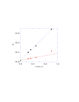
FIG. 3.: The energy as a function of $1/(m+1)$ for $N_{e}=14$ and $U=4$ on $4\times 4$. For the upper and lower curves an initial function $\psi_{0}$ is set to be the Fermi sea or SDW state, respectively. The diamond indicates the exact value.

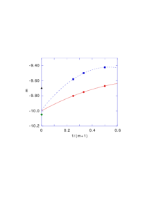
FIG. 4.: The energy as a function of $1/(m+1)$ for $N_{e}=14$ and $U=12$ on $4\times 4$. For the upper and lower curves an initial function $\psi_{0}$ is set to be the Fermi sea or SDW state, respectively. The diamond indicates the exact value and the triangle indicates CPMC result.

TABLE III.: Ground state energies for the $4\times 4$ Hubbard with $N_{e}=14$ for the periodic boundary conditions in both directions, where $U=4$ and $U=12$. $\psi_{0}$ is the non-interacting Fermi sea (normal) or SDW state (SDW) as indicated. The exact diagonalization results are from Ref.?.

$U$	$\psi_{0}$	$\psi^{(0)}$	$\psi^{(2)}$	$\psi^{(3)}$	Extrapolated	C PMC	Exact
4	normal	-14.435	-15.29	-15.40	-15.73	-15.73	-15.74
4	SDW	-15.34	-15.65	-15.67	-15.73		-15.74
12	normal	-7.80	-9.50	-9.58	-9.98	-9.696	-10.048
12	SDW		-9.75	-9.80	-10.0		-10.048

IV Results for the half-filled case

In this section the 2D square lattice with the half-filled band is investigated as a first step toward more general cases. The half-filled band systems have been studied numerically by the QMC simulation^? and VMC calculations.^?? In our calculations we impose the periodic boundary condition in one direction and antiperiodic condition in the other direction to have a unique ground state. Two sizes, $6\times 6$ and $8\times 8$, are investigated in this section.

The energy expectation values estimated by the off-diagonal wave function Monte Carlo method (OWMC) are shown as a function of $1/(m+1)$ for $6\times 6$ in Fig.5. The solid curves are drawn by the least squares method for three data points obtained by $\psi^{(1)}$, $\psi^{(2)}$ and $\psi^{(3)}$. The extrapolated values are used to obtain the total energy as a function of $U$ as shown in Fig.6 for $6\times 6$. In Fig.6 the energies for $\psi_{{\rm G}}=P_{{\rm G}}\psi_{0}$, $P_{\rm G}\psi_{{\rm SDW}}$, $\psi^{(2)}$ and extrapolated values are shown together. For the Gutzwiller function the energy is greatly lowered when the antiferromagnetic order is introduced. We obtain lower energies than those for $P_{G}\psi_{{\rm SDW}}$ by using the off-diagonal wave functions. In order to find optimum parameters we use the correlated measurements method^?? to find the most descendent direction in the parameter space. We shift parameters along that direction starting from a set of parameters. We show our parameters in Table IV. The extrapolations for $8\times 8$ as a function of $1/(m+1)$ are shown in Fig.7 where the upper and lower curves correspond to $U=8$ and $U=4$, respectively. The energy expectation values for $8\times 8$ are also shown in Fig.8 where the energies by $\psi_{{\rm G}}$, $P_{G}\psi_{{\rm SDW}}$, $\psi^{(2)}$ and extrapolation are compared to one another. The variational energy of $\psi^{(3)}$ is very close to that of $\psi^{(2)}$ and the extrapolated value. The results by the quantum Monte Carlo simulation by Hirsch are also shown as a reference. Although the QMC gives slightly higher energy for $U=8$, a good agreement between two calculations support our method as well as the QMC simulation. It is fortunate that the total energy for the intermediate value of $U$ is almost independent of the system size, which means that the extrapolated energies per site for $6\times 6$ and $8\times 8$ coincide with each other. Thus the energies in Figs.6 and 8 are expected to agree with the behavior of infinite systems.

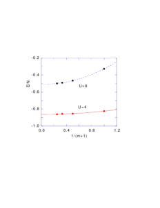
FIG. 5.: The energy as a function of $1/(m+1)$ for $6\times 6$ at half-filling. The upper and lower curves correspond to $U=8$ and $U=4$, respectively.

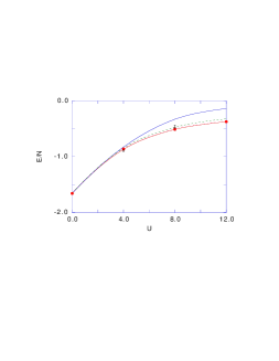
FIG. 6.: The energy as a function of $U$ for $6\times 6$ at half-filling. From the top the energies for $\psi_{{\rm G}}$, $P_{{\rm G}}\psi_{{\rm SDW}}$, $\psi^{(2)}$ and extrapolated values are shown. The QMC results for $8\times 8$ are shown by open circles as a reference.

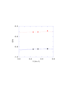
FIG. 7.: The energy as a function of $1/(m+1)$ for $8\times 8$ at half-filling. The upper and lower curves correspond to $U=8$ and $U=4$, respectively.

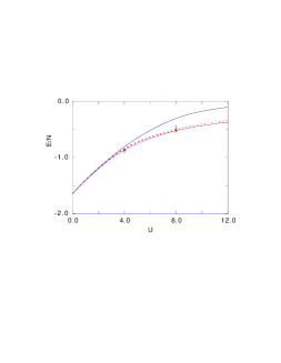
FIG. 8.: The energy as a function of $U$ for $8\times 8$ at half-filling. From the top the energies for $\psi_{{\rm G}}$, $P_{{\rm G}}\psi_{{\rm SDW}}$, $\psi^{(2)}$ and extrapolated values are shown. The QMC results are shown by open circles.

TABLE IV.: Variational parameters used in the simulation for $6\times 6$.

$U$	wave function	$g$	$\lambda$	$g^{\prime}$	$\lambda^{\prime}$	$g^{\prime\prime}$	$\lambda^{\prime\prime}$
4	$\psi_{{\rm G}}$	0.55	0.0	1.0	0.0	1.0	0.0
	$\psi^{(1)}$	0.18	0.118	1.0	0.0	1.0	0.0
	$\psi^{(2)}$	0.47	0.00064	0.44	0.123	1.0	0.0
	$\psi^{(3)}$	0.40	0.105	0.38	0.126	0.398	0.128
8	$\psi_{{\rm G}}$	0.24	0.0	1.0	0.0	1.0	0.0
	$\psi^{(1)}$	0.064	0.103	1.0	0.0	1.0	0.0
	$\psi^{(2)}$	0.17	0.00247	0.14	0.103	1.0	0.0
	$\psi^{(3)}$	0.18	0.159	0.128	0.197	0.142	0.096

The spin structure factor defined as

$$S({\bf q})=\frac{1}{N}\sum_{j\ell}{\rm exp}(i{\bf q}\cdot({\bf r}_{j}-{\bf r}_{\ell}))\langle(n_{j\uparrow}-n_{j\downarrow})(n_{\ell\uparrow}-n_{\ell\downarrow})\rangle,$$ (36)

can also be evaluated with our method, where $N$ denotes the total number of sites. We show $S({\bf q})$ calculated by $\psi^{(2)}$ and $\psi^{(3)}$ for $U=8$ in Figs.9 and 10, respectively, as a function of $q_{x}$ and $q_{y}$. The strong antiferromagnetic feature is shown in the figures with highly enhanced component at ${\bf q}=(\pi,\pi)$.

FIG. 9.: The spin structure factor for $\psi^{(2)}$. $U=8$ for $8\times 8$ where $q(x)=q_{x}/\pi$ and $q(y)=q_{y}/\pi$.

FIG. 10.: The spin structure factor for $\psi^{(3)}$. $U=8$ for $8\times 8$ where $q(x)=q_{x}/\pi$ and $q(y)=q_{y}/\pi$.

The sublattice magnetization $m$ has been calculated as a function of $U$ with the optimum variational parameters. The sublattice magnetization is defined as

$$m=\frac{1}{N}|\sum_{j}(-1)^{j}\langle n_{j\uparrow}-n_{j\downarrow}\rangle|$$ (37)

$m$ is plotted in Fig.11 as a function of $U$ where the calculated values obtained by $\psi^{(3)}$ (for $6\times 6$ and $8\times 8$), $P_{{\rm G}}\psi_{{\rm AF}}$^? are shown comparing with QMC method.^? Our results are substantially lower than the VMC predictions with the antiferromagnetically ordered state $P_{{\rm G}}\psi_{{\rm AF}}$ and show a good agreement with QMC results. The spin fluctuations appreciably reduce the sublattice magnetization but do not destroy the order in two dimensions.

V Summary

We have presented a new variational quantum Monte Carlo method for the Hubbard model. Our method is based on the property that we can systematically improve a variational wave function starting from the Gutzwiller wave function. It is remarkable that the variational energy is greatly lowered by the Gutzwiller and off-diagonal projection operators. For the $4\times 4$ lattice our results agree remarkably well with the exact values obtained by the exact diagonalization. Our calculations include the case where a sign problem occurs for the standard projector QMC. The results for $4\times 4$ and $10\times 10$ (in Table I) suggest that lower level off-diagonal functions show up as good a level of approximations as the constrained path QMC. The extrapolated values are favorably compared with exact results. For the 2D half-filled band system, we have calculated the exact energy as a function of $U$, which is lower than that by the antiferromagnetically ordered Gutzwiller function and mostly independent of the system size. There is a good agreement with the results by the QMC simulation concerning the energy and spin structure factor $S({\bf q})$. Thus we have demonstrated that the off-diagonal wave function Monte Carlo (OWMC) is useful to investigate the ground state for strongly correlated electrons.

In our simulation we spent most of time to search variational parameters optimizing the energy expectation values. We use the correlated measurements method to find a most descendent direction along which we shift the variational parameters starting from a set of initial parameters. Once the optimized parameters are determined, the expectation values are estimated with a large number of Monte Carlo steps.

In the process of OWMC we must evaluated $\langle c^{{\dagger}}_{i\sigma}c_{j\sigma}\rangle$ to estimate the kinetic energy, which is the second process costing a lot of time in the simulation. We feel that there is a room to improve our algorithm on this point.

Following a first step toward a development of the variational theory based on the off-diagonal wave functions performed in this paper, we are planning to consider some problems for correlated electrons. In particular, a possibility of the superconductivity for the non-half-filled band is considered to be an interesting one. An application to other models also deserves an investigation.

We thank Professor H. Aoki and Dr. K. Kuroki for useful comments and discussions. We express our sincere thanks to Professor P. Fulde for his suggestion about considering exp-$S$ type functions in the simulation. Our computations were supported by Research Information Processing System (RIPS) at the Agency of Industrial Science and Technology (AIST) in Tsukuba.

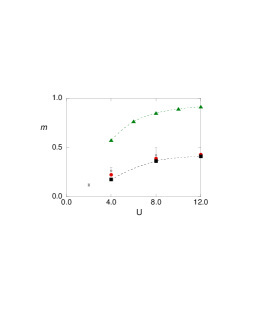
FIG. 11.: The sublattice magnetization as a function of $U$. The results by $\psi^{(3)}$ (solid circles for $6\times 6$ and squares for $8\times 8$), $P_{{\rm G}}\psi_{{\rm AF}}$ (triangles) and QMC (open circles).^?

References

- 1 N.F. Mott, Metal-Insulator transitions (Taylor and Francis Ltd., London, 1974).
- 2 P.W. Anderson, Science 235 (1987) 1196.
- 3 J.E. Hirsch, Phys. Rev. Lett. 54 (1985) 1317.
- 4 S.R. White, D.J. Scalapino, R.L. Sugar, E.Y. Loh, J.E. Gubernatis, and R.T. Scalettar, Phys. Rev. B40 (1989) 506.
- 5 D.J. Scalapino, in High Temperature Superconductivity - the Los Alamos Symposium - 1989 Proceedings, edited by K.S. Bedell, D. Coffey, D.E. Deltzer, D. Pines and J.R. Schrieffer (Addison-Wesley Publ. Comp., Redwood City, 1990) p.314.
- 6 T. Giamarchi and C. Lhuillier, Phys. Rev. B43 (1991) 12943.
- 7 T. Nakanishi, K. Yamaji and T. Yanagisawa, J. Phys. Soc. Jpn. 66 (1997) 294.
- 8 K. Kuroki and H. Aoki, Phys. Rev. B56 (1997) 14287.
- 9 K. Yamaji, T. Yanagisawa, T. Nakanishi and S. Koike, to be published in Physica C (1998).
- 10 K. Yamaji and Y. Shimoi, Physica C222 (1994) 349; K. Yamaji, Y. Shimoi and T. Yanagisawa, Physica C235-240 (1994) 2221.
- 11 T. Yanagisawa, Y. Shimoi and K. Yamaji, Phys. Rev. B52 (1995) 3860.
- 12 K. Kuroki, T. Kimura and H. Aoki, Phys. Rev.B22 (1996) 15641.
- 13 D. Ceperley, G.V. Chester and K.H. Kalos, Phys. Rev. B16 (1997) 3081.
- 14 H.Yokoyama and H.Shiba, J. Phys. Soc. Jpn. 56 (1987) 1490.
- 15 C. Gros, R. Joynt and T.M. Rice, Phys. Rev. B36 (1987) 381.
- 16 H. Ohtsuka, J. Phys. Soc. Jpn. 61 (1992) 1645.
- 17 T. Yanagisawa, T. Nakanishi, S. Koike and K. Yamaji, The Review of High Pressure Science and Technology 7 (1998) 154.
- 18 T. Yanagisawa, S. Koike and K. Yamaji, unpublished.
- 19 R. Blankenbecler, D.J. Scalapino and R.L. Sugar, Phys. Rev. D24 (1981) 2278.
- 20 M. Imada and Y. Hatsugai, J. Phys. Soc. Jpn. 58 (1989) 3752.
- 21 S. Zhang, J. Carlson and J.E. Gubernatis, Phys. Rev. B55 (1997) 7464.
- 22 N. Furukawa and M. Imada, J. Phys. Soc. Jpn. 61 (1992) 3331.
- 23 A. Parola et al., Physica C162 (1989) 771.
- 24 J.E. Hirsch, Phys. Rev. B31 (1985) 4403.
- 25 H. Yokoyama and H. Shiba, J. Phys. Soc. Jpn. B56 (1987) 3582.
- 26 C.J. Umrigar, K.G. Wilson, and J.W. Wilkins, Phys. Rev. Lett. 60 (1988) 1719.
- 27 K. Kobayashi and K. Iguchi, Phys. Rev. B47 (1993) 1775.