Abstract

We investigated the anomalous peak resistivity below the onset $T_{c}$ in underdoped YBCO, reminiscent of that observed in 1D wires of conventional superconductors. We performed measurements of the angular dependence of resistivity $\rho(\theta)$ in a magnetic field and the temperature dependence of resistivity $\rho(T)$, which exhibit a peak for $\textbf{B}\parallel$ ab-planes. This peak in $\rho(T)$ disappears for $\textbf{B}\parallel$ c-axis. The width of the corresponding maximum in $\rho(\theta)$ at $\theta=0^{o}$ ($\textbf{B}\parallel$ ab-planes) decreases with increasing c-axis component of the field ($B\sin\theta$). The maximum in $\rho(\theta)$ and $\rho(T)$ decreases with an increasing applied transport current. We analyzed the data using three different models of resistivity based on 2D resistor array, flux motion, and thermally activated phase-slips. Numerical calculations suggest that in a filamentary underdoped system, the phase-slip events could produce the anomalous resistivity close to $T_{c}$.

1 INTRODUCTION

Observation of a large resistive peak in the temperature dependence of resistivity $\rho(T)$ just below the onset $T_{c}$ has been reported in crystals of high $T_{c}$ superconductors (HTSC) like $(Nd,Pr)_{1.85}Ce_{0.15}CuO_{4-y}$ [1], YBCO(123) [2], and BSCCO(2212) [3]. In all these cases, the magnitude of the resistive peak is higher than the resistivity at the onset $T_{c}$. The peak shows an anomalous behavior in a magnetic field applied along the c-axis. Its magnitude decreases with an increasing field, and in high enough fields the peak is completely suppressed. The applied transport current has the same effect on the peak i.e the peak’s magnitude decreases with an increasing applied current.

These phenomena are of considerable interest because of their striking qualitative similarity to those observed in conventional superconductors (LTSC) like superconducting mesoscopic Al wires [4, 5], thin films of Al [6, 7], $(NbV)N$, NbV, VN, (NbTi)N [8], and disordered metallic glasses of $Zr_{60}Cu_{60}$ [9]. Mosqueira et al [2] reported the resistive anomalous peak in $\rho_{ab}(T)$ of YBCO crystals of $T_{c}(R=0)=89K$. This anomaly was eliminated by successive annealing of the sample in oxygen. This annealing also led to an increase of $T_{c}(R=0)$ up to 90.3 K (close to the optimal doping). The authors concluded that the peak could be related to very small $T_{c}$-inhomogeneities non-uniformly distributed in the crystal. They performed computer simulations of the temperature dependence of the anomalous resistivity using the model of two-dimensional electric circuit: an array of resistors whose resistivity depends on temperature. The non-uniformly distributed $T_{c}$-inhomogeneities were introduced by assuming that these resistors have different (higher or lower) $T_{c}$. The authors stated that the uniformly distributed $T_{c}$-inhomogeneities at large length scales broaden the resistive transition only, and do not produce a peak. Similar approach was introduced earlier by Vaglio et al [8] to explain the resistance-peak anomaly in non-homogeneous thin films of (NbV)N, NbN, VN, and (NbTi)N. They concluded that ”the current redistribution” caused by the sample’s inhomogeneity, is responsible for the observed phenomena.

Current redistribution effects in an inhomogeneous sample were also considered by Nordstrom and Rapp [9] in their interpretation of the resistive peak anomaly in superconducting amorphous thick films of $Zr_{60}Cu_{40}$. Kwong et al [6] observed an anomalous peak in the resistive transition of a 2D 25 nm thick aluminium film containing regions of different but comparable, transition temperatures. Disordered regions of lower $T_{c}$ were produced by the reactive-ion etching process. Their observation seems to support earlier interpretations based on $T_{c}$-inhomogeneities and current redistribution effects. The authors stated, however, that the anomaly could originate from a discontinuity of the superconducting potential at the normal-superconducting metal (N-S) interface, and for superconducting electrodes placed sufficiently close to the interface, this potential exceeds the normal-state value. Spahn and Keck [7] found that the anomaly appears in 2D Al films with thickness between 13 and 40 nm. They argued that this effect could be caused by an interaction between the superconducting fluctuations and the conduction electrons.

Extensive studies of the resistive anomaly were also performed on 1D Al strips with a width less than the coherence length and the magnetic penetration depth, by Santhanam et al [4] and Moshchalkov et al [5]. Santhanam et al argued that the Al wire could be treated (at temperatures close to $T_{c}$) as a coherent region comprising normal (N) and superconducting (S) phases. The resulting N-S interface gives rise to a quasiparticle charge imbalance induced by the bias current, and consequently to the observed changes in resistivity. Moshchalkov et al performed quantitative analysis of the anomaly using Langer-Ambegaokar (LA) [10] and McCumber-Halperin (MH) [11] models of the thermally activated phase-slips of the superconducting order parameter. LA-MH models were adopted with the modification which assumes that in quasi-1D superconducting wires the normal current and the supercurrent can only flow in series, and the total resistance is the sum of the normal resistance $R_{N}$ and the phase-slip resistance $R_{S}$. Good quantitative agreement between the experimental data and the calculated resistance R(T) was obtained.

Crusellas et al [1] and Han et al [3] proposed that the anomaly in $\rho_{ab}(T)$ of $(Pr,Nd)_{1.85}Ce_{0.15}CuO_{4-y}$ and BSCCO(2212) crystals is the manifestation of a quasireentrant behavior, which results from the intrinsic granularity. Han et al rejected the explanation based on non-uniformly distributed $T_{c}$-inhomogeneities (Ref.[2]), because of the observation of an anomalous peak in the I-V characteristics, which were measured at different magnetic fields. However, Crusellas et al [1] stated that the anomaly is strongly influenced by the distribution of defects, after it was observed that high temperature annealing reduces the size of the resistive anomaly in $(Pr,Nd)_{1.85}Ce_{0.15}CuO_{4-y}$ crystals.

Briefly, the interpretation of the anomalous resistive peaks in HTSC concentrates on two possible sources of this effect: non-uniformly distributed $T_{c}$-inhomogeneities and intrinsic granularity. The explanation of the anomalous resistivity in LTSC films took into account the effects of $T_{c}$-inhomogeneities (and related current redistribution), N-S interfaces, and the interaction between superconducting fluctuations and the conduction electrons. It was also suggested that the anomaly in 1D LTSC (Al) strips (wires) originates from the presence of N-S interfaces and/or thermally activated phase-slips of the order parameter.

These various interpretations are the source of a number of unanswered questions:

1. According to Browning et al [12] in YBCO single crystals of $T_{c}$=93 K and transition width of $\Delta T_{c}$=0.2 K, large variation in the oxygen content $7-\delta$ can occur across the sample as revealed by high resolution scanning x-ray diffractometry (which was performed using $10\mu m$ wide x-ray beam). $7-\delta$ in these crystals ranges between 6.80 and 7.00, which corresponds to a change of $T_{c}$ by about 10 K. In spite of these non-uniform $T_{c}$-inhomogeneities, the crystals have small resistivities ($\rho\simeq 40\mu\Omega cm$ at 100 K) and do not show any resistive peak anomalies at the onset $T_{c}$ in $\rho(T)$. These results throw doubt on whether the 2D resistive model alone (as proposed in Ref.[2] for YBCO) can explain the observed anomalies.

2. The resistive anomalies observed in LTSC films and wires (strips) are similar and their interpretation suggest the link between the presence of inhomogeneities ($T_{c}$-inhomogeneities, N-S interfaces) and the superconducting fluctuations, including phase-slips of the order parameter. Could this explanation be also applied to HTSC?

3. Moshchalkov et al [5]introduced the phase slip resistivity ( according to the 1D LA-MH model [10, 11]) combined with the normal state resistivity in order to explain the anomalous resistive peak in 1D aluminum wires. Experiments by Browning et al [see (1)] suggest filamentary phase separation and filamentary flow of the current in some YBCO crystals with sharp superconducting transitions, which do not show resistive anomalies. Does this mean using the analogy to LTSC that the presence of non-uniformly distributed inhomogeneities in HTSC is the necessary but not sufficient condition to observe the resistive anomaly? What is the other condition? Could this be a 1D current flow in an inhomogeneous system?

4. What is the contribution of the magnetic flux motion (pinning) to the observed resistive anomalies in HTSC?

In order to answer these questions new experiments are needed. We decided to perform measurements of the angular dependence of resistivity in a magnetic field. This decision was stimulated by the experiments done on $Pr_{1.85}Ce_{0.15}Cu_{4-y}$ crystals [1], in which the resistive anomaly was investigated for two different directions of the applied magnetic field, namely along the c-axis and along the ab-planes. The effect of the magnetic field on the anomaly was completely different for these two orientations. Taking into account the fact that the presence of the non-uniform $T_{c}$-inhomogeneities is the necessary but not sufficient condition to observe the resistive anomalies, we investigated the temperature dependence of resistivity on a large number of YBCO samples. We decided to study YBCO thin films, both optimally doped and underdoped, because they are readily accessible from different research groups and can be deposited on various substrates using several different deposition techniques. The bridges for the resistive measurements can be made relatively easily on thin films using standard photolithographic techniques. The resistive peak anomaly and the reduction of its magnitude with an increasing magnetic field and an increasing applied current, were observed in an underdoped film after investigation of fifteen YBCO films of $T_{c}$ ranging between 79 and 90.5 K. This film was then used to perform detailed measurements of the angular dependence of resistivity in a magnetic field. The resulting experimental data were analyzed using three different models: two dimensional resistor model, magnetic flux motion model, and the LA-MH thermally activated phase -slip theory.

2 EXPERIMENTAL PROCEDURE

2.1 Sample Preparation

C-axis oriented YBCO thin films were prepared using off-axis rf magnetron sputtering and laser ablation from stoichiometric $YBa_{2}Cu_{3}O_{7-\delta}$ targets of 99.999% purity. Films were deposited on three different types of substrates: $SrTiO_{3}$, $LaAlO_{3}$, and sapphire (with $CeO_{2}$ buffer layer).

We investigated fifteen YBCO thin films (both underdoped and close to the optimal doping) of various zero-resistance transition temperatures (between 79 and 90.5K) and thicknesses (between 100 and 600nm). YBCO films were patterned, using conventional photolithography and wet etching technique, into a form of a $30-60\mu m$ wide and 6.4 mm long strips with six measurement probes. Large area silver contacts were deposited on the film by rf magnetron sputtering in order to minimize Joule heating. Copper leads were attached to silver contacts using mechanically pressed indium. The distance between voltage probes was 0.4 mm.

The anomalous resistivity was observed in an underdoped YBCO thin film. This film (140 nm thick), was deposited on a (1000) oriented sapphire substrate (with $CeO_{2}$ buffer layer) using laser ablation technique. The sample exhibits a vanishing zero-field resistivity at $T_{c}=81.7K$ and has a room temperature resistivity $\rho_{300K}=34.2\mu\Omega cm$ ($\frac{\rho_{300K}}{\rho_{100K}}=2.4$).

X-ray diffraction (XRD) data of this film showed the pattern of a characteristic stoichiometric c-axis oriented YBCO film. The data did not reveal any impurity phases. The XRD data gave a c-axis lattice spacing of 11.70 Å, which corresponds to an oxygen content of about 6.8 and $T_{c}(R=0)$ of about 80 K [13].

2.2 Measurement Procedure

The investigation of the resistive anomalies was based on the following measurements: (a) the measurement of the temperature dependence of resistivity $\rho(T)$ between room temperature and $T_{c}(R=0)$ in zero magnetic field; (b) the measurement of the temperature dependence of resistivity $\rho(T)$ between the onset $T_{c}$ and $T_{c}(R=0)$ in an external magnetic field applied either parallel or perpendicular to the ab-planes; (c) the measurement of the angular dependence of resistivity $\rho(\theta)$ as a function of the angle $\theta$ between the ab-planes and the direction of the fixed applied magnetic field at fixed temperatures between the onset $T_{c}$ and $T_{c}(R=0)$; (d) the measurement of $\rho(\theta)$ as a function of the magnitude of the magnetic field B and the applied transport current density J. The angular measurements were performed by rotating a copper sample holder about its vertical axis in a horizontal magnetic field up to 1 Tesla, using a combination of a step-motor and backlash-free gear reducer. The angle was accurately monitored by an 8000-line optical encoder attached to the sample, whose angular resolution was $0.045^{o}$. The film was mounted with the c-axis perpendicular to the sample holder’s vertical axis of rotation, which allowed one to change the magnetic field direction in a plane parallel to the c-axis.

Resistivity was measured using the standard dc four-probe method. The current was applied to the sample in the form of short pulses (of duration less than 200 ms) in order to reduce Joule heating. A dc current reversal was used to eliminate the thermal emf in the leads. The voltage was measured using a Keithley 2182 Nanovoltmeter in tandem with a Keithley 236 Current Source, with the nanovoltmeter working as the triggering unit. The nanovoltmeter was operated in a mode (known as Delta mode) which allows the measurement and calculation of the voltage from two voltage measurements for two opposite directions of the current. Temperature was monitored by a carbon-glass resistance thermometer and an inductanceless heater and was controlled to better than $\pm 10mK$ for each single angular sweep in a magnetic field. This was achieved by rotating the sample very slowly in the magnetic field in order to reduce variations in the emf in the heater which could disturb the temperature reading. The term ”resistivity” is used in this paper to denote the quantity $E/J$ (where E is the electric field and J is the transport current density), and it does not imply an ohmic response.

All measurements were carried out with the transport current J parallel to the ab-planes for two different orientations of the magnetic field with respect to the current. For the first one, the field was rotated in a plane perpendicular to the current direction while for the other one the field was rotated in a plane parallel to the current and the c-axis directions [see Fig.1(a)]. All measurements were done in a field cooling (FC) regime, with the magnetic field applied to the sample at a temperature above the onset $T_{c}$, followed by a slow cooling down to the required temperature of measurement.

3 EXPERIMENTAL RESULTS

3.1 Temperature dependence of resistivity

The temperature dependence of resistivity $\rho$ was measured over a temperature range of 78-300 K in a zero magnetic field. For a temperature range (78-90 K) close to $T_{c}$, $\rho$ was recorded for different orientations of the magnetic field with respect to the direction of the current density J. Fig.1(a) shows two possible orientations of the magnetic field B with respect to J and the ab-plane of the film. The figure on the left illustrates the case in which the field B was rotated in a plane parallel to the direction of J while the one on the right represents the case in which B was rotated in a plane perpendicular to J. For both orientations B was rotated in a plane parallel to the c-axis. The first configuration is denoted as $\textbf{B}\parallel\textbf{J}$ and the second one as $\textbf{B}\perp\textbf{J}$. Fig.1(b) shows the temperature dependence of resistivity $\rho(T)$ for a temperature range of 79-88 K measured in a zero field and in 0.68 T. The measurements of $\rho(T)$ in the field were carried out for the following orientations of B with respect to J: $\textbf{B}\parallel\textbf{J}$ and $\textbf{B}\perp\textbf{J}$ with B parallel to the ab-plane ($\theta=0^{o}$), and for $\textbf{B}\perp\textbf{J}$ with B parallel to the c-axis ($\theta=90^{o}$). The onset transition temperature (onset $T_{c}$) is defined as the temperature above which the resistivity does not respond to the change in both magnitude and direction of the magnetic field [see Fig.1(b)]. $\rho(T)$ below the onset $T_{c}$ could be divided into three regions. Each region is identified according to the response of $\rho(T)$ to the change in the direction of the magnetic field from the ab-planes ($\theta=0^{o}$) to the c-axis ($\theta=90^{o}$). Region II represents a temperature range between 82.8 K and 83.5 K over which $\rho(T)$ exhibits a peak (of magnitude larger than that of $\rho(T)$ at the onset $T_{c}$) in a zero magnetic field, and for $\textbf{B}\parallel$ ab-planes with $\textbf{B}\parallel\textbf{J}$ and $\textbf{B}\perp\textbf{J}$ orientations. Note a clear separation between the peak and the onset $T_{c}$. In this region, behavior of $\rho(T)$ changes dramatically upon rotating the field from the ab-planes to the c-axis. In regions I and III, $\rho(T)$ was observed to increase when B is parallel to the c-axis, while in region II (the peak region) $\rho(T)$ is completely suppressed by the magnetic field $\textbf{B}\parallel$ c-axis. For $\textbf{B}\parallel$ ab-planes, $\rho(T)$ in regions I and III is independent of the magnitude of B and the angle between B and J. However, in region II, $\rho(T)$ is independent of the magnitude of B only for $\textbf{B}\parallel\textbf{J}$ orientation. In this region, $\rho(T)$ was found to decrease with an increasing applied current density J. The temperature dependence of resistivity for $\textbf{B}\parallel c$-axis was measured in different magnetic fields. For fields above 0.1 T, the peak in region II is completely suppressed. The resistivity between the onset $T_{c}$ and the room temperature exhibits a linear temperature dependence.

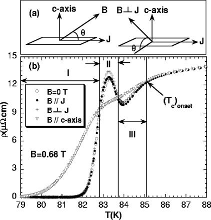
Figure 1: (a) Two configurations of B with respect J that were used during the measurements of the angular dependence of resistivity $\rho(\theta)$ in a magnetic field: B is rotated in a plane parallel to both J and the c-axis (left side), or B is rotated in a plane parallel to the c-axis but perpendicular to J (right side). (b) Temperature dependence of resistivity for YBCO thin film measured in a zero and 0.68 T fields at different orientations. Regions I and III denote the temperature ranges over which $\rho(T)$ is independent of the magnitude of B and the angle between B and J for $\textbf{B}\parallel$ ab-planes. In these regions $\rho(\theta)$ displays a minimum at $\theta=0^{o}$ (B parallel to the ab-planes) [see Fig.2(a) and (c)]. Region II represents the temperature range over which $\rho(T)$ exhibits a peak (of magnitude larger than $\rho(T)$ at the onset $T_{c}$), for B=0 and for both $\textbf{B}\parallel\textbf{J}$ ($\theta=0^{o}$) and $\textbf{B}\perp\textbf{J}$ ($\theta=0^{o}$) orientations. Rotating the field from the ab-planes ($\theta=0^{o}$) towards the c-axis ($\theta=90^{o}$), leads to an increase in $\rho(T)$ in regions I and III and to a suppression of the peak in region II.

3.2 Angular dependence of resistivity: Effect of temperature and magnetic field

The angular dependence of resistivity $\rho(\theta)$ was measured in a constant magnetic field at different temperatures in regions I, II, and III, for both $\textbf{B}\parallel\textbf{J}$ and $\textbf{B}\perp\textbf{J}$ orientations for the angular range from $-20^{o}$ to $+20^{o}$. The measurements revealed minima in $\rho(\theta)$ at $\theta=0^{o}$ in region I and III, and a maximum in region II (see Fig.2). Fig.2(a) shows $\rho(\theta)$ in region I as a function of temperature between 82.42 K and 82.82 K in a magnetic field of 0.68 T. At a temperature of approximately 82.82 K, which corresponds to the border line between region I and II in Fig.1(b), there is a crossover from a minimum to a peak in $\rho(\theta)$. This peak grows with an increasing temperature reaching a maximum value at 83.23 K (see Fig.2(b)).

Fig.2f.eps

Figure 2: $\rho(\theta)$ measured in 0.68 T for a temperature range between 82.52 K and 83.83 K spanning the three regions I, II, and III. Note the change in $\rho(\theta)$ at $\theta=0^{o}$ from a minimum in region I (a) to a maximum in region II (b) and then back to a minimum in region III (c). In regions I and III, identical behavior of $\rho(\theta)$ has been observed for $\textbf{B}\parallel\textbf{J}$ and $\textbf{B}\perp\textbf{J}$ orientations, whereas in region II the magnitude of $\rho(\theta)$ depends on those orientations.

The second crossover from a maximum to minimum can be seen at 83.50 K, which corresponds to the border line between regions II and III in Fig.1(b). We have measured $\rho(\theta)$ for both $\textbf{B}\perp\textbf{J}$ and $\textbf{B}\parallel\textbf{J}$ in all three regions. While in regions I and III the minimum in $\rho(\theta)$ is independent of the orientation of B with respect to J (i.e for $\textbf{B}\perp\textbf{J}$ and $\textbf{B}\parallel\textbf{J}$), in region II the magnitude of the peak depends on these orientations and $\rho(\theta)_{B\perp J}>\rho(\theta)_{B\parallel J}$.

The measurements of $\rho(\theta)$ over an angular range between $-30^{o}$ and $210^{o}$ revealed sharp maxima for $\textbf{B}\parallel$ ab-planes ($\theta=0^{o}$ and $\theta=180^{o}$) and a smaller broad maximum for $\textbf{B}\parallel$ c-axis ($\theta=90^{o}$) (see Fig.3). $\rho(\theta)$ at $\theta=0^{o}$ and $\theta=180^{o}$ is about 30% larger than that for $\theta=90^{o}$. Moreover $\rho(\theta)$ has minima at $\theta=35^{o}$ an $\theta=145^{o}$ for all fields.

Fig.3f.eps

Figure 3: $\rho(\theta)$ measured in 0.68 T at 83.23 K for an angular range $-30^{o}<\theta<210^{o}$. Note the peaks at $\theta=0^{o}$ and $\theta=180^{o}$ ($\textbf{B}\parallel$ ab-planes) which are approximately 30% higher than the maximum at $\theta=90^{o}$ ($\textbf{B}\parallel$ c-axis).

Fig.4.eps

Figure 4: (a) Angular dependence of resistivity measured at a temperature of 81.43 K (region I) in different fields for B close to the ab-planes. The data reveal a minimum in $\rho(\theta)$ at $\theta=0^{o}$ (B parallel to the ab-planes). The width of the minimum decreases with an in increasing field. An identical behavior has been observed for both $\textbf{B}\perp\textbf{J}$ and $\textbf{B}\parallel\textbf{J}$ orientations.

The angular dependence of resistivity $\rho(\theta)$ was also measured at a constant temperature in different magnetic field in regions I, II, and III, for both $\textbf{B}\parallel\textbf{J}$ and $\textbf{B}\perp\textbf{J}$ orientations and for the angular range between $-20^{o}$ and $+20^{o}$. Fig.4 shows the angular dependence of resistivity, at a temperature of 81.43 K (region I), measured in different magnetic fields for both $\textbf{B}\parallel\textbf{J}$ and $\textbf{B}\perp\textbf{J}$ orientations. The data for these two orientations are identical which implies that $\rho(\theta)$ is independent of the angle between B and J. $\rho(\theta)$ at $\theta=0^{o}$ is almost independent of the magnitude of B. The width of this minimum [defined as half width at half minimum (HWHM)] decreases from HWHM=$2.3^{o}$ in a field of 0.17 T down to HWHM=$2.0^{o}$ in 0.86 T. The depth of the minimum increases with an increasing field. The results of the measurements of $\rho(\theta)$ in region III is identical in all aspects to those obtained in region I.

Fig.5 presents $\rho(\theta)$ measured at a temperature of 83.13 K (in region II) in different magnetic fields for both $\textbf{B}\perp\textbf{J}$ and $\textbf{B}\parallel\textbf{J}$ orientations. The width of the peak in $\rho(\theta)$ decreases with an increasing B for both $\textbf{B}\perp\textbf{J}$ and $\textbf{B}\parallel\textbf{J}$ orientations. The magnitude of the peak in $\rho(\theta)$ for $\textbf{B}\parallel\textbf{J}$ is almost independent of the magnitude of B, however it increases with B for $\textbf{B}\perp\textbf{J}$. A decrease of the peak’s width with an increasing magnetic field means that within a certain angular range ($\mid\theta\mid>1.5^{o}$ for $\textbf{B}\perp\textbf{J}$ and $\mid\theta\mid>0.3^{o}$ for $\textbf{B}\parallel\textbf{J}$), $\rho(\theta)$ decreases with an increasing field.

Fig.5.eps

Figure 5: Angular dependence of resistivity $\rho(\theta)$ for $-5^{o}<\theta<5^{o}$, measured in different applied magnetic fields at a fixed temperature of 83.13 K (region II). (a) $\rho(\theta)$ for $\textbf{B}\perp\textbf{J}$ orientation, where $\rho(\theta)$ increases with an increasing B for $\theta<1^{o}$ but decreases with an increasing B for $\theta>1^{o}$. (b) $\rho(\theta)$ for $\textbf{B}\parallel\textbf{J}$ orientation; $\rho$ at $\theta=0^{o}$ is almost independent of B. Note that $\rho(\theta)$ decreases with an increasing B for $\theta>0.5^{o}$.

3.3 Angular dependence of resistivity: Effect of the applied current

The angular dependence of resistivity was measured also as a function of the applied current density at a constant temperature and magnetic field. Fig.6 presents the measurements of $\rho(\theta)$ in region II for a wide range of applied current density J, from 0.9 to 69.4 $kA/cm^{2}$, in a field of 0.68 T and at a temperature of 83.03 K. For angles $\mid\theta\mid>2^{o}$, $\rho(\theta)$ increases non-linearly with an increasing J, but for small angles $\mid\theta\mid<2^{o}$ it decreases with an increasing J. In the angular region for $\mid\theta\mid<1^{o}$, starting at small current density ($\textbf{J}\leq 11.6kA/cm^{2}$), the peak height initially decreases with an increasing current, but for J larger than $23.1kA/cm^{2}$, a minimum in $\rho(\theta)$ develops. The dependence of $\rho(\theta)$ on J is essentially the same for both $\textbf{B}\parallel\textbf{J}$ and $\textbf{B}\perp\textbf{J}$ orientations.

Fig.6.eps

Figure 6: Angular dependence of resistivity $\rho(\theta)$ measured as a function of applied current density J for a field of 0.68 T and a temperature of 83.03 K (region II) . For angles $\mid\theta\mid>2^{o}$ , $\rho(\theta)$ increases with an increasing J, but for small angles $\mid\theta\mid<2^{o}$ the opposite happens, where a minimum starts to develop with its width increasing with an increasing applied current.

Fig.7 shows $\rho(\theta)$ measured in region I for a wide range of J in a field of 0.68 T and at a temperature of 81.83 K. Effect of the current on the minimum is different from that observed in region II. The minimum at $\theta=0^{o}$ decreases with an increasing J. The dependence of $\rho(\theta)$ on J is identical for both $\textbf{B}\parallel\textbf{J}$ and $\textbf{B}\perp\textbf{J}$ orientations. Similar dependence of $\rho(\theta)$ on J was observed over the temperature range in region III.

Fig.7.eps

Figure 7: (a) Angular dependence of resistivity $\rho(\theta)$ measured as a function of an applied current density J in a field of 0.68 T and at a temperature of 81.83 K (region I). The sharpness of the minimum at $\theta=0^{o}$ decreases gradually with an increasing J. (b) Expanded view of $\rho(\theta)$ measured at $J=57.9kA/cm^{2}$.

4 DISCUSSION

The experimental data for $\rho(T,B)$ obtained for the underdoped YBCO film are qualitatively similar to those observed before in HTSC [1, 2, 3]. The anomalous resistive peak is located at a temperature approximately 1.8K lower than the onset $T_{c}$. The peak disappears when a magnetic field is applied along the c-axis of the film. Also the magnitude of the peak decreases and its position shifts to lower temperatures with an increasing applied transport current. Our measurements of the angular dependence of resistivity in a magnetic field provided very valuable additional information, which allows us to understand better the physics of the anomalous resistivity. The measurements of $\rho(\theta)$ in a magnetic field as a function of temperature revealed sharp minima in resistivity at $\theta=0^{o}$ (B parallel to the ab-planes) at temperatures below and above the resistive peak in $\rho(T)$, and a sharp maximum at $\theta=0^{o}$ at the peak’s temperature (see Fig.2).

The data for $\rho(T)$ and $\rho(\theta)$ were used to distinguish between different interpretations of the resistive anomaly. We considered two-dimensional resistor model, magnetic flux motion, and thermally activated phase-slips.

4.1 Two-dimensional resistor model

In an inhomogeneous superconductor different parts of the film or the crystal can have slightly different transition temperatures. In this case the superconductor may be modelled as an electrical circuit- array of different resistors. The anomalous peak in $\rho(T)$ is produced by solving numerically, through the standard matrix method, the electrical circuit equations. This model was used to analyze the data, taken in a zero magnetic field, for anomalous resistivity in $\rho_{ab}(T)$ of YBCO crystal by Mosqueira et al [2], and in $\rho(T)$ of Nb-based LTSC films by Vaglio et al [8]. The calculated $\rho(T)$ agrees with the experimental data.

Mosqueira et al [2] also attempted to explain the suppression of the anomalous peak by a magnetic field in YBCO crystals using the resistor model. They argued that the reduction of the peak and its shift to low temperature is caused by the broadening of the superconducting transition $\Delta T_{c}(B^{*})$ in a magnetic field $B^{*}$ (and not just by the shift in $T_{c}$). The peak disappears when the superconducting transition broadens by about 2K in a field of 0.3T. According to the resistive model, the broadening required for the peak to be eliminated from $\rho(T)$ should be material-independent provided that the ratio $\Delta\rho/\rho_{B}=(\rho_{P}-\rho_{B})/\rho_{B}$ (where $\rho_{P}$ is the peak’s resistivity and $\rho_{B}$ is the resistivity measured in a magnetic field B at the peak’s temperature in the absence of the peak) does not change. The experimental data in Refs [1, 2, 3, 4] show that this is not the case. Table 1 lists the data for $\Delta\rho/\rho_{B}$, $\Delta T_{c}(B^{*})$, and the magnetic field $B^{*}$ at which the peak disappears, for different superconducting materials.

Table 1: $\Delta\rho/\rho_{B}$, $\Delta T_{c}(B^{*})$, and the magnetic field $B^{*}$ at which the peak disappears, for different superconductors.

Material	$\Delta\rho/\rho_{B}$	$B^{*}(T)$	$\Delta T_{c}(B^{*})(K)$	Ref
YBCO crystal	0.29	0.3	2	[2]
YBCO film	0.44	0.08	0.5	this work
BSCCO crystal	1.56	0.01	$\sim 2$	[3]
NdCeCuO crystal	0.28	0.1	$\sim 4$	[1]
PrCeCuO crystal	0.16	0.7	$<0.5$	[1]
Al wires	0.17-0.56	0.001	0	[4]

These data reveal that the disappearance of the peak from $\rho(T)$ in a magnetic field is not related to the broadening $\Delta T_{c}(B^{*})$ of the superconducting transition. Our data obtained on YBCO film (see Table 1) support this conclusion.

4.2 Flux-motion

In order to find the contribution of the magnetic flux motion to the observed resistive anomaly, we performed the measurements of $\rho(T)$ and $\rho(\theta)$ for two different orientations of the current relative to the magnetic field i.e for $\textbf{B}\perp\textbf{J}$ and $\textbf{B}\parallel\textbf{J}$ orientations (see Fig.1). The magnitude of the peak in $\rho(T)$ (region II in Fig.1) increases when the field is parallel to the ab-planes and perpendicular to the current i.e for $\textbf{B}\perp\textbf{J}$ (compared to the case for $\textbf{B}\parallel\textbf{J}$). This situation corresponds to the maximum Lorenz force acting on the flux lines along the ab-planes. The angular dependence of $\rho$ in a magnetic field (Fig.2) reveals a maximum in region II, but sharp minima at temperatures below and above the peak (regions I and III in Fig.1). A very sharp minimum in $\rho(\theta)$ at $\theta=0^{o}$ ($\textbf{B}\parallel$ ab-planes) was seen previously in a YBCO single crystal by Kwok et al [14] and interpreted as due to the lock-in transition of the flux lines trapped between the planes. For a system of weakly coupled $CuO_{2}$ layers one expects a maximum resistive dissipation for $\textbf{B}\parallel$ c-axis and a minimum for $\textbf{B}\parallel$ ab-planes. An increase in $\rho(\theta)$ when the field is rotated from the ab-planes to the c-axis is normally attributed to the intrinsic anisotropy of the material. We found that the minima in $\rho(\theta)$ at $\theta=0^{o}$ (regions I and III) are independent of the orientation of the current relative to B (see Fig.4), suggesting very strong flux lock-in mechanism when B is parallel to the ab-planes. For $\theta>0^{o}$ resistivity could arise via the nucleation and motion of kinks along the vortex lines [14]. In this case, one could also describe the tilted vortex line as the combination of Josephson strings aligned along the ab-planes and mobile pancakes (vortex segments along the c-axis). If the coupling between the pancake vortices is weak, the Lorenz force acting on these vortices and consequently their motion, should be independent of the direction of the transport current in the ab-planes. The measurement of the minimum in $\rho(\theta)$ also revealed an increase of the resistivity with an increasing transport current in the ab-planes (Fig.7), which is independent of the orientation of the current relative to B. This result suggests that the motion of the pancake-vortices in the ab-planes is responsible for the observed increase of $\rho(\theta)$ for $\theta>0^{o}$ in regions I and III. The maximum in $\rho(\theta)$ at $\theta=0^{o}$ at temperatures corresponding to region II in $\rho(T)$ (Fig.5) depends on the orientation of the current relative to B. For $\textbf{B}\perp\textbf{J}$ orientation, the maximum is higher than that measured for $\textbf{B}\parallel\textbf{J}$ orientation. This behavior is different from that observed in regions I and III and therefore it provides additional argument that the peak in $\rho(T)$ can not be explained by the 2D-resistor model alone. It also suggests that the unknown dissipation in region II weakens flux lock-in between the planes. Subtracting the maximum in $\rho(\theta)$ at $\theta=0^{o}$ for $\textbf{B}\parallel\textbf{J}$ from that measured for $\textbf{B}\perp\textbf{J}$ (see Fig.8) gives $\rho(\theta)$ with a minimum similar to those observed in regions I and III, which are caused by flux motion.

The measurement of the maxima in $\rho(\theta)$ at $\theta=0^{o}$ as a function of magnetic field for $\textbf{B}\parallel\textbf{J}$ and $\textbf{B}\perp\textbf{J}$ orientations shows that the maxima become sharper (i.e their width decreases) with an increasing magnetic field. For both $\textbf{B}\parallel\textbf{J}$ and $\textbf{B}\perp\textbf{J}$ orientations, and for $\theta>1.5^{o}$, the resistivity at a fixed $\theta$ decreases with an increasing field (Fig.5). On the other hand, the maximum in $\rho(\theta)$ at $\theta=0^{o}$ also decreases with an increasing transport current (Fig.6). This reduction in resistivity can not be explained by the flux motion. Chaparala et al [15] observed a small maximum in $\rho(\theta)$, when the magnetic field was oriented parallel to the ab-planes in Tl (2212, 1223) and Bi(2212) crystals. The authors did not present any data for the corresponding temperature dependence of resistivity. The maximum in resistivity was attributed to the formation and motion of the c-axis-oriented vortex-antivortex segments of the flux lines parallel to the ab-planes. They assumed that the maximum is created as a result of the interplay between the density $n_{s}$ and the velocity $v_{s}$ of the vortex-antivortex segments. The resistive potential difference V is proportional to the product of these quantities. According to the experimental observation $V\propto(n_{s}v_{s})_{\theta=0^{o}}$ is larger than $V\propto(n_{s}v_{s})_{\theta>0^{o}}$. Chaparala et al [15] argued that at $\theta=0^{o}$, in spite of the small density of the vortices, $n_{s}v_{s}$ is large because of the high velocity of the newly created vortex-antivortex pairs. At $\theta>0^{o}$, $n_{s}$ is large but $v_{s}$ is small, so $(n_{s}v_{s})_{\theta=0^{o}}>(n_{s}v_{s})_{\theta>0^{o}}$. According to this interpretation, increasing the applied transport current should increase the Lorenz force on these pairs and consequently increase their velocity. This leads to an increase in the resistive dissipation and to the growth of the maximum in $\rho(\theta)$ at $\theta=0^{o}$ with an increasing current. Our data revealed a reduction of the maximum in $\rho(\theta)$ at $\theta=0^{o}$ with an increasing current (see Fig.6), which eliminates the vortex-antivortex model as a possible explanation of the resistive anomaly. The absolute values of the resistivity in the peak observed on $\rho(T)$ curve is higher than the resistivity at the onset $T_{c}$ (85 K), defined as the temperature above which the resistivity is independent of the magnitude and direction of the applied magnetic field (see Fig.1). The resistive dissipation due to a vortex motion can reduce the critical current density to zero, reaching the normal state resistivity, but it can not exceed this value.

Fig.5f.eps

Figure 8: (a) Comparison between $\rho(\theta)$ measured for $\textbf{B}\perp\textbf{J}$ and $\textbf{B}\parallel\textbf{J}$ orientations in 0.68T at 83.13K. (b) The difference $\Delta\rho(\theta)$ between the peaks in $\rho(\theta)$ for $\textbf{B}\perp\textbf{J}$ and $\textbf{B}\parallel\textbf{J}$ orientations measured in 0.34 T and 0.68 T.

4.3 Phase-slip model

Discussion of the resistive-peak anomaly in the previous sections indicates that 2D-resistor and flux motion models alone can not fully account for the origin of this phenomenon. Regarding LTSC, Moshchalkov et al [5] argued that the resistive anomaly, seen in 1D Al wires, originate from thermally activated phase slips, and the observed resistive peak at the onset $T_{c}$ is the result of the phase-slip resistivity and the normal state resistivity acting in series. Observation of the similar resistive peak anomaly in LTSC disordered films implies that in some disordered systems filamentary flow of the transport current could occur through 1D constrictions (channels). We believe that this could also happen in HTSC samples. Browning et al [12] revealed that in spite of a large variation of the oxygen content ($7-\delta=6.8-7.0$) measured across YBCO crystals, they still display sharp superconducting transitions ($\sim 0.2K$), high $T_{c}$, and low resistivity. This implies filamentary flow of the current in the samples. However, the resistive peak anomaly is absent in the samples which could mean that the filamentary flow alone is not sufficient to produce the resistive anomalies. We conclude by analogy to the case of LTSC disordered films that the thermally activated phase-slips could produce such anomaly if the filamentary flow of the current occurs through 1D constrictions. This could happen more likely in underdoped HTSC samples due to phase separation-induced disorder. It should be also noted that our data show all qualitative basic characteristics expected by the LA-MH phase slip model [11, 10]. According to this model phase slip events lead to the appearance of a resistance in 1D superconducting wires below $T_{c}$. During a phase slip event, thermal fluctuations reduce the superconducting order parameter, defined as $\psi(x)=\mid\psi(x)\mid e^{i\phi(x)}$, where $\phi(x)$ is the phase, to zero at some point along the wire momentarily disconnecting the phase coherence. This allows the relative phase across the wire to slip by $2\pi$ (before $\phi(x)$ recovers its finite value), resulting in a resistive voltage.

For a 1D thin wire with a transverse dimension $d\ll\xi$ and $d\ll\lambda$, the LA-MH theory predicts that the appearance of a resistance in the superconducting state is mainly determined by thermally activated phase slips events as the system is passing over a free energy barrier $\Delta F_{0}$ (the difference in free energy between the normal and superconducting states) proportional to the cross-sectional area $A$ of the wire;

$$\Delta F_{0}=\frac{8\sqrt{2}}{3}[A\xi(T)H^{2}_{c}(T)/8\pi],$$ (1)

where $H_{c}(T)$ is the thermodynamic critical field.

In the absence of the current, phase slips by $\pm 2\pi$ are equally likely, and this results in a fluctuating noise voltage with a zero net dc component. The result of the application of a current to the wire is to make the phase jumps more probable in one direction than in the other. The different jump rates arise from a difference $\delta F$ in the energy barrier for jumps in two directions and this difference stems from the electric work $\int IVdt$ done in the process. For a phase slip of $2\pi$, the energy difference is $\delta F=\Delta F_{+}-\Delta F_{-}=\frac{h}{2e}I_{s}=\phi_{0}I_{s}$, where $\phi_{0}=\frac{h}{2e}$ is the superconducting flux quantum. $\delta F=\phi_{0}I_{s}$ should be larger than the thermal energy $k_{B}T$, which defines the characteristic current $I_{1}=\frac{k_{B}T}{\phi_{0}}$, above which most phase slips go in the driven direction and the resistance is nonlinear [16]. $I_{1}$ sets a lower limit on the applied current $I_{s}$. The upper limit is set by the critical current $I_{c}$ which is the mean-field critical current given by $I_{c}=\pi\sqrt{\frac{2}{3}}\frac{\Delta F_{0}}{\phi_{0}}$, and

$$I_{1}=\frac{k_{B}T}{\phi_{0}}<I_{s}<I_{c}$$ (2)

The average voltage $V_{s}$ arising from the phase slip events is determined by the number of these events in the sample [$N(T)=L/\xi(T)$, where L is the length of the wire], a characteristic time $\tau(T)$, Boltzmann factor $\exp(-\Delta F(T)/k_{B}T)$, and the factor $\sinh(I_{s}\phi_{0}/2k_{B}T)$ derived from the difference $\delta F$ in the energy barrier for the $+2\pi$ and $-2\pi$ phase jumps. $V_{s}$ is determined by

$$V_{s}=2\phi_{0}\Omega(I_{s},T)\exp{\left[-\frac{\Delta F(T)}{k_{B}T}\right]}\sinh\left(\frac{I_{s}}{2I_{1}}\right)$$ (3)

where $\Delta F(T)=\Delta F_{0}(T)+(\frac{2}{3})^{1/2}I^{2}_{s}k_{B}T/3\pi I_{1}I_{c}$ and $\Omega(I_{s},T)$ is an attempt frequency which can be approximated as

$$\Omega(I_{s},T)=\frac{N(T)}{\tau(T)}\sqrt{\frac{\Delta F_{0}}{k_{B}T}}(1-\frac{2I_{s}}{3I_{c}})^{15/4}$$ (4)

It is very important to emphasize the fact that the energy being supplied during the occurrence of these phase slips at a rate of IV, is dissipated as heat rather than converted into kinetic energy of supercurrent, which would otherwise soon exceed the condensation energy [16].

The magnetic field dependence of the phase-slip event does not appear explicitly in Eq.(3), however its effect on the phase-slip voltage appears through the dependence of the critical current $I_{c}$ on B [$I_{c}\propto(1/B)$]. Phase-slip resistivity is present over a range of the applied current $I_{s}$ between $I_{1}$ and $I_{c}$ according to Eq.(2). The applied current $I_{s}$ per 1D current channel should be larger than $I_{1}=k_{B}T/\phi_{0}$. If $I_{s}$ is too close to $I_{c}$, the phase-slip events are less likely to occur. Also, reducing $I_{c}$ while keeping $I_{s}$ fixed leads to the reduction of the phase-slip events and consequently the voltage $V_{s}$. For an anisotropic superconductor, increasing the magnitude of the c-axis component of B by increasing the angle $\theta$ and/or the magnitude of B, reduces $I_{c}$.

Fig.10nn.eps

Figure 9: (a) The assumed normal state resistivity without phase-slip resistivity contribution in a zero magnetic field; (b) The calculated phase-slip resistivity ;(c) The fitting to the experimental data obtained by superposition of the normal state resistivity in (a) and the calculated phase-slip resistivity in (b).

The angular dependence of resistivity in a magnetic field measured over a temperature range between 82K and 84K (Fig.2) points out different origin of resistivity in the peak in $\rho(T)$ (Fig.1), in comparison to that at temperatures below and above the peak. Therefore $\rho(T)$ could be treated as a superposition of the peak and the normal resistivity near the transition, which increases almost linearly with temperature between $T_{c}(R=0)\simeq 82K$ and the onset $T_{c}\simeq 85K$. We considered the possibility that the resistive peak originates from thermally activated phase-slips and attempted to perform numerical calculations of the phase-slip resistivity using the modified LA-MH theory. We assumed that in an underdoped HTSC sample the current flows through $n$ parallel superconducting filaments of length 0.4 mm (which is the distance between the voltage contacts). The width $w$ (in the ab-planes) and the thickness $t$ (along the c-axis) of a filament were chosen to be 2.0 nm and 1.0 nm, respectively. These values are much smaller than the coherence length in the ab-planes and along the c-axis at temperatures close to $T_{c}$, and therefore the filaments can be treated as 1D wires. In the system of $n$ parallel superconducting filaments, one could expect that the phase-slip event occurring in a filament would affect the superconducting state of the neighboring filaments, because the coherence length at temperatures close to $T_{c}$ is much larger than the spacing between the filaments. On the other hand, in an underdoped system, one could also expect that along each filament the superconducting regions are interrupted by segments of normal resistance $R_{N}$, so that the total resistance of the filament $R_{f}$ is the sum of the phase-slip resistance and the normal state resistance acting in series: $R_{f}=n_{s}R_{s}+R_{N}$, where $n_{s}$ is the number of the superconducting segments of an average length $l_{s}$ and an average phase-slip resistance $R_{s}$. The arguments presented above suggest that for a system of $n$ parallel filaments, the formula for the condensation energy $\Delta F_{0}$ (Eq.(1)) for phase-slip events in a 1D wire should be modified to reflect the phase slip events in the whole system of $n\cdot\bar{n}_{s}$ segments. We assumed $\Delta F_{0}$ in the form:

$$\Delta F_{0}=\frac{8\sqrt{2}}{3}[A\xi_{ab}(T)H^{2}_{c}(T)/8\pi]\cdot n\cdot\bar{n}_{s},$$ (5)

where $n$ is the total number of filaments, and $\bar{n}_{s}$ is the average number of superconducting segments per filaments (the average number of phase-slip centers per filament). The Ginzburg-Landau expression for $H_{c}(T)=H_{c}(0)(1-T/T_{c})=H_{c2}(0)(1-T/T_{c})/\sqrt{2}\kappa$, and $\xi_{ab}(T)=\xi_{ab}(0)/(1-T/T_{c})^{1/2}$ close to $T_{c}$ were used. The phase-slip voltage $V_{s}$ was calculated using Eq.(3) and the modified attempt frequency $\Omega(I_{s},T)$. The number of the phase-slip events in a segment was given by $N(T)=l_{s}/\xi_{ab}(T)\tau(T)=\gamma L/\xi_{ab}(T)\tau(T)$, where $\gamma=l_{s}/L$. $\gamma$ and $\bar{n}_{s}$ were treated as the fitting parameters.

The result of the calculation of $R_{s}=V_{s}/I_{s}$ is shown in Fig.9 for the following parameters : $I_{s}=1\mu A$, ${H_{c2}}_{ab}(0)=674T$ [17], $\xi_{ab}(0)=2.4nm$ [17], $\kappa=\frac{\lambda_{ab}(0)}{\xi_{ab}(0)}=58$ [17], $n=4.5\times 10^{6}$, $T_{c}=84.4K$, $L=0.4mm$,$A=(2nm)\times(1nm)$, $\gamma=0.067$ and $\bar{n}_{s}=8$. According to Fig.1, the peak does not contribute to $\rho(T)$ at temperatures above approximately 84 K, which corresponds to $V_{s}=0$. The LA-MH theory does not apply at temperatures very close to $T_{c}$ because of the condition for the applied current $I_{s}$ which must be smaller than $I_{c}$ (Eq.(2)). Therefore in the calculation we used $T_{c}$ about 0.4 K higher. Good agreement between the experimental data and the calculated resistivity versus temperature was obtained (see Fig.9).

The experimental data show that the reduction of the resistive peak magnitude in $\rho(T)$ and the width of the peak in $\rho(\theta)$ at $\theta=0^{o}$ occurs when the magnetic field direction is rotated from the ab-planes ($\theta=0^{o}$) towards the c-axis ($\theta=90^{o}$) (see Fig.1). When $B$ is rotated from $\theta=0^{o}$ position, its c-axis component $B\sin\theta$ increases and the critical current $I_{c}$ in the ab-planes decreases. The resistive peaks in $\rho(T)$ and $\rho(\theta)$ at $\theta=0^{o}$ also decrease in magnitude with an increasing applied transport current $I_{s}$ (see Fig.7). We verified, using numerical calculations that according to the LA-MH theory, the phase-slip voltage decreases with an increasing $I_{s}$ and decreasing $I_{c}$ in the limit of very small currents (see Fig.10).

Fig.11.eps

Figure 10: The calculated phase-slip resistivity as a function of the normalized critical current ($I_{c}/I_{1}$) at different applied currents $I_{s}$.

5 SUMMARY AND CONCLUSIONS

We investigated the resistive peak anomaly in underdoped YBCO, which was observed in both the temperature dependence of resistivity $\rho(T)$ and the angular dependence of resistivity $\rho(\theta)$ in an applied magnetic field B. The resistive peak anomaly in $\rho(T)$ decreases with an increasing B (applied parallel to the c-axis) and with an increasing applied transport current $I_{s}$. On the other hand, the width of the resistive peak in $\rho(\theta)$ at $\theta=0^{o}$ decreases with an increasing B, and its magnitude decreases with an increasing $I_{s}$. The resistive peak anomaly in $\rho(T)$ and its dependence on B and $I_{s}$ show striking qualitative similarities to those exhibited by LTSC wires, and some LTSC thin films and HTSC crystals. The YBCO film that we analyzed has resistivity much lower than YBCO crystals studied by Mosqueira et al [2], suggesting that the resistive peak anomaly is not directly related to the absolute value of the normal state resistivity. The anomaly can not be explained by the c-axis misalignments, since they would eliminate the sharp minimum in $\rho(\theta)$ at $\theta=0^{o}$ ($\textbf{B}\parallel$ ab-planes) observed in regions I and III.

We analyzed the data in terms of three different models that were developed in the past to explain the resistive anomalies. The 2D-resistor model and the flux motion models are inadequate to explain fully our data including the dependence on a magnetic field and an applied transport current. The phase-slip (LA-MH) model provides the best qualitative and quantitative description of the observed resistive anomalies and their behavior as a function of temperature T, magnetic field B, the angle between B and the ab-planes, and the applied transport current $I_{s}$. This model can be applied under the assumption that the current flows through 1D filaments. The assumption about the filamentary flow of the current was supported by the data of Browning et al [12], which revealed that in spite of a very large variation of the oxygen content in YBCO single crystals, they have very sharp superconducting transitions, very high $T_{c}$, and low resistivity.

6 Acknowledgements

This work has been supported by a grant from the Natural Sciences and Engineering Research Council of Canada (NSERC). We are grateful to M. Denhoff for supplying us with YBCO thin films. We benefited from discussions with W-K. Kwok, V. Vinokur and G. Crabtree.

References

- [1] M. A. Crusellas, J. Fontcuberta, S. Pinol , Phys. Rev. B 46, 14089 (1992), L. Fabrega, M. A. Crusellas,J. Fontcuberta, X. Obradors, S. Pinol, C.J. Van der Beek, P.H. Kes, T. Grenet, and J. Beille, Physica C 185-189, 1913 (1991).
- [2] J. Mosqueira, A. Pomar, A. Diaz, J. A. Veira, F. Vidal , Physica C 225, 34 (1994).
- [3] S. H. Han, Y. Zhao, G. D. Gu, G. J. Russell, and N. Koshizuka, Adv. in Supercond.,8, 109 (1996).
- [4] P. Santhanam, C.C. Chi, S.J. Wind, M. J. Brady, and J. J. Bucchignano , Phys. Rev. Lett. 66, 2254 (1991).
- [5] V. V. Moshchalkov, L. Gielen, G. Neuttiens, C. Van Haesendonck, Y. Bruynseraede , Phys. Rev. B 49, 15412 (1994).
- [6] Y.K. Kwong, K. Lin, P.J. Hakonen, M.S. Isaacson, and J. M. Parpia, Phys. Rev. B 44, 462 (1991).
- [7] E. Spahn and K. Keck, Solid State Commun. 78, 69 (1991).
- [8] R. Vaglio, C. Attanasio, L. Maritato, and A. Ruosi, Phys. Rev. B 47, 15302 (1993).
- [9] A. Nordstrom and O. Rapp, Phys. Rev. B 45, 12577 (1992).
- [10] J.S. Langer and V. Ambegaokar, Phys. Rev. 164, 498 (1967);.
- [11] D.E. McCumber and B.I. Halperin, Phys. Rev. B 1, 1054 (1970).
- [12] V. M. Browning, E. F. Skelton, M. S. Osofsky, S. B. Qadri, J. Z. Hu, L. W. Finger, P. Caubet , Phys. Rev. B 56, 2860 (1997).
- [13] N.H. Andersen, B. Lebech, and H.F. Poulsen, Physica C 172, 31 (1990).
- [14] W. K. Kwok, U. Welp, V. M. Vinokur, S. Fleshler, J. Downey, G. W. Crabtree , Phys. Rev. Lett. 67, 390 (1991).
- [15] M. Chaparala, O. H. Chung, Z. F. Ren, M. While, P. Coppens, J. H. Wang, A. P. Hope, M. J. Naughton Phys. Rev. B 53, 5818, (1996).
- [16] M. Tinkham,Introduction to Superconductivity, McGraw-Hill, New York,(1996).
- [17] U. Welp, W. K. Kwok, G. W.Crabtree, K. G. Vandervoort, J. Z. Liu Phys. Rev. Lett. 62, 1908 (1989).