Local moment physics in heavy electron systems

Abstract

This set of lectures describes the physics of moment formation, the basic physics of the Kondo effect and the development of a coherent heavy electron fluid in the dense Kondo lattice. The last lecture discusses the open problem of quantum criticality in heavy electron systems.

1 Local moment Formation

1.1 Introduction

The last two decades have seen a growth of interest in “strongly correlated electron systems”: materials where the electron interaction energies dominate the electron kinetic energies, becoming so large that they qualitatively transform the physics of the medium. physicsworld

Examples of strongly correlated systems include

• Cuprate superconductors, hitcbook where interactions amongst electrons in localized 3d-shells form an antiferromagnetic Mott insulator, which develops high temperature superconductivity when doped.

• Heavy electron compounds, where localized magnetic moments formed by rare earth or actinide ions transform the metal in which they are immersed, generating quasiparticles with masses in excess of 1000 bare electron masses.hewson

• Fractional Quantum Hall systems, where the interactions between electrons in the lowest Landau level of a semi-conductor heterojunction generate a new electron fluid, described by the Laughlin ground-state, with quantized fractional Hall constant and quasiparticles with fractional charge and statistics. fqhe

• “Quantum Dots”, which are tiny pools of electrons in semiconductors that act as artificial atoms. As the gate voltage is changed, the Coulomb repulsion between electrons in the dot leads to the so-called “Coulomb Blockade”, whereby electrons can be added one by one to the quantum dot. qdots

Strongly interacting materials develop “emergent” properties: properties which require a new languagephysicsworld and new intellectual building blocks for their understanding. This chapter will illustrate and discuss one area of strongly correlated electron physics in which localized magnetic moments form the basic driving force of strong correlation. When electrons localize, they can form objects whose low energy excitations involve spin degrees of moment. In the simplest case, such “localized magnetic moments” are represented by a single, neutral spin operator

$$\vec{S}=\frac{{\mathchar 22\relax\mkern-9.0muh}}{2}\vec{\sigma}$$

where $\vec{\sigma}$ denotes the Pauli matrices of the localized electron. Localized moments develop within highly localized atomic wavefunctions. The most severely localized wavefunctions in nature occur inside the partially filled $4f$ shell of rare earth compounds (Fig. 1) such as cerium ($Ce$) or Ytterbium ($Yb$). Local moment formation also occurs in the localized $5f$ levels of actinide atoms as uranium and the slightly more delocalized $3d$ levels of first row transition metals(Fig. 1).

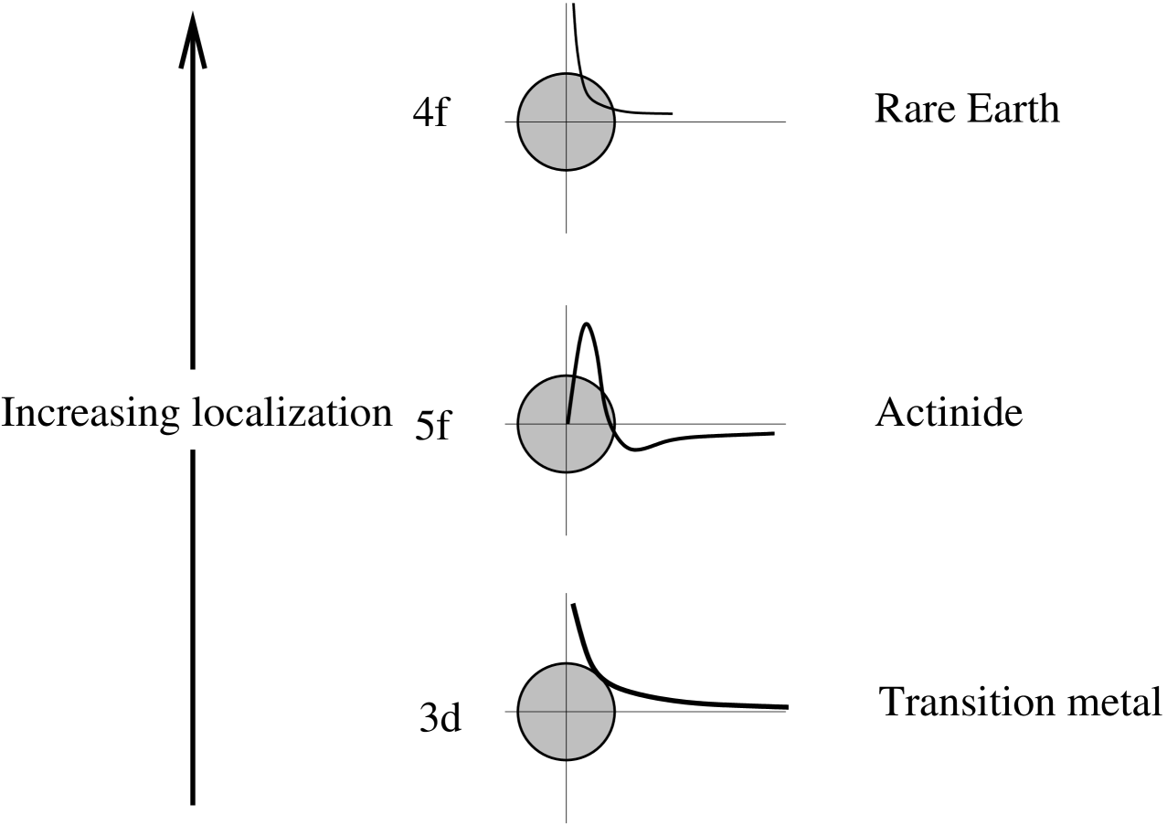
Figure 1: Depicting localized $4f$, $5f$ and $3d$ atomic wavefunctions.

Localized moments are the origin of magnetism in insulators, and in metals their interaction with the mobile charge carriers profoundly changes the nature of the metallic state via a mechanism known as the “Kondo effect”.

In the past decade, the physics of local moment formation has also reappeared in connection with quantum dots, where it gives rise to the Coulomb blockade phenomenon and the non-equilibrium Kondo effect.

1.2 Anderson’s Model of Local Moment Formation

Though the concept of localized moments was employed in the earliest applications of quantum theory to condensed matter, a theoretical understanding of the mechanism of moment formation did not develop until the early sixties, when experimentalists began to systematically study impurities in metals.

In the early 1960s, Clogston, Mathias and collaboratorsearlymagrefs showed that when small concentrations $n_{i}$ of magnetic ions, such as iron are added to a metallic host, they develop a Curie component to the magnetic susceptibilty

$$\chi=n_{i}{M^{2}\over 3T}\qquad\qquad M^{2}=g_{J}^{2}\mu_{B}^{2}J(J+1),$$ (1)

indicating the formation of a local moment. However, the local moment does not always develop, depending on the metallic host in which the magnetic ion was embedded. For example, iron dissolved at $1\%$ concentration in pure $Nb$ does not develop a local moment, but in the alloy $Nb_{1-x}Mo_{x}$ a local moment develops for $x>0.4$, rising to $2.2\mu_{B}$ above $x=0.9$. What is the underlying physics behind this phenomenon?

Andersonanda was the first to identify interactions between localized electrons as the driving force for local moment formation. Earlier work by FriedelFriedel and Blandinblandin had already identified part of the essential physics of local moments with the development of resonant bound-states. Anderson now included interactions to this picture. Much of the basic physics can be understood by considering an isolated atom with a localized $S=1/2$ atomic state which we shall refer to as a localized “d-state”. In isolation, the atomic bound state is stable and can be modeled in terms of a single level of energy $E_{d}$ and a Coulomb interaction

$$U=\frac{1}{2}\int d^{3}xd^{3}x^{\prime}V(\vec{x}-\vec{x}^{\prime})|\psi(\vec{x})|^{2}|\psi(\vec{x}^{\prime})|^{2},$$ (2)

where $V(\vec{x}-\vec{x}^{\prime})={e^{2}}/{4\pi\epsilon_{0}|\vec{x}-\vec{x^{\prime}}|}$ is the Coulomb potential.

The Anderson model for a localized impurity atom is given by

$$H=H_{c}+H_{mix}+\overbrace{H_{d}+H_{U}}^{H_{atomic}}$$ (3)

where $H_{d}=E_{d}\sum_{\sigma}\hat{n}_{d\sigma}$ describes an isolated atomic d-state of energy $E_{d}$ and occupancy $n_{d\sigma}$ in the “up” and “down” state. $H_{U}=U\hat{n}_{d\uparrow}\hat{n}_{d\downarrow}$ is the inter-atomic interaction between the up and down d-electrons. The term

$$H_{c}=\sum_{\vec{k}\sigma}\epsilon_{\vec{k}}c{{}^{{\dagger}}}_{\vec{k}\sigma}c_{\vec{k}\sigma}$$

describes the dispersion of electrons in the conduction sea which surrounds the ion, where $c{{}^{{\dagger}}}_{\vec{k}\sigma}$ creates an electron of momentum $\vec{k}$, spin $\sigma$ and energy $\epsilon_{\vec{k}}$. When the ion is embedded within a metal, the energy of the d-state is degenerate with band-electron states, and the term

$$H_{mix}=\sum_{j\sigma}\bigl{[}V_{\vec{k}}c{{}^{{\dagger}}}_{k\sigma}d_{\sigma}+{\rm H.c.}\bigr{]}$$

describes the hybridization that then takes place with the conduction electron sea, where $d{{}^{{\dagger}}}_{\sigma}$ describes the creation of a d-electron. The matrix element of the ionic potential between a plane wave conduction state and the d-orbital is

$$V_{\vec{k}}=\langle\vec{k}\sigma|\hat{V}|d^{1}\sigma^{\prime}\rangle=\int d^{3}re^{-i\vec{k}\cdot\vec{r}}V_{ion}(r)\psi(\vec{r})\delta_{\sigma\sigma^{\prime}}.$$ (4)

where $\psi(\vec{r})$ is the wavefunction of the localized orbital and $V_{ion}(r)$ is the ionic potential.This matrix element will have the same symmetry as the localized orbital- a matter of some importance for real d-states, or f-states . However, for the discussion that follows, the detailed $\vec{k}$ dependence of this object can essentially be ignored .

Let us first focus on the atomic part of H,

$$H_{atomic}=H_{d}+H_{U}=E_{d}\sum_{\sigma}\hat{n}_{d\sigma}+Un_{d\uparrow}n_{d\downarrow}.$$

The four states of this ion are

$$\begin{array}[]{rl}|d^{2}\rangle&E(d^{2})=2E_{d}+U\cr|d^{0}\rangle&E(d^{0})=0\cr|d^{1}\uparrow\rangle\quad|d^{1}\downarrow\rangle&E(d^{1})=E_{d}.\end{array}$$ (9)

To obtain a magnetic doublet as the ground-state, the excitation energies out of the doublet state must be greater than zero, i.e

$$E(d^{2})-E(d^{1})=E_{d}+U>0 \Rightarrow E_{d}+U/2>-U/2$$ (10)

$$E(d^{0})-E(d^{1})=-E_{d}>0 \Rightarrow U/2>E_{d}+U/2$$ (11)

so that for

$$U/2>|E_{d}+U/2|,$$

the isolated ion has a doubly degenerate magnetic ground-state, as illustrated in 2. We see that provided the Coulomb interaction $U$ is large enough compared with the level spacing, the ground-state of the ion becomes magnetic. The d-excitation spectrum of the ion will involve two sharp levels, one at energy $E_{d}$, the other at energy $E_{d}+U$.

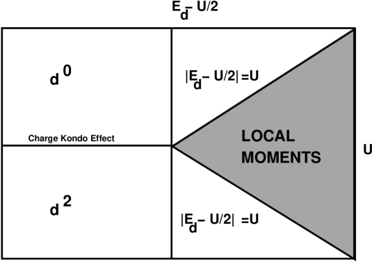
Figure 2: Phase diagram for Anderson Impurity Model in the Atomic Limit.

Suppose this ion is embedded in a metal: the free electron continuum is then pulled downwards by the work function of the metal so that now the d-level energy is degenerate with conduction electron energy levels. In this situation we expect the d-level to hybridize with the conduction electron states, broadening the sharp d-level into a resonance with a width $\Delta=\Delta(E_{d})$, where $\Delta(\epsilon)$ is given by Fermi’s Golden Rule.

$$\Delta(\epsilon)=\pi\sum_{\vec{k}}|V(\vec{k})|^{2}\delta(\epsilon_{\vec{k}}-\epsilon)=\pi\overline{N(\epsilon)V^{2}(\epsilon)}$$ (12)

where $N(\epsilon)=\sum_{\vec{k}}\delta(\epsilon_{\vec{k}}-\epsilon)$ is the electron density of states (per spin). In the discussion that follows, let us assume that over the energy width of the resonance, $V(\epsilon)$ and $N(\epsilon)\sim N(0)$ are essentially constant.

When this hybridization is small compared with $U$, we expect the ground-states of the ion to be essentially that of the atomic limit. For weak interaction strength $U$ the hybridization with the conduction sea will produce a single d-resonance of width $\Delta$ centered around $E_{d}$. In Anderson’s model for moment formation, when $U>U_{c}\sim\pi\Delta$ the single resonance splits into two, so that for large $U\gg U_{c}$, there are two d-resonances centered around $E_{d}$ and $E_{d}+U$, as shown in Fig. 3.

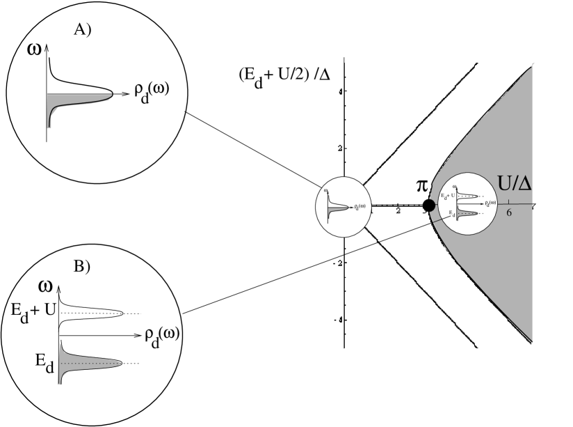
Figure 3: Illustrating how the d-electron resonance splits to form a local moment. A) $U<\pi\Delta$, single half-filled resonance. B) $U>\pi\Delta$, up and down components of the resonance are split by an energy $U$.

To illustrate the calculations that lead to this conclusion, let us use a Feynman diagram approach. We shall treat $H_{I}=H_{mix}+H_{U}$ as a perturbation to the non-interacting part of the Hamiltonian to be $H=H_{b}+H_{d}$. The Green’s functions of the bare d-electron and conduction electron are then denoted by

$$G^{0}(k,i\omega_{n})=[i\omega_{n}-\epsilon_{k}]^{-1}$$ (13)

(14)

$$G^{0}_{d}=[(i\omega_{n})-E_{d}]^{-1}$$

whilst the Feynman diagrams for the hybridization and the interaction terms are then

$$V^{*}(k)$$ (15)

(16)

$$V(k)$$ (17)

(18)

$$-U$$ (19)

Quite generally, the propagator for the d-electrons can be written

$$G_{d\sigma}(\omega)=[\omega-E_{d}-\Sigma_{d\sigma}(\omega)]^{-1}$$ (20)

where $\Sigma_{d\sigma}(\omega)$ is the the self-energy of the d-electron with spin $\sigma$. We delineate between “up” and “down”, anticipating Anderson’s broken symmetry description of a local moment as a resonance immersed in a self-consistently determined Weiss field. The density of states associated with the d-resonance is determined by the imaginary part of the d-Green function:

$$\rho_{d\sigma}(\omega)=\frac{1}{\pi}\hbox{Im}G_{d\sigma}(\omega-i\delta).$$ (21)

The Anderson model for local moment formation is equivalent to the Hartree approximation to the d-electron self-energy, denoted by

$$\qquad\quad\Sigma_{d\sigma}(\omega)\qquad=\ \ \qquad\Sigma_{1}(\omega)+\quad\qquad Un_{d-\sigma}$$

The first term in this expression derives from the hybridization of the d-electrons with the conduction sea. Notice that the d-state fluctuates into all k-states of the conduction sea, so that there is a sum over $k$ inside $\Sigma_{1}(\omega)$. The second term is the Hartree approximation to the interaction self energy. We can identify the fermion loop here as the occupancy of the $-\sigma$ d-state, so that

$$G_{d\sigma}(\omega)=[\omega-(E_{d}+Un_{d-\sigma})-\Sigma_{1}(\omega)]^{-1}$$ (22)

so the Hartree approximation is equivalent to replacing $E_{d}\rightarrow E_{d\sigma}=E_{d}+Un_{d,-\sigma}$. The hybridization part of the self energy is

$$\Sigma_{1}(\omega+i\delta)=\sum_{\vec{k}}\frac{|V(\vec{k})|^{2}}{\omega-\epsilon_{\vec{k}}-i\delta}$$

Notice that since $1/(x\mp i\delta)=P(1/x)\pm i\pi\delta(x)$, it follows that $Im\Sigma_{d}(\omega\pm i\delta)=\mp\Delta(\omega)$, so the imaginary part of this quantity has a discontinuity along the real axis equal to the hybridization width. Using (12), you can verify that we can now rewrite this as

$$\Sigma_{1}(\omega+i\delta) = \int\frac{d\epsilon}{\pi}{{\pi\sum_{\vec{k}}|V(\vec{k})|^{2}\delta(\epsilon_{\vec{k}}-\epsilon)}\over{\omega-\epsilon-i\delta}}$$ (23)

$$= \int\frac{d\epsilon}{\pi}{\Delta(\epsilon)\over{\omega-\epsilon}-i\delta}$$ (24)

Typically $\Delta(\epsilon)$ will only vary substantially on energies of order the bandwidth, so that over the width of the resonance we can replace $\Delta(\epsilon)\rightarrow\Delta$. Moreover, for a broad band of width $D$, the real part of $\Sigma(\omega)\sim\frac{1}{\pi}\Delta(0)\ln[(\omega-D)/(\omega+D)]$ is of order $\omega/D$ and can be ignored, or absorbed into into a small renormalization of $E_{d}$. This allows us to make the replacement

$$\Sigma_{1}(\omega\pm i\delta)=\mp i\Delta{\rm sgn\delta}$$

so that

$$G_{d\sigma}(\omega-i\delta)={1\over(\omega-E_{d\sigma}-i\Delta)}.$$ (25)

The density of states described by the Green-function is a Lorentzian centered around energy $E_{d\sigma}$:

$$\rho_{d\sigma}(\omega)=\frac{1}{\pi}ImG_{d\sigma}(\omega-i\delta)=\frac{\Delta}{(\omega-E_{d\sigma})^{2}+\Delta^{2}},$$

moreover, the occupancy of the d-state is given by the d-occupation at zero temperature is

$$\begin{array}[]{rcl}n_{d\sigma}&=&\int_{-\infty}^{0}d{\omega}\rho_{d\sigma}(\omega)\cr&=&\frac{1}{\pi}\cot^{-1}\left(\frac{E_{d}+Un_{d-\sigma}}{\Delta}\right)\end{array}$$ (26)

This equation defines Anderson’s mean-field theory. It is convenient to introduce an occupancy $n_{d}=\sum_{\sigma}n_{d\sigma}$ and magnetization $M=n_{d\uparrow}-n_{d\downarrow}$, so that $n_{d\sigma}=\frac{1}{2}(n_{d}+\sigma M)$ ($\sigma=\pm 1$). The mean-field equation for the occupancy and magnetization are then

$$n_{d} = \frac{1}{\pi}\sum_{\sigma=\pm 1}\cot^{-1}\left(\frac{E_{d}+U/2(n_{d}-\sigma M)}{\Delta}\right)$$ (27)

$$M = \frac{1}{\pi}\sum_{\sigma=\pm 1}\sigma\cot^{-1}\left(\frac{E_{d}+U/2(n_{d}-\sigma M)}{\Delta}\right)$$ (28)

To find the critical size of the interaction strength where a local moment develops, set $M\rightarrow 0^{+}$ (replacing the second equation by its derivative w.r.t. $M$), which gives

$$n_{d} = \frac{2}{\pi}\cot^{-1}\left(\frac{E_{d}+U_{c}n_{d}/2}{\Delta}\right)$$ (29)

$$1 = \frac{U_{c}}{\pi\Delta}\frac{1}{1+\left(\frac{E_{d}+Un_{d}/2}{\Delta}\right)^{2}}$$ (30)

which can be written parametrically as

$$E_{d}+\frac{U_{c}}{2} = \Delta\left(c+\frac{\pi}{2}(1-n_{d})(1+c^{2})\right)$$ (31)

$$U_{c} = \pi\Delta(1+c^{2})$$ (32)

where $c\equiv\cot\left(\frac{\pi n_{d}}{2}\right).$ The critical curve described by these equations is shown in Fig. 3.

From the mean-field equations, it is easily seen that for $n_{d}=1$, when the d-levels are half filled, the critical value $U_{c}=\pi\Delta$. This enables us to qualitatively understand the experimentally observed formation of local moments. When dilute magnetic ions are dissolved into a metallic host, the formation of a local moment is dependent on whether the ratio $U/\pi\Delta$ is larger than, or smaller than zero. When iron is dissolved in pure niobium, the failure of the moment to form reflects the higher density of states and larger value of $\Delta$ in this alloy. When iron is dissolved in molybdenum, the lower density of states causes $U>U_{c}$, and local moments form. earlymagrefs

1.2.1 The Coulomb Blockade

A modern context for the physics of local moments is found within quantum dots. A quantum dot is a tiny electron pool in a doped semi-conductor, small enough so that the electron states inside the dot are quantized, loosely resembling the electronic states of an atom. Unlike a conventional atom, the separation of the electronic states is of the order of milli-electron volts, rather than volts. The overall position of the quantum dot energy levels can be changed by applying a gate voltage to the dot. It is then possible to pass a small current through the dot by placing it between two leads. The differential conductance $G=dI/dV$ is directly proportional to the density of states $\rho(\omega)$ inside the dot $G\propto\rho(0)$. Experimentally, when G is measured as a function of gate voltage $V_{g}$, the differential conductance is observed to develop a periodic structure, with a period of a few milli-electron volts. qdots

This phenomenon is known as the “Coulomb blockade” and it results from precisely the same physics that is responsible for moment formation. A simple model for a quantum dot considers it as a sequence of single particle levels at energies $\epsilon_{\lambda}$, interacting via a single Coulomb potential $U$, according to the model

$$H_{dot}=\sum_{\lambda}(\epsilon_{\lambda}-eV_{g})n_{\lambda\sigma}+\frac{U}{2}N(N-1)$$ (33)

where $n_{\lambda\sigma}$ is the occupancy of the spin $\sigma$ state of the $\lambda$ level, $N=\sum_{\lambda\sigma}n_{\lambda\sigma}$ is the total number of electrons in the dot and $V_{g}$ the gate voltage. This is a simple generalization of the single atom part of the Anderson model. Notice that the capacitance of the dot is $C=e^{2}/U$.

Provided that $U$ is far greater than the energy separation of the individual levels, $U>>\epsilon_{\lambda}-\epsilon_{\lambda^{\prime}}$, the energy difference between the $n$ electron and $n+1$ electron state of the dot is given by $E(n+1)-E(n)=nU-eV_{g}$. As the gate voltage is raised, the quantum dot fills each level sequentially, as illustrated in Fig. 4, and when $eV_{g}=U$, the n-th level becomes degenerate with the Fermi energy of each lead. At this point, electrons can pass coherently through the resonance giving rise to a sharp peak in the conductance. At maximum conductance, the transmission and reflection of electrons is unitary, and the conductance of the quantum dot will reach a substantial fraction of the quantum of conductance, $e^{2}/h$ per spin. A simple calculation of the zero-temperature conductance through a single non-interacting resonance coupled symmetrically to two leads gives

$$G(eV_{g})=\frac{2e^{2}}{h}\frac{\Delta^{2}}{(E_{\lambda}-eV_{g})^{2}+\Delta^{2}}$$ (34)

where the factor of two derives from two spin channels. At finite temperatures, the resonance becomes broadened by thermal excitation effects, giving

$$G(eV_{g},T)=\frac{2e^{2}}{h}\int d\epsilon\left(-\frac{df(\epsilon-eV_{g})}{d\epsilon}\right)\frac{\Delta^{2}}{(E_{\lambda}-\epsilon)^{2}+\Delta^{2}}$$

where $f(\epsilon)=1/(e^{\beta\epsilon}+1)$ is the Fermi function. When interactions are included, we must sum over the n-levels, giving (See Fig. 4. )

$$G(eV_{g},T)=\frac{2e^{2}}{h}\int d\epsilon\left(-\frac{df(\epsilon-eV_{g})}{d\epsilon}\right)\frac{\Delta^{2}}{(nU-\epsilon)^{2}+\Delta^{2}}$$

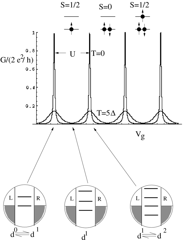
Figure 4: Variation of zero bias conductance $G=dI/dV$ with gate voltage in a quantum dot. Coulomb interactions mean that for each additional electron in the dot, the energy to add one electron increases by $U$. When the charge on the dot is integral, the Coulomb interaction blocks the addition of electrons and the conductance is suppressed. When the energy to add an electron is degenerate with the Fermi energy of the leads, unitary transmission occurs, and for symmetric leads, $G=2e^{2}/h$.

The effect of field on these results is interesting. When the number of electrons in the dot is even, the quantum dot is in a singlet state. When the number of electrons is odd, the quantum dot forms a local moment. In a magnetic field, the energy of the odd-electron dot is reduced, whereas the energy of the even spin dot is unchanged, with the result that at low temperatures

$$E(2n+1)-E(2n) = 2nU-\mu_{B}B$$ (35)

$$E(2n+2)-E(2n+1) = (2n+1)U+\mu_{B}B$$ (36)

so that the voltages of the odd and even numbered peaks in the conductance develop an alternating field dependence.

It is remarkable that the physics of moment formation and the “Coulomb blockade” operate in both artificial mesoscopic devices and naturally occurring magnetic ions.

1.3 Exercises

1. By expanding a plane wave state in terms of spherical harmonics:

   $$\langle\vec{r}|\vec{k}\rangle=e^{i\vec{k}\cdot\vec{r}}=4\pi\sum_{l,m}i^{l}j_{l}(kr)Y^{*}_{lm}(\hat{k})Y_{lm}(\hat{r})$$

   show that the overlap between a state $|\psi\rangle$ with wavefunction $\langle\vec{x}|\psi\rangle=R(r)Y_{lm}(\hat{r})$ with a plane wave is given by $V(\vec{k})=\langle\vec{k}|V|\psi\rangle=V(k)Y_{lm}(\hat{k})$ where

   $$V(k)=4\pi i^{-l}\int drr^{2}V(r)R(r)j_{l}(kr)$$ (37)

2. • Show that $\delta=\cot^{-1}\left(\frac{E_{d}}{\Delta}\right)$ is the scattering phase shift for scattering off a resonant level at position $E_{d}$.

   • Show that the energy of states in the continuum is shifted by an amount $-\Delta\epsilon\delta(\epsilon)/\pi$, where $\Delta\epsilon$ is the separation of states in the continuum.

   • Show that the increase in density of states is given by $\partial\delta/\partial E=\rho_{d}(E)$. (See chapter 3.)

3. Derive the formula (34) for the conductance of a single isolated resonance.

2 The Kondo Effect

Although Anderson’s mean-field theory provided a mechanism for moment formation, it raised many new questions. One of its inadequacies is that of the magnetic moment is regarded as a broken symmetry order parameter. Broken symmetry is possible when the object that breaks the symmmetry involves a macroscopic number of degrees of freedom, but here, we are dealing with a single spin. There will always be a certain quantum mechanical amplitude for the spin to flip between an up and down configuration. This tunneling rate $\tau^{-1}$ defines a temperature scale

$$k_{B}T_{K}=\frac{{\mathchar 22\relax\mkern-9.0muh}}{\tau}$$

called the Kondo temperature, which sets the dividing line between local moment behavior, where the spin is free, and the low temperature limit, where the spin becomes highly correlated with the surrounding electrons. Experimentally, this temperature marks the low temperature limit of a Curie susceptibility. The physics by which the local moment disappears or “quenches” at low temperatures is closely analagous to the physics of quark confinement and it is named the “Kondo effect” after the Japanese physicist Jun Kondo. kondo

The Kondo effect has a wide range of manifestations in condensed matter physics: not only does it govern the quenching of magnetic moments inside a metal, but it also is responsible for the formation of heavy fermion metals, where the local moments transform into composite quasiparticles with masses sometimes in excess of a thousand bare electron masses.stewart Recently, the Kondo effect has also been observed to take place in quantum dots that carry a local moment. (Typically quantum dots with an odd number of electrons). qdots

In this section we will first derive the Kondo model from the Anderson model, and then discuss the properties of this model in the language of the renormalization group .

2.1 Adiabaticity

Let us discuss some of the properties of the Anderson model at low temperatures using the idea of adiabaticity. We suppose that the interaction between electrons in the Anderson model is increased continuously to values $U>>\Delta$, whilst maintaining the occupancy of the d-state equal to unity $n_{d}=1$. The requirement that $n_{d}=1$ ensures that the d-electron density of states is particle-hole symmetric, which implies that $E_{d}=0$ and $\Sigma^{\prime}(0)=0$.

When $U>>\Delta$, we expect that the d-electron spectral function $\rho_{d}=\frac{1}{\pi}\hbox{Im}G_{d}(\omega-i\delta)$ will contain two peaks at $\omega=\pm U/2$. Since the total spectral weight integrates to unity, $\int d\omega\rho(\omega)=1$, we expect that the weight under each of these peaks is approximately $1/2$. Remarkably, as we shall now see, the spectral function at $\omega=0$ is unchanged by the process of increasing the interaction strength and remains equal to its non-interacting value

$$\rho_{d}(\omega=0)=\frac{1}{\Delta}$$

This means that the d-spectral function must contain a narrow peak, of vanishingly small spectral weight $Z<<1$, height $\frac{1}{\Delta}$ and hence width $\Delta^{*}=Z\Delta<<\Delta$. This peak in the d-spectral function is associated with the Kondo effect, and is known as the Abrikosov-Suhl, or the “Kondo” resonance.

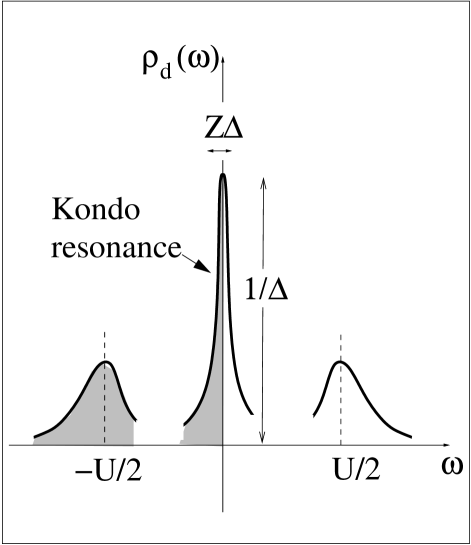
Figure 5: “Kondo resonance” in the d-spectral function. At large $U$ for the particle hole-symmetric case where $n_{d}=1$, the d-spectral function contains two peaks about $\omega\sim\pm U/2$, both of weight approximately $1/2$. However, since the spectral function is constrained by the requirement that $\rho_{d}(\omega=0)=\frac{1}{\Delta}$, the spectral function must preserve a narrow peak of fixed height, but vanishingly small weight $Z<<1$.

Let us see how this comes about as a consequence of adiabaticity. For a single magnetic ion, we expect that the interactions between electrons can be increased continuously, without any risk of instabilities, so that the excitations of the strongly interacting case remain in one-to-one correspondence with the excitations of the non-interacting case $U=0$, forming a “local Fermi liquid”.

In this local Fermi liquid, one can divide the d-electron self-energy into two components- the first derived from hybridization, the second derived from interactions:

$$\Sigma(\omega-i\delta) = i\Delta+\Sigma_{I}(\omega-i\delta)$$ (38)

$$\Sigma_{I}(\omega-i\delta) = (1-Z^{-1})\omega+iA\omega^{2}.$$ (39)

The “wavefunction” renormalization $Z$ is less than unity. The quadratic energy dependence of $\Sigma_{I}(\omega)\sim\omega^{2}$ follows from the quadratic energy dependence of the phase space for producing particle-hole pairs. Using this result, the form of the d-electron propagator for $n_{d}$ at low energies is

$$G_{d}(\omega-i\delta) = \frac{1}{\omega-i\Delta-\Sigma_{I}(\omega)}$$ (40)

$$= \frac{Z}{\omega-iZ\Delta-iO(\omega^{2}).}$$ (41)

This corresponds to a renormalized resonance of reduced weight $Z<1$, renormalized width $Z\Delta$. One of the remarkable results of this line of reasoning, is the discovery that d-spectral weight

$$\rho_{d}(\omega\sim 0)=\frac{1}{\pi}{\rm Im}G_{d}(\omega-i\delta)|_{\omega=0}=\frac{1}{\Delta}$$

is independent of the strength of $U$. This result, first discovered by Langrethlangreth guarantees a peak in the d-spectral function at low energies, no matter how large $U$ becomes. Since we also expect a peak in the d-spectral function around $\omega\sim\pm U/2$, this line of reasoning suggests that the structure of the d-spectral function at large $U$, contains three peaks.

2.2 Schrieffer-Wolff transformation

If a local moment forms within an atom, the object left behind is a pure quantum top- a quantum mechanical object with purely spin degrees of freedom.

These spin degrees of freedom do interact with the surrounding conduction sea. In particular virtual charge fluctuations, in which an electron briefly migrates off, or onto the ion lead to spin-exchange between the local moment and the conduction sea. This induces an antiferromagnetic interaction between the local moment and the conduction electrons. To see this consider the two possible spin exchange processes

$$e_{\uparrow}+d^{1}_{{\downarrow}} \leftrightarrow d^{2}\leftrightarrow e_{\downarrow}+d^{1}_{{\uparrow}}\qquad\Delta E_{I}\sim U+E_{d}$$ (42)

$$e_{\uparrow}+d^{1}_{{\downarrow}} \leftrightarrow e_{{\uparrow}}+e_{\downarrow}\leftrightarrow e_{\downarrow}+d^{1}_{{\uparrow}}\qquad\Delta E_{II}\sim-E_{d}$$ (43)

The first process passes via a doubly occupied singlet d-state, so it can only take place if the incoming conduction electron and d-electron are in a mutual $S=0$ state. In the second process, in order that the conduction electron can hybridize with the d-state, it has to arrive and depart in a state with precisely the same d- orbital symmetry. This means that the intermediate state formed in the second process must be spatially symmetric, and must therefore be a spin-antisymmetric singlet $S=0$ state. From these arguments, we see that spin exchange only takes place in the singlet channel, lowering the energy of the singlet configurations by an amount of order

$$J \sim V^{2}\left[\frac{1}{\Delta E_{1}}+\frac{1}{\Delta E_{2}}\right]$$ (44)

$$= \left[\frac{1}{-E_{d}}+\frac{1}{E_{d}+U}\right]$$ (45)

where $V$ is the size of the hybridization matrix element near the Fermi surface. If we introduce the electron spin density operator $\vec{S}(0)=\frac{1}{N}\sum_{k,k^{\prime}}c{{}^{{\dagger}}}_{k\alpha}\vec{\sigma}_{\alpha\beta}c_{k^{\prime}\beta}$, where $N$ is the number of sites in the lattice, then we expect that the effective interaction induced by the virtual charge fluctuations will have the form

$$H_{eff}=J\vec{S}(0)\cdot\vec{S}_{d}$$

where $\vec{S}_{d}$ is the spin of the localized moment. Notice that the sign of $J$ is antiferromagnetic. This kind of heuristic argument was ventured in Anderson’s paper on local moment formation in 1961. The antiferromagnetic sign in this interaction was quite unexpected, for it had been tacitly assumed by the community that exchange forces would induce a ferromagnetic interaction between the conduction sea and local moments. This seemingly innocuous sign difference has deep consequences for the physics of local moments at low temperatures, as we shall see in the next section.

Let us now carry out the transformation a little more carefully, using the method of canonical transformations introduced by Schrieffer and Wolffswolf ; coqblin . The Schrieffer-Wolff transformation is very close to the idea of the renormalization group and will help set up our renormalization group discussion. When a local moment forms, the hybridization with the conduction sea induces virtual charge fluctuations. It is therefore useful to consider dividing the Hamiltonian into two terms

$$H=H_{1}+\lambda{\mathcal{V}}$$

where $\lambda$ is an expansion parameter. Here,

$$H_{1}=H_{band}+H_{atomic}=\left[{\hbox{${{{\displaystyle\raisebox{4.0pt}{$H_{L}$}\above 1.0pt\displaystyle\raisebox{-4.0pt}{$\ \ 0\ \ \ $}}}}$}\left|{\bf{{\displaystyle\raisebox{0.0pt}{$\ 0$}\above 1.0pt\displaystyle\raisebox{0.0pt}{$H_{H}$}}}}\right.}\right]$$

is diagonal in the low energy $d^{1}$ ($H_{L}$) and the high energy $d^{2}$ or $d^{0}$ ($H_{H}$) subspaces, whereas the hybridization term

$$\mathcal{V}=H_{mix}=\sum_{j\sigma}\bigl{[}V_{\vec{k}}c{{}^{{\dagger}}}_{k\sigma}d_{\sigma}+{\rm H.c.}\bigr{]}=\left[{\hbox{${{{\displaystyle\raisebox{4.0pt}{$\ \ 0\ $}\above 1.0pt\displaystyle\raisebox{-4.0pt}{$V$}}}}$}\left|{\bf{{\displaystyle\raisebox{0.0pt}{$V{{}^{{\dagger}}}$}\above 1.0pt\displaystyle\raisebox{0.0pt}{$0$}}}}\right.}\right]$$

provides the off-diagonal matrix elements between these two subspaces. The idea of the Schrieffer Wolff transformation is to carry out a canonical transformation that returns the Hamiltonian to block-diagonal form, as follows:

$$U\left[{\hbox{${{{\displaystyle\raisebox{4.0pt}{$H_{L}$}\above 1.0pt\displaystyle\raisebox{-4.0pt}{$\lambda V$}}}}$}\left|{\bf{{\displaystyle\raisebox{0.0pt}{$\lambda V{{}^{{\dagger}}}$}\above 1.0pt\displaystyle\raisebox{0.0pt}{$H_{H}$}}}}\right.}\right]U{{}^{{\dagger}}}=\left[{\hbox{${{{\displaystyle\raisebox{4.0pt}{$H^{*}$}\above 1.0pt\displaystyle\raisebox{-4.0pt}{$0$}}}}$}\left|{\bf{{\displaystyle\raisebox{0.0pt}{$0\phantom{{{}^{{\dagger}}}}$}\above 1.0pt\displaystyle\raisebox{0.0pt}{$H^{\prime}$}}}}\right.}\right].$$ (46)

This is a “renormalized” Hamiltonian, and the block-diagonal part of this matrix $H^{*}=P_{L}H^{\prime}P_{L}$ in the low energy subspace provides an effective Hamiltonian for the low energy physics and low temperature thermodynamics. If we set $U=e^{S}$, where $S=-S{{}^{{\dagger}}}$ is anti-hermitian and expand S in a power series

$$S=\lambda S_{1}+\lambda^{2}S_{2}+\dots,$$

then expanding (46) using the identity $e^{A}Be^{-A}=B+[A,B]+\frac{1}{2!}[A,[A,B]]\dots$

$$e^{S}(H_{1}+\lambda{\mathcal{V}})e^{-S}=H_{1}+\lambda\left(\mathcal{V}+[S_{1},H_{1}]\right)+\lambda^{2}\left(\frac{1}{2}[S_{1},[S_{1},H]]+[S_{1},\mathcal{V}]+[S_{2},H_{1}]\right)+\dots$$

so that to leading order

$$[S_{1},H_{1}]=-\mathcal{V},$$ (47)

and to second order

$$e^{S}(H_{1}+\lambda{\mathcal{V}})e^{-S}=H_{1}+\lambda^{2}\left(\frac{1}{2}[S_{1},\mathcal{V}]+[S_{2},H_{1}]\right)+\dots.$$

Since $[S_{1},\mathcal{V}]$ is block-diagonal, we can satisfy (46 ) to second order by requiring $S_{2}=0$, so that to this order, the renormalized Hamiltonian has the form (setting $\lambda=1$)

$$H^{*}=H_{L}+H_{int}$$

where

$$H_{int}=\frac{1}{2}P_{L}[S_{1},\mathcal{V}]P_{L}+\dots$$

is an interaction term induced by virtual fluctuations into the high-energy manifold. Writing

$$S=\left[{\hbox{${{{\displaystyle\raisebox{4.0pt}{$0$}\above 1.0pt\displaystyle\raisebox{-4.0pt}{$s$}}}}$}\left|{\bf{{\displaystyle\raisebox{0.0pt}{$-s{{}^{{\dagger}}}$}\above 1.0pt\displaystyle\raisebox{0.0pt}{$0$}}}}\right.}\right]$$

and substituting into (47), we obtain $V=-sH_{L}+H_{H}s$. Now since $(H_{L})_{{ab}}=E^{{L}}_{a}\delta_{ab}$ and $(H_{H})_{{ab}}=E^{{H}}_{a}\delta_{ab}$ are diagonal, it follows that

$$s_{ab}=\frac{V_{ab}}{E_{a}^{H}-E_{b}^{L}},\qquad-s{{}^{{\dagger}}}_{ab}=\frac{V{{}^{{\dagger}}}_{ab}}{E_{a}^{L}-E_{b}^{H}},\qquad.$$ (48)

From (48), we obtain

$$(H_{int})_{ab}=-\frac{1}{2}(V{{}^{{\dagger}}}s+s{{}^{{\dagger}}}V)_{ab}=\frac{1}{2}\sum_{\lambda\in|H\rangle}\left[\frac{V{{}^{{\dagger}}}_{a\lambda}V_{\lambda b}}{E_{a}^{L}-E_{\lambda}^{H}}+\frac{V{{}^{{\dagger}}}_{a\lambda}V_{\lambda b}}{E_{b}^{L}-E_{\lambda}^{H}}\right]$$

Some important points about this result

• We recognize this result as a simple generalization of second-order perturbation theory which encompasses off-diagonal matrix elements.

• $H_{int}$ can also be written

  $$H_{int}=\frac{1}{2}[T(E_{a})+T(E_{b})]$$

  where $T$ is given by

  $$\hat{T}(E) = P_{L}{\mathcal{V}}\frac{P_{H}}{E-H_{1}}{\mathcal{V}}P_{L}$$ (49)

  $$T_{ab}(E) = \sum_{\lambda\in|H\rangle}\left[\frac{V{{}^{{\dagger}}}_{a\lambda}V_{\lambda b}}{E-E_{\lambda}^{H}}\right]$$ (50)

  is the leading order expression for the scattering T-matrix induced by scattering off $\mathcal{V}$. We can thus relate $H_{int}$ to a scattering amplitude, and schematically represent it by a Feynman diagram, illustrated in Fig. 6.

  

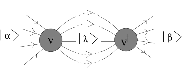
  Figure 6: T-matrix representation of interaction induced by integrating out high-energy degrees of freedom

• If the separation of the low and high energy subspaces is large, then the energy denominators in the above expression will not depend on the initial and final states $a$ and $b$, so that this expression can be simplified to the form

  $$H_{int}=-\sum_{\lambda\in|H\rangle}\frac{V{{}^{{\dagger}}}P_{\lambda}V}{\Delta E_{\lambda}}$$

  where $\Delta E_{\lambda}=E^{H}_{\lambda}-E^{L}$ is the excitation energy in the high energy subspace labeled by $\lambda$, and the projector $P_{\lambda}=\sum_{|a\rangle\in|\lambda\rangle}|a\rangle\langle a|$ .

If we apply this method to the Anderson model, we have two high-energy subspaces, with excitation energies $\Delta E(d^{1}\rightarrow d^{0})=-E_{d}$ and $\Delta E(d^{1}\rightarrow d^{2})=E_{d}+U$, so that the renormalized interaction is

$$H_{int}=-\sum_{k\sigma,k^{\prime}\sigma^{\prime}}V^{*}_{k^{\prime}}V_{k}\Biggl{[}\overbrace{\frac{(c{{}^{{\dagger}}}_{k\sigma}d_{\sigma})(d{{}^{{\dagger}}}_{\sigma^{\prime}}c_{k^{\prime}\sigma^{\prime}})}{E_{d}+U}}^{d^{1}+e^{-}\leftrightarrow d^{2}}+\overbrace{\frac{(d{{}^{{\dagger}}}_{\sigma^{\prime}}c_{k^{\prime}\sigma^{\prime}})(c{{}^{{\dagger}}}_{k\sigma}d_{\sigma})}{-E_{d}}}^{d^{1}\leftrightarrow d^{0}+e^{-}}\Biggr{]}$$

Using the identity $\delta_{ab}\delta_{cd}+\vec{\sigma}_{ab}\cdot\vec{\sigma}_{cd}=2\delta_{ad}\delta_{bc}$ we may cast the renormalized Hamiltonian in the form

$$H_{int} = \sum_{k\alpha,k^{\prime}\beta}J_{k,k^{\prime}}c{{}^{{\dagger}}}_{k\alpha}\vec{\sigma}c_{k^{\prime}\beta}\cdot\vec{S}_{d}+H^{\prime}$$ (51)

$$J_{k,k^{\prime}} = V^{*}_{k^{\prime}}V_{k}\Biggl{[}\overbrace{\frac{1}{E_{d}+U}}^{{d^{1}+e^{-}\leftrightarrow d^{2}}}+\overbrace{\frac{1}{-E_{d}}}^{d^{1}\leftrightarrow d^{0}+e^{-}}\Biggr{]}$$ (52)

where

$$\vec{S}_{d}\equiv d{{}^{{\dagger}}}_{\sigma}\left(\frac{\vec{\sigma}_{\alpha\beta}}{2}\right)d_{\beta},\qquad(n_{d}=1)$$ (53)

where we have replaced $n_{d}=1$ in the low energy subspace. Apart from a constant, the second term

$$H^{\prime}=-\frac{1}{2}\sum_{k,k^{\prime}\sigma}V^{*}_{k^{\prime}}V_{k}\left[\frac{1}{E_{d}+U}+\frac{1}{E_{d}}\right]c{{}^{{\dagger}}}_{k\sigma}c_{k^{\prime}\sigma}$$

is a residual potential scattering term off the local moment. This term vanishes for the particle-hole symmetric case $E_{d}=-(E_{d}+U)$ and will be dropped, since it does not involve the internal dynamics of the local moment. Summarizing, the effect of the high-frequency valence fluctuations is to induce an antiferromagnetic coupling between the local spin density of the conduction electrons and the local moment:

$$H=\sum_{k\sigma}\epsilon_{k}c{{}^{{\dagger}}}_{k\sigma}c_{k\sigma}+\sum_{k,k^{\prime}}J_{k,k^{\prime}}c{{}^{{\dagger}}}_{k\alpha}\vec{\sigma}c_{k^{\prime}\beta}\cdot\vec{S}_{d}$$ (54) This is the infamous “Kondo model”. For many purposes, the $k$ dependence of the coupling constant can be dropped. In this case, the Kondo interaction can be written $H_{int}=J\psi{{}^{{\dagger}}}(0)\vec{\sigma}\psi(0)\cdot\vec{S}_{d}$, where $\psi_{\alpha}(0)=\frac{1}{\sqrt{N}}\sum c_{k\alpha}$ is the electron operator at the origin and $\psi{{}^{{\dagger}}}(0)\vec{\sigma}\psi(0)$ is the spin density at the origin. In this simplified form, the Kondo model takes the deceptively simple form

$$H=\sum_{k\sigma}\epsilon_{k}c{{}^{{\dagger}}}_{k\sigma}c_{k\sigma}+\overbrace{J\psi{{}^{{\dagger}}}(0)\vec{\sigma}\psi(0)\cdot\vec{S}_{d}}^{{H_{int}}}.$$ (55)

In other words, there is a simple point-interaction between the spin density of the metal at the origin and the local moment. Notice how all reference to the fermionic character of the d-electrons has gone, and in their place, is a $S=1/2$ spin operator. The fermionic representation (53) of the spin operator proves to be very useful in the case where the Kondo effect takes place.

2.3 Renormalization concept

To make further progress, we need to make use of the concept of renormalization. In a general sense, physics occurs on several widely spaced energy scales in condensed matter systems. We would like to distill the essential effects of the high energy atomic physics at electron volt scales on the low energy physics at millivolt scales without getting caught up in the fine details. An essential tool for this task is the “renormalization group”. yuval ; poor ; wilson ; Noz

The concept of the renormalization group permits us to describe complex condensed matter systems using simple models that reproduce only the relevant low energy physics of the system. The idea here is that only certain gross features of the high energy physics are relevant to the low energy excitations. The continuous family of model Hamiltonians with the same low energy excitation spectrum constitute a “universality class” of models. (Fig. 7) Suppose we parameterize each model Hamiltonian $H(D)$ by its cutoff energy scale, $D$, the energy of the largest excitations. The scaling procedure, involves rescaling the cutoff $D\rightarrow D^{\prime}=D/b$ where $b>1$, integrating out the excitations $E\in[D^{\prime},D]$ to obtain an effective Hamiltonian $\tilde{H_{L}}$for the remaining low-energy degrees of freedom. The energy scales are then rescaled, to obtain a new $H(D^{\prime})=b\tilde{H_{L}}$ Generically, the Hamiltonian will have the block-diagonal form

$$H=\left[{\hbox{${{{\displaystyle\raisebox{4.0pt}{$H_{L}$}\above 1.0pt\displaystyle\raisebox{-4.0pt}{$V$}}}}$}\left|{\bf{{\displaystyle\raisebox{0.0pt}{$V{{}^{{\dagger}}}$}\above 1.0pt\displaystyle\raisebox{0.0pt}{$H_{H}$}}}}\right.}\right]$$ (56)

where $H_{L}$ and $H_{H}$ act on states in the low-energy and high-energy subspaces respectively, and $V$ and $V{{}^{{\dagger}}}$ provide the matrix elements between them. The high energy degrees of freedom may be “integrated out” by carrying out a canonical transformation and projecting out the low-energy component $\tilde{H}_{L}$

$$H(D)\rightarrow UH(D)U{{}^{{\dagger}}}=\left[{\hbox{${{{\displaystyle\raisebox{4.0pt}{$\tilde{H_{L}}$}\above 1.0pt\displaystyle\raisebox{-4.0pt}{$0$}}}}$}\left|{\bf{{\displaystyle\raisebox{0.0pt}{$0$}\above 1.0pt\displaystyle\raisebox{0.0pt}{$\tilde{H_{H}}$}}}}\right.}\right]$$ (57)

By rescaling

$$H(D^{\prime})=b\tilde{H_{L}}$$ (58)

one arrives at a new Hamiltonian describing the physics on the reduced scale. The transformation from $H(D)$ to $H(D^{\prime})$ is referred to as a “renormalization group” (RG) transformation. This term was coined long ago, even though the transformation does not form a real group, since there is no inverse transformation. Repeated application of the RG procedure

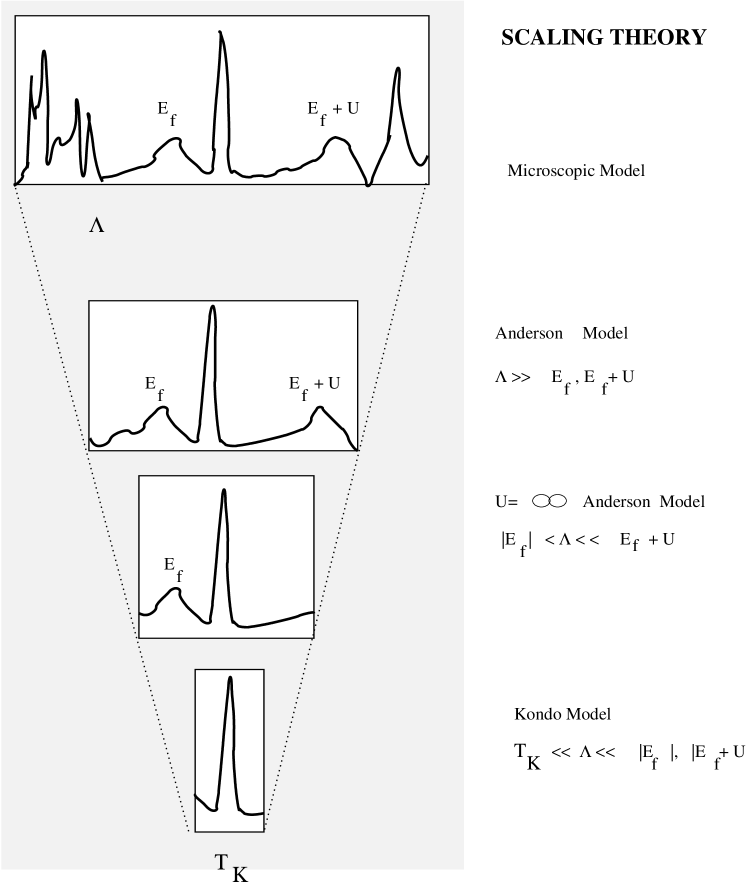
Figure 7: Scaling concept. Low energy model Hamiltonians are obtained from the detailed original model by integrating out the high energy degrees of freedom. At each stage, the physics described by the model spans a successively lower frequency window in the excitation spectrum.

leads to a family of Hamiltonians $H(D)$. By taking the limit $b\rightarrow 1$, these Hamiltonians evolve continuously with $D$. Typically, $H$ will contain a series of dimensionless coupling constants $\{g_{i}\}$ which denote the strength of various interaction terms in the Hamiltonian. The evolution of these coupling constants with cut-off is given by a scaling equation, so that for the simplest case

$$\frac{\partial g_{j}}{\partial\ln D}=\beta_{j}(\{g_{i}\})$$

A negative $\beta$ function denotes a “relevant” coupling constant which grows as the cut-off is reduced. A positive $\beta$ function denotes an “irrelevant” coupling constant which diminishes as the cut-off is reduced. There are two types of event that can occur in such a scaling procedure (Fig. 8):

• i) A crossover. When the cut-off energy scale $D$ becomes smaller than the characteristic energy scale of a particular class of high frequency excitations, then at lower energies, these excitations may only occur via a virtual process. To accommodate this change, the Hamiltonian changes its structure, acquiring additional terms that simulate the effect of the high frequency virtual fluctuations on the low energy physics. The passage from the Anderson to the Kondo model is an example of one such cross-over. In the renormalization group treatment of the Anderson model, when the band-width of the conduction electrons becomes smaller than the energy to produce a valence fluctuation, a cross-over takes place in which real charge fluctuations are eliminated, and the physics at all lower energy scales is described by the Kondo model.

• ii) Fixed Point. If the cut-off energy scale drops below the lowest energy scale in the problem, then there are no further changes to occur in the Hamiltonian, which will now remain invariant under the scaling procedure (so that the $\beta$ function of all remaining parameters in the Hamiltonian must vanish). This “Fixed Point Hamiltonian” describes the essence of the low energy physics.

2.4 “Poor Man” Scaling

We shall now apply the scaling concept to the Kondo model. This was originally carried out by Anderson and Yuval using a method formulated in the time, rather than energy domain. The method presented here follows Anderson’s “ Poor Man’s” scaling approach, in which the evolution of the coupling constant is followed as the band-width of the conduction sea is reduced. The Kondo model is written

$$H = \sum_{|\epsilon_{k}|<D}\epsilon_{k}c{{}^{{\dagger}}}_{k\sigma}c_{k\sigma}+H^{(I)}$$ (59)

$$H^{(I)} = J(D)\sum_{|\epsilon_{k}|,|\epsilon_{k^{\prime}}|<D}c{{}^{{\dagger}}}_{k\alpha}\vec{\sigma}_{\alpha\beta}c_{k^{\prime}\beta}\cdot\vec{S}_{d}$$ (60)

where the density of conduction electron states $\rho(\epsilon)$ is taken to be constant. The Poor Man’s renormalization procedure follows the evolution of $J(D)$ that results from reducing $D$ by progressively integrating out the electron states at the edge of the conduction band. In the Poor Man’s procedure, the band-width is not rescaled to its original size after each renormalization, which avoids the need to renormalize the electron operators so that instead of Eq. (58), $H(D^{\prime})=\tilde{H_{L}}$.

To carry out the renormalization procedure, we integrate out the high-energy spin fluctuations using the t-matrix formulation for the induced interaction $H_{int}$, derived in the last section. Formally, the induced interaction is given by

$$\delta H^{int}_{ab}=\frac{1}{2}[T_{ab}(E_{a})+T_{ab}(E_{b})]$$

where

$$T_{ab}(E)=\sum_{\lambda\in|H\rangle}\left[\frac{H^{(I)}_{a\lambda}H^{(I)}_{\lambda b}}{E-E_{\lambda}^{H}}\right]$$

where the energy of state $|\lambda\rangle$ lies in the range $[D^{\prime},D]$. There are two possible intermediate states that can be produced by the action of $H^{(I)}$ on a one-electron state: (I) either the electron state is scattered directly, or (II) a virtual electron hole-pair is created in the intermediate state. In process (I), the T-matrix can be represented by the Feynman diagram

for which the T-matrix for scattering into a high energy electron state is

$$T^{(I)}(E)_{k^{\prime}\beta\sigma^{\prime};k\alpha\sigma} = \sum_{\epsilon_{k^{\prime\prime}}\in[D-\delta D,D]}\left[\frac{1}{E-\epsilon_{k^{\prime\prime}}}\right]J^{2}(\sigma^{a}\sigma^{b})_{\beta\alpha}(S^{a}S^{b})_{\sigma^{\prime}\sigma}$$ (61)

$$\approx J^{2}\rho\delta D\left[\frac{1}{E-D}\right](\sigma^{a}\sigma^{b})_{\beta\alpha}(S^{a}S^{b})_{\sigma^{\prime}\sigma}$$ (62)

In process (II),

the formation of a particle-hole pair involves a conduction electron line that crosses itself, leading to a negative sign. Notice how the spin operators of the conduction sea and antiferromagnet reverse their relative order in process II, so that the T-matrix for scattering into a high-energy hole-state is given by

$$T^{(II)}(E)_{k^{\prime}\beta\sigma^{\prime};k\alpha\sigma} = -\sum_{\epsilon_{k^{\prime\prime}}\in[-D,-D+\delta D]}\left[\frac{1}{E-(\epsilon_{k}+\epsilon_{k^{\prime}}-\epsilon_{k^{\prime\prime}})}\right]J^{2}(\sigma^{b}\sigma^{a})_{\beta\alpha}(S^{a}S^{b})_{\sigma^{\prime}\sigma}$$ (63)

$$= -J^{2}\rho\delta D\left[\frac{1}{E-D}\right](\sigma^{a}\sigma^{b})_{\beta\alpha}(S^{a}S^{b})_{\sigma^{\prime}\sigma}$$ (64)

where we have assumed that the energies $\epsilon_{k}$ and $\epsilon_{k^{\prime}}$ are negligible compared with $D$. Adding (Eq. 61) and (Eq. 63) gives

$$\delta H^{int}_{k^{\prime}\beta\sigma^{\prime};k\alpha\sigma} = \hat{T}^{I}+T^{II}=-\frac{J^{2}\rho\delta D}{D}[\sigma^{a},\sigma^{b}]_{\beta\alpha}S^{a}S^{b}$$ (65)

$$= \frac{J^{2}\rho\delta D}{D}\vec{\sigma}_{\beta\alpha}\vec{S}_{\sigma^{\prime}\sigma}.$$ (66)

In this way we see that the virtual emission of a high energy electron and hole generates an antiferromagnetic correction to the original Kondo coupling constant

$$J(D^{\prime})=J(D)+2J^{2}\rho\frac{\delta D}{D}$$

High frequency spin fluctuations thus antiscreen the antiferrromagnetic interaction. If we introduce the coupling constant $g=\rho J$, we see that it satisfies

$$\frac{\partial g}{\partial\ln D}=\beta(g)=-2g^{2}+O(g^{3}).$$

This is an example of a negative $\beta$ function: a signature of an interaction which is weak at high frequencies, but which grows as the energy scale is reduced. The local moment coupled to the conduction sea is said to be asymptotically free. The solution to this scaling equation is

$$g(D^{\prime})=\frac{g_{o}}{1-2g_{o}\ln(D/D^{\prime})}$$ (67)

and if we introduce the scale

$$T_{K}=D\exp\left[-\frac{1}{2g_{o}}\right]$$ (68)

we see that this can be written

$$2g(D^{\prime})=\frac{1}{\ln(D^{\prime}/T_{K})}$$

This is an example of a running coupling constant- a coupling constant whose strength depends on the scale at which it is measured. (See Fig. 8).

Figure 8: Schematic illustration of renormalization group flow from a repulsive “weak coupling” fixed point, via a crossover to an attractive “strong coupling” fixed point.

Were we to take this equation literally, we would say that $g$ diverges at the scale $D^{\prime}=T_{K}$. This interpretation is too literal, because the above scaling equation has only been calculated to order $g^{2}$, nevertheless, this result does show us that the Kondo interaction can only be treated perturbatively at energy scales large compared with the Kondo temperature. We also see that once we have written the coupling constant in terms of the Kondo temperature, all reference to the original cut-off energy scale vanishes from the expression. This cut-off independence of the problem is an indication that the physics of the Kondo problem does not depend on the high energy details of the model: there is only one relevant energy scale, the Kondo temperature.

It is possible to extend the above leading order renormalization calculation to higher order in $g$. To do this requires a more systematic method of calculating higher order scattering effects. One tool that is particularly useful in this respect, is to use the Abrikosov pseudo-fermion representation of the spin, writing

$$\vec{S} = d{{}^{{\dagger}}}_{\alpha}\left(\frac{\vec{\sigma}}{2}\right)_{\alpha\beta}d_{\beta}$$ (69)

$$n_{d} = 1.$$ (70)

This has the advantage that the spin operator, which does not satisfy Wick’s theorem, is now factorized in terms of conventional fermions. Unfortunately, the second constraint is required to enforce the condition that $S^{2}=3/4$. This constraint proves very awkward for the development of a Feynman diagram approach. One way around this problem, is to use the Popov trick, whereby the d-electron is associated with a complex chemical potential

$$\mu=-i\pi\frac{T}{2}$$

The partition function of the Hamiltonian is written as an unconstrained trace over the conduction and pseudofermion Fock spaces,

$$Z=\hbox{Tr}\left[e^{-\beta(H+i\pi\frac{T}{2}(n_{d}-1))}\right]$$ (71)

Now since the Hamiltonian conserves $n_{d}$, we can divide this trace up into contributions from the $d^{0}$, $d^{1}$ and $d^{2}$ subspaces, as follows:

$$Z=e^{i\pi/2}Z(d^{0})+Z(d^{1})+e^{-i\pi/2}Z(d^{2})$$

But since $S_{d}=0$ in the $d^{2}$and $d^{0}$ subspaces, $Z(d^{0})=Z(d^{2})$ so that the contributions to the partition function from these two unwanted subspaces exactly cancel. You can test this method by applying it to a free spin in a magnetic field. (see exercise)

Figure 9: Diagrams contributing to the third-order term in the beta function. A “crossed” propagator line indicates that the contribution from high-energy electrons with energies $|\epsilon_{k}|\in[D-\delta D,D]$ is taken from this line.

By calculating the higher order diagrams shown in fig 9 , it is straightforward, though laborious to show that the beta-function to order $g^{3}$ is given by

$$\frac{\partial g}{\partial\ln D}=\beta(g)=-2g^{2}+2g^{3}+O(g^{4})$$ (72)

One can integrate this equation to obtain

$$\ln\left(\frac{D^{\prime}}{D}\right)=\int_{g_{o}}^{g}\frac{dg^{\prime}}{\beta(g^{\prime})}=-\frac{1}{2}\int_{g_{o}}^{g}dg\left[\frac{1}{g^{\prime 2}}+\frac{1}{g^{\prime}}+O(1)\right]$$

A better estimate of the temperature $T_{K}$ where the system scales to strong coupling is obtained by setting $D^{\prime}=T_{K}$ and $g=1$ in this equation, which gives

$$\ln\left(\frac{T_{K}}{\tilde{D}}\right)=-\frac{1}{2g_{o}}+\frac{1}{2}\ln 2g_{o}+O(1),$$ (73)

where for convenience, we have absorbed a factor $\sqrt{\frac{e}{2}}$ into the cut-off, writing $\tilde{D}=D\sqrt{\frac{e}{2}}$. Thus,

$$T_{K}=\tilde{D}\sqrt{2g_{o}}e^{-\frac{1}{2g_{o}}}$$ (74)

up to a constant factor. The square-root pre-factor in $T_{K}$ is often dropped in qualitative discussion, but it is important for more quantitative comparison.

2.5 Universality and the resistance minimum

Provided the Kondo temperature is far smaller than the cut-off, then at low energies it is the only scale governing the physics of the Kondo effect. For this reason, we expect all physical quantities to be expressed in terms of universal functions involving the ratio of the temperature or field to the Kondo scale. For example, the the susceptibility

$$\chi(T)=\frac{1}{4T}F(\frac{T}{T_{K}}),$$ (75)

and the resistance

$$\frac{1}{\tau}(T)=\frac{1}{\tau_{o}}{\cal G}(\frac{T}{T_{K}})$$ (76)

both display universal behavior.

We can confirm the existence of universality by examining these properties in the weak coupling limit, where $T>>T_{K}$. Here, we find

$$\frac{1}{\tau}(T) = 2\pi J^{2}\rho S(S+1)n_{i},\qquad(S=\frac{1}{2})$$

$$\chi(T) = \frac{n_{i}}{4T}\left[1-2J\rho\right]$$

where $n_{i}$ is the density of impurities. Scaling implies that at lower temperatures $J\rho\rightarrow J\rho+2(J\rho)^{2}\ln\frac{D}{T}$, so that to next leading order we expect

$$\frac{1}{\tau}(T) = n_{i}\frac{2\pi}{\rho}S(S+1)[J\rho+2(J\rho)^{2}\ln\frac{D}{T}]^{2},$$ (77)

$$\chi(T) = \frac{n_{i}}{4T}\left[1-2J\rho-4(J\rho)^{2}\ln\frac{D}{T}+O((J\rho)^{3})\right]$$ (78)

results that are confirmed from second-order perturbation theory. The first result was obtained by Jun Kondo. Kondo was looking for a consequence of the antiferromagnetic interaction predicted by the Anderson model, so he computed the electron scattering rate to third order in the magnetic coupling. The logarithm which appears in the electron scattering rate means that as the temperature is lowered, the rate at which electrons scatter off magnetic impurities rises. It is this phenomenon that gives rise to the famous Kondo “resistance minimum” .

Since we know the form of $T_{K}$, we can use this result to deduce that the weak coupling limit of the scaling forms. If we take equation (73), and replace the cut-off by the temperature $D\rightarrow T$, and replace $g_{o}$ by the running coupling constant $g_{o}\rightarrow g(T)$, we obtain

$$g(T)=\frac{1}{2\ln\left(\frac{T}{T_{K}}\right)+\ln 2g(T)}$$ (79)

which we may iterate to obtain

$$2g(T)=\frac{1}{\ln\left(\frac{T}{T_{K}}\right)}+\frac{\ln(\ln(T/T_{K}))}{2\ln^{2}\left(\frac{T}{T_{K}}\right)}.$$ (80)

Using this expression to make the replacement $J\rho\rightarrow g(T)$ in (77) and (78), we obtain

$$\chi(T) = \frac{n_{i}}{4T}\left[1-\frac{1}{\ln(T/T_{K})}-\frac{1}{2}\frac{\ln(\ln(T/T_{K}))}{\ln^{2}(T/T_{K})}+\dots\right]$$ (81)

$$\frac{1}{\tau}(T) = n_{i}\frac{\pi S(S+1)}{2\rho}\left[\frac{1}{\ln^{2}(T/T_{K})}+\frac{\ln(\ln(T/T_{K}))}{\ln^{3}(T/T_{K})}+\dots\right]$$ (82)

From the second result, we see that the electron scattering rate has the scale-invariant form

$$\frac{1}{\tau}(T)=\frac{n_{i}}{\rho}{\cal G}(T/T_{K}).$$ (83)

where ${\cal G}(x)$ is a universal function. The pre-factor in the electron scattering rate is essentially the Fermi energy of the electron gas: it is the “unitary scattering” rate, the maximum possible scattering rate that is obtained when an electron experiences a resonant $\pi/2$ scattering phase shift. From this result, we see that at absolute zero, the electron scattering rate will rise to the value $\frac{1}{\tau}(T)=\frac{n_{i}}{\rho}{\cal G}(0)$, indicating that at strong coupling, the scattering rate is of the same order as the unitary scattering limit. We shall now see how this same result comes naturally out of a strong coupling analysis.

2.6 Strong Coupling: Nozières Fermi Liquid Picture of the Kondo Ground-state

The weak-coupling analysis tells us that at scales of order the Kondo temperature, the Kondo coupling constant $g$ scales to a value of order $O(1)$. Although perturbative renormalization group methods can not go past this point, Anderson and Yuval pointed out that it is not unreasonable to suppose that the Kondo coupling constant scales to a fixed point where it is large compared to the conduction electron band-width $D$. This assumption is the simplest possibility and if true, it means that the strong-coupling limit is an attractive fixed point, being stable under the renormalization group. Anderson and Yuval conjectured that the Kondo singlet would be paramagnetic, with a temperature independent magnetic susceptibility and a universal linear specific heat given by $C_{V}=\gamma_{K}\frac{T}{T_{K}}$ at low temperatures.

The first controlled treatment of this cross-over regime was carried out by Wilson using a numerical renormalization group method. Wilson’s numerical renormalization method was able to confirm the conjectured renormalization of the Kondo coupling constant to infinity. This limit is called the “strong coupling” limit of the Kondo problem. Wilson carried out an analysis of the strong-coupling limit, and was able to show that the specific heat would be a linear function of temperature, like a Fermi liquid. Wilson showed that the linear specific heat could be written in a universal form

$$C_{V} = \gamma T,\qquad$$ (84)

$$\gamma = \frac{\pi^{2}}{3}\frac{0.4128\pm 0.002}{8T_{K}}$$ (85)

Wilson also compared the ratio between the magnetic susceptibility and the linear specific heat with the corresponding value in a non-interacting system, computing

$$W=\frac{\chi/\chi^{0}}{\gamma/\gamma^{0}}=\frac{\chi}{\gamma}\left(\frac{\pi^{2}k_{B}^{2}}{3(\mu_{B})^{2}}\right)=2$$ (86)

within the accuracy of the numerical calculation.

Remarkably, the second result of Wilson’s can be re-derived using an exceptionally elegant set of arguments due to NozièresNoz that leads to an explicit form for the strong coupling fixed point Hamiltonian. Nozières began by considering an electron in a one-dimensional chain as illustrated in Fig. 10. The Hamiltonian for this situation is

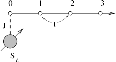
Figure 10: Illustrating the strong-coupling limit of the Kondo model

$$H_{lattice}=-t\sum_{j=0,\infty}[c{{}^{{\dagger}}}_{\sigma}(j+1)c_{\sigma}(j)+\hbox{H.c}]+Jc{{}^{{\dagger}}}_{\alpha}(0)\vec{\sigma}_{\alpha\beta}c_{\beta}(0)\cdot\vec{S_{d}}.$$ (87)

Nozières argued that the strong coupling fixed point will be described by the situation $J>>t$. In this limit, the kinetic energy of the electrons in the band can be treated as a perturbation to the Kondo singlet. The local moment couples to an electron at the origin, forming a “Kondo singlet” denoted by

$$|GS\rangle=\frac{1}{\sqrt{2}}\left(|\Uparrow\downarrow\rangle-|\Downarrow\uparrow\rangle\right)$$ (88)

where the thick arrow refers to the spin state of the local moment and the thin arrow refers to the spin state of the electron at site $0$. Any electron which migrates from site $1$ to site $0$ will automatically break this singlet state, raising its energy by $3J/4$. This will have the effect of excluding electrons (or holes) from the origin. The fixed point Hamiltonian must then take the form

$$H_{lattice}=-t\sum_{j=1,\infty}[c{{}^{{\dagger}}}_{\sigma}(j+1)c_{\sigma}(j)+\hbox{H.c}]+\hbox{weak interaction}$$ (89)

where the second-term refers to the weak-interactions induced in the conduction sea by virtual fluctuations onto site $0$. If the wavefunction of electrons far from the impurity has the form $\psi(x)\sim\sin(k_{F}x)$, where $k_{F}$ is the Fermi momentum, then the exclusion of electrons from site $1$ has the effect of phase-shifting the electron wavefunctions by one the lattice spacing $a$, so that now $\psi(x)\sim\sin(k_{F}x-\delta)$ where $\delta=k_{F}a$. But if there is one electron per site, then $2(2k_{F}a/(2\pi))=1$ by the Luttinger sum rule, so that $k_{F}=\pi/(2a)$ and hence the Kondo singlet acts as a spinless, elastic scattering center with scattering phase shift

$$\delta=\pi/2.$$ (90)

The appearance of $\delta=\pi/2$ could also be deduced by appealing to the Friedel sum rule, which states that the number of bound-electrons at the magnetic impurity site is $\sum_{\sigma}\frac{\delta_{\sigma=\pm 1}}{\pi}=2\delta/\pi$, so that $\delta=\pi/2$. By considering virtual fluctuations of electrons between site $1$ and $0$, Nozières argued that the induced interaction at site $1$ must take the form

$$H_{int}\sim\frac{t^{4}}{J^{3}}n_{1\uparrow}n_{1\downarrow}$$ (91)

because fourth order hopping processes lower the energy of the singly occupied state, but they do not occur for the doubly occupied state. This is a repulsive interaction amongst the conduction electrons, and it is known to be a marginal operator under the renormalization group, leading to the conclusion that the effective Hamiltonian describes a weakly interacting “local” Fermi liquid.

Nozières formulated this local Fermi liquid in the language of an occupancy-dependent phase shift. Suppose the $k\sigma$ scattering state has occupancy $n_{k\sigma}$, then the the ground-state energy will be a functional of these occupancies $E[\{n_{k\sigma}\}]$. The differential of this quantity with respect to occupancies defines a phase shift as follows

$$\frac{\delta E}{\delta n_{k\sigma}}=\epsilon_{k}-\frac{\Delta\epsilon}{\pi}{\delta(\{n_{k^{\prime}\sigma^{\prime}}\},\epsilon_{k})}.$$ (92)

The first term is just the energy of an unscattered conduction electron, while $\delta(\{n_{k^{\prime}\sigma^{\prime}}\},\epsilon_{k})$ is the scattering phase shift of the Fermi liquid. This phase shift can be expanded

$${\delta(\{n_{k^{\prime}\sigma^{\prime}}\},\epsilon_{k})}=\frac{\pi}{2}+\alpha(\epsilon_{k}-\mu)+\Phi\sum_{k}\delta n_{k,-\sigma}$$ (93)

where the term with coefficient $\Phi$ describes the interaction between opposite spin states of the Fermi liquid. Nozières argued that when the chemical potential of the conduction sea is changed, the occupancy of the localized $d$ state will not change, which implies that the phase shift is invariant under changes in $\mu$. Now under a shift $\delta\mu$, the change in the occupancy $\sum_{k}\delta n_{k\sigma}\rightarrow\delta\mu\rho$, so that changing the chemical potential modifies the phase shift by an amount

$$\Delta\delta=(\alpha+\Phi\rho)\Delta\mu=0$$ (94)

so that $\alpha=-\rho\Phi$. We are now in a position to calculate the impurity contribution to the magnetic susceptibility and specific heat. First note that the density of quasiparticle states is given by

$$\rho=\frac{dN}{dE}=\rho_{o}+\frac{1}{\pi}\frac{\partial\delta}{\partial\epsilon}=\rho_{o}+\frac{\alpha}{\pi}$$ (95)

so that the low temperature specific heat is given by $C_{V}=(\gamma_{bulk}+\gamma_{i})$ where

$$\gamma_{i}=2\left(\frac{\pi^{2}k_{B}^{2}}{3}\right)\frac{\alpha}{\pi}$$ (96)

where the prefactor “$2$” is derived from the spin up and spin-down bands. Now in a magnetic field, the impurity magnetization is given by

$$M=\frac{\delta_{\uparrow}}{\pi}-\frac{\delta_{\downarrow}}{\pi}$$ (97)

Since the Fermi energies of the up and down quasiparticles are shifted to $\epsilon_{F\sigma}\rightarrow\epsilon_{F}-\sigma B$, we have $\sum_{k}\delta n_{k\sigma}=\sigma\rho B$, so that the phase-shift at the Fermi surface in the up and down scattering channels becomes

$$\delta_{\sigma} = \frac{\pi}{2}+\alpha\delta\epsilon_{F\sigma}+\Phi(\sum_{k}\delta n_{k\sigma}$$ (98)

$$= \frac{\pi}{2}+\alpha\sigma B-\Phi\rho\sigma B$$ (99)

$$= \frac{\pi}{2}+2\alpha\sigma B$$ (100)

so that the presence of the interaction term doubles the size of the change in the phase shift due to a magnetic field. The impurity magnetization then becomes

$$M_{i}=\chi_{i}B=2\left(\frac{2\alpha}{\pi}\right)\mu_{B}^{2}B$$ (101)

where we have reinstated the magnetic moment of the electron. This is twice the value expected for a “rigid” resonance, and it means that the Wilson ratio is

$$W=\frac{\chi_{i}\pi^{2}k_{B}^{2}}{\gamma_{i}3(\mu_{B})^{2}}=2$$ (102)

2.7 Experimental observation of Kondo effect in real materials and quantum dots

Experimentally, there is now a wealth of observations that confirm our understanding of the single impurity Kondo effect. Here is a brief itemization of some of the most important observations. (Fig. 11.)

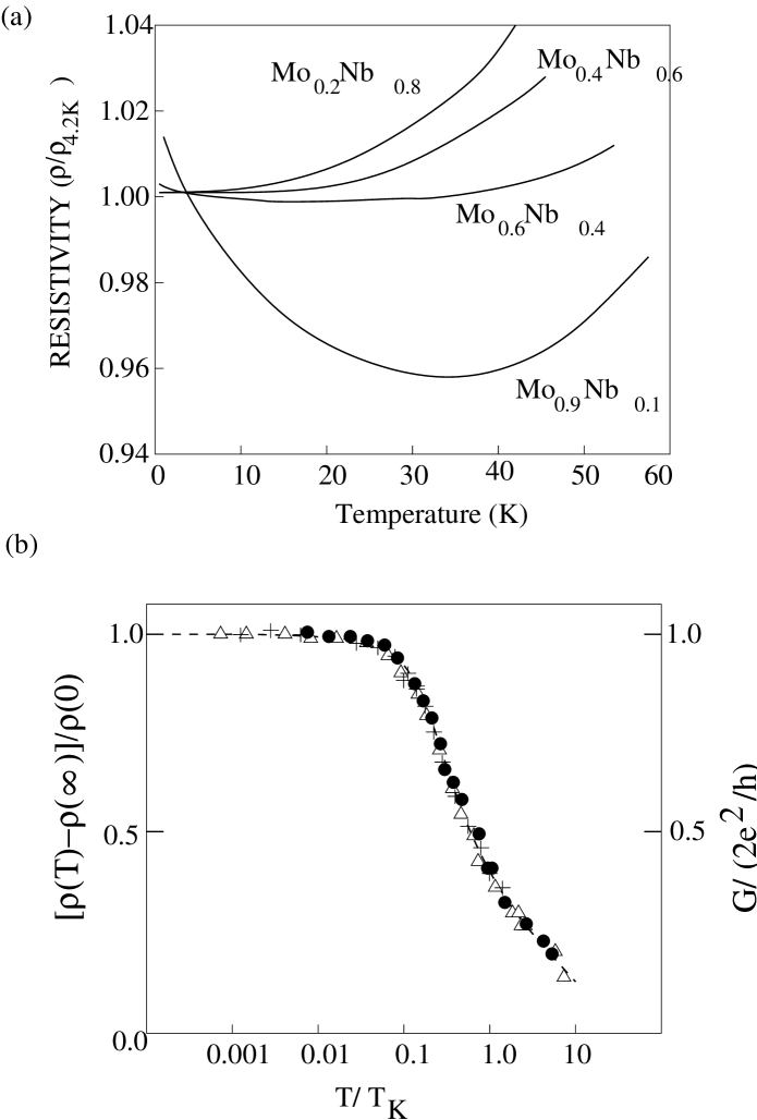
Figure 11: (a) Sketch of resistance minimum in $Mo_{x}Nb_{1-x}$ (b) Sketch of excess resistivity associated with scattering from an impurity spin. Right hand-scale- differential conductivity of a quantum dot.

• A resistance minimum appears when local moments develop in a material. For example, in $Nb_{1-x}Mo_{x}$ alloys, a local moment develops for $x>0.4$, and the resistance is seen to develop a minimum beyond this point.sarachik64 ; clogston62

• Universality seen in the specific heat $C_{V}=\frac{n_{i}}{T}F(T/T_{K})$ of metals doped with dilute concentrations of impurities. Thus the specific heat of $\underline{Cu}-Fe$ (iron impurities in copper) can be superimposed on the specific heat of $\underline{Cu}-Cr$, with a suitable rescaling of the temperature scale. white79 ; triplett70

• Universality is observed in the differential conductance of quantum dotsCronenwett:1998 ; vanderWiel:2000 and spin-fluctuation resistivity of metals with a dilute concentration of impurities.hedgcock63 Actually, both properties are dependent on the same thermal average of the imaginary part of the scattering T-matrix

  $$\rho_{i} = n_{i}\frac{ne^{2}}{m}\int d\omega\left(-\frac{\partial f}{\partial\omega}\right)2Im[T(\omega)]$$ (103)

  $$G = \frac{2e^{2}}{{\mathchar 22\relax\mkern-9.0muh}}\int d\omega\left(-\frac{\partial f}{\partial\omega}\right)\pi\rho Im[T(\omega)].$$ (104)

  Putting $\pi\rho\int d\omega\left(-\frac{\partial f}{\partial\omega}\right)\hbox{Im}T(\omega)=t(\omega/T_{K},T/T_{K})$, we see that both properties have the form

  $$\rho_{i} = n_{i}\frac{2ne^{2}}{\pi m\rho}t(T/T_{K})$$ (105)

  $$G = \frac{2e^{2}}{{\mathchar 22\relax\mkern-9.0muh}}t(T/T_{K})$$ (106)

  where $t(T/T_{K})$ is a universal function. This result is born out by experiment.

2.8 Exercises

1. Generalize the scaling equations to the anisotropic Kondo model with an anisotropic interaction

   $$H_{I}=\sum_{|\epsilon_{k}|,|\epsilon_{k^{\prime}},a=(x,y,z)}J^{a}c{{}^{{\dagger}}}_{k\alpha}{\sigma}^{a}_{\alpha\beta}c_{k^{\prime}\beta}\cdot{S^{a}}_{d}$$ (107)

   and show that the scaling equations take the form

   $$\frac{\partial J_{a}}{\partial\ln D}=-2J_{b}J_{c}\rho+O(J^{3}),$$

   where and $(a,b,c)$ are a cyclic permutation of $(x,y,z)$. Show that in the special case where $J_{x}=J_{y}=J_{\perp}$, the scaling equations become

   $$\frac{\partial J_{\perp}}{\partial\ln D} = -2J_{z}J_{\perp}\rho+O(J^{3}),$$ (108)

   $$\frac{\partial J_{z}}{\partial\ln D} = -2(J_{z})^{2}\rho+O(J^{3}),$$ (109)

   so that $J_{z}^{2}-J_{\perp}^{2}=\hbox{constant}$. Draw the corresponding scaling diagram.

2. Consider the symmetric Anderson model, with a symmetric band-structure at half filling. In this model, the $d^{0}$ and $d^{2}$ states are degenerate and there is the possibility of a “charged Kondo effect” when the interaction $U$ is negative. Show that under the “particle-hole” transformation

   $$c_{k\uparrow} \rightarrow c_{k\uparrow},\qquad d_{\uparrow}\rightarrow d_{\uparrow}$$ (110)

   $$c_{k\downarrow} \rightarrow -c{{}^{{\dagger}}}_{k\downarrow},\qquad d_{\downarrow}\rightarrow-d{{}^{{\dagger}}}_{\downarrow}$$ (111)

   the positive $U$ model is transformed to the negative $U$ model. Show that the spin operators of the local moment are transformed into Nambu “isospin operators” which describe the charge and pair degrees of freedom of the d-state. Use this transformation to argue that when U is negative, a charged Kondo effect will occur at exactly half-filling involving quantum fluctuations between the degenerate $d^{0}$ and $d^{2}$ configurations.

3. What happens to the Schrieffer-Wolff transformation in the infinite U limit? Rederive the Schrieffer-Wolff transformation for an N-fold degenerate version of the infinite U Anderson model. This is actually valid for Ce and Yb ions.

4. Rederive the Nozières Fermi liquid picture for an SU (N) degenerate Kondo model. Explain why this picture is relevant for magnetic rare earth ions such as $Ce^{3+}$ or $Yb^{3+}$.

5. Check the Popov trick works for a magnetic moment in an external field. Derive the partition function for a spin in a magnetic field using this method.

6. Use the Popov trick to calculate the T-matrix diagrams for the leading Kondo renormalization diagramatically.

3 Heavy Fermions

Although the single impurity Kondo problem was essentially solved by the early seventies, it took a further decade before the physics community was ready to accept the notion that the same phenomenon could occur within a dense lattice environment. This resistance to change was rooted in a number of popular misconceptions about the spin physics and the Kondo effect.

At the beginning of the seventies, it was well known that local magnetic moments severely suppress superconductivity, so that typically, a few percent is all that is required to destroy the superconductivity. Conventional superconductivity is largely immune to the effects of non-magnetic disorder but highly sensitive to magnetic impurities, which destroy the time-reversal symmetry necessary for s-wave pairing. The arrival of a new class of superconducting material containing dense arrays of local moments took the physics community completely by surprise. Indeed, the first observations of superconductivity in $UBe_{13}$, made in 1973 bucher were dismissed as an artifact and had to await a further ten years before they were revisited and acclaimed as heavy fermion superconductivity. steglich ; ott

Normally, local moment systems develop antiferromagnetic order at low temperatures. When a magnetic moment is introduced into a metal it induces Friedel oscillations in the spin density around the magnetic ion, given by

$$\langle\vec{M}(x)\rangle=-J\chi(\vec{x}-\vec{x}^{\prime})\langle\vec{S}(\vec{x}^{\prime})\rangle$$

where $J$ is the strength of the Kondo coupling and

$$\chi(x) = \sum_{\vec{q}}\chi(\vec{q})e^{i\vec{q}\cdot\vec{x}}$$ (112)

$$\chi(\vec{q}) = 2\sum_{\vec{k}}\frac{f(\epsilon_{\vec{k}})-f(\epsilon_{\vec{k}+\vec{q}})}{\epsilon_{\vec{k}+\vec{q}}-\epsilon_{\vec{k}}}$$ (113)

is the the non-local susceptibility of the metal.

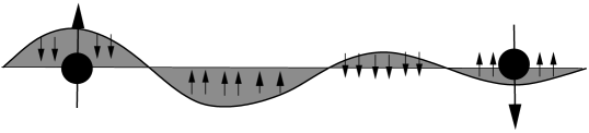
Figure 12: Illustrating how the polarization of spin around a magnetic impurity gives rise to Friedel oscillations and induces an RKKY interaction between the spins

If a second local moment is introduced at location $\vec{x}$, then it couples to $\langle M(\vec{x})\rangle$ giving rise to a long-range magnetic interaction called the “RKKY”rkky interaction,

$$H_{RKKY}=\overbrace{-J^{2}\chi(\vec{x}-\vec{x}^{\prime})}^{{J_{RKKY}(\vec{x}-\vec{x}^{\prime})}}\vec{S}(x)\cdot\vec{S}(x^{\prime}).$$ (114)

The sharp discontinuity in the occupancies at the Fermi surface produces slowly decaying Friedel oscillations in the RKKY interaction given by

$$J_{RKKY}(r)\sim-J^{2}\rho\frac{\cos 2k_{F}r}{|k_{F}r|^{3}}$$ (115)

where $\rho$ is the conduction electron density of states and $r$ is the distance from the impurity, so the RKKY interaction oscillates in sign, depending on the distance between impurities. The approximate size of the RKKY interaction is given by $E_{RKKY}\sim J^{2}\rho$.

Normally, the oscillatory nature of this magnetic interaction favors the development of antiferromagnetism. In alloys containing a dilute concentration of magnetic transition metal ions, the RKKY interaction gives rise to a frustrated, glassy magnetic state known as a spin glass in which the magnetic moments freeze into a fixed, but random orientation. In dense systems, the RKKY interaction typically gives rise to an ordered antiferromagnetic state with a Néel temperature $T_{N}\sim J^{2}\rho$.

In 1976 Andres, Ott and Graebner discovered the heavy fermion metal $CeAl_{3}$. ott76 This metal has the following features:

• A Curie susceptibility $\chi^{-1}\sim T$ at high temperatures.

• A paramagnetic spin susceptibility $\chi\sim constant$ at low temperatures.

• A linear specific heat capacity $C_{V}=\gamma T$, where $\gamma\sim 1600mJ/mol/K^{2}$ is approximately $1600$ times larger than in a conventional metal.

• A quadratic temperature dependence of the low temperature resistivity $\rho=\rho_{o}+AT^{2}$

Andres, Ott and Grabner pointed out that the low temperature properties are those of a Fermi liquid, but one in which the effective masses of the quasiparticles are approximately $1000$ larger than the bare electron mass. The Fermi liquid expressions for the magnetic susceptibility $\chi$ and the linear specific heat coefficient $\gamma$ are

$$\chi = (\mu_{B})^{2}\frac{N^{*}(0)}{1+F_{o}^{a}}$$ (116)

$$\gamma = \frac{\pi^{2}k_{B}^{2}}{3}N^{*}(0)$$ (117)

where $N^{*}(0)=\frac{m^{*}}{m}N(0)$ is the renormalized density of states and $F_{0}^{a}$ is the spin-dependent part of the s-wave interaction between quasiparticles. What could be the origin of this huge mass renormalization? Like other Cerium heavy fermion materials, the Cerium atoms in this metal are in a $Ce^{3+}(4f^{1})$ configuration, and because they are spin-orbit coupled, they form huge local moments with a spin of $J=5/2$. In their paper, Andres, Ott and Graebner suggested that a lattice version of the Kondo effect might be responsible.

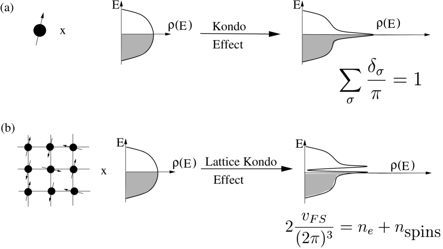
Figure 13: (a) Single impurity Kondo effect builds a single fermionic level into the conduction sea, which gives rise to a resonance in the conduction electron density of states (b) Lattice Kondo effect builds a fermionic resonance into the conduction sea in each unit cell. The elastic scattering off this lattice of resonances leads to formation of a heavy electron band, of width $T_{K}$.

This discovery prompted Sebastian Doniachdoniach78 to propose that the origin of these heavy electrons derived from a dense version of the Kondo effect. Doniach proposed that heavy electron systems should be modeled by the “Kondo-lattice Hamiltonian” where a dense array of local moments interact with the conduction sea. For a Kondo lattice with spin $1/2$ local moments, the Kondo lattice Hamiltoniankasuya52 takes the form

$$H=\sum_{\vec{k}\sigma}\epsilon_{\vec{k}}c{{}^{{\dagger}}}_{\vec{k}\sigma}c_{\vec{k}\sigma}+J\sum_{j}\vec{S}_{j}\cdot c{{}^{{\dagger}}}_{\vec{k}\alpha}\left(\frac{\vec{\sigma}}{2}\right)_{\alpha\beta}c_{\vec{k}^{\prime}\beta}e^{i(\vec{k}^{\prime}-\vec{k})\cdot\vec{R}_{j}}$$ (118)

Doniach argued that there are two scales in the Kondo lattice, the Kondo temperature $T_{K}$ and $E_{RKKY}$, given by

$$T_{K} = De^{-1/2J\rho}$$ (119)

$$E_{RKKY} = J^{2}\rho$$ (120)

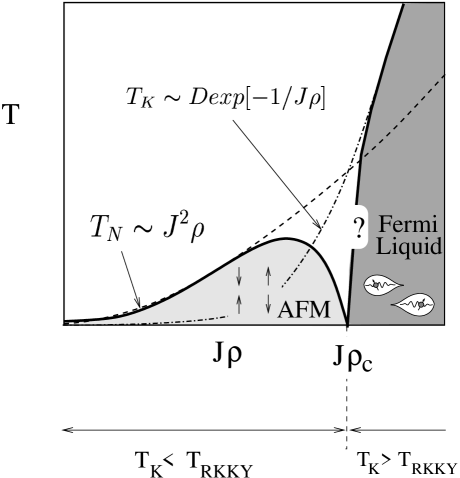
Figure 14: Doniach diagram, illustrating the antiferromagnetic regime, where $T_{K}<T_{RKKY}$ and the heavy fermion regime, where $T_{K}>T_{RKKY}$. Experiment has told us in recent times that the transition between these two regimes is a quantum critical point. The effective Fermi temperature of the heavy Fermi liquid is indicated as a solid line. Circumstantial experimental evidence suggests that this scale drops to zero at the antiferromagnetic quantum critical point, but this is still a matter of controversy.

When $J\rho$ is small, then $E_{RKKY}>>T_{K}$, and an antiferromagnetic state is formed, but when the Kondo temperature is larger than the RKKY interaction scale, $T_{K}>>E_{RKKY}$, Doniach argued that a dense Kondo lattice ground-state is formed in which each site resonantly scatters electrons. Bloch’s theorem then insures that the resonant elastic scattering at each site will form a highly renormalized band, of width $\sim T_{K}$. By contrast to the single impurity Kondo effect, in the heavy electron phase of the Kondo lattice the strong elastic scattering at each site acts in a coherent fashion, and does not give rise to a resistance. For this reason, as the heavy electron state forms, the resistance of the system drops towards zero.

Figure 15: Development of coherence in heavy fermion systems. Resistance in $Ce_{1-x}La_{x}Cu_{6}$ after Onuki and Komatsubaraonuki87

One of the fascinating aspects of the Kondo lattice concerns the Luttinger sum rule. This aspect was first discussed in detail by Martinmartin82 , who pointed out that the Kondo model can be regarded as the result of adiabatically increasing the interaction strength $U$ in the Anderson model, whilst preserving the valence of the magnetic ion. During this process, one expects sum rules to be preserved. In the impurity, the scattering phase shift at the Fermi energy counts the number of localized electrons, according to the Friedel sum rule

$$\sum_{\sigma}\frac{\delta_{\sigma}}{\pi}=n_{f}=1$$

This sum rule survives to large $U$, and reappears as the constraint on the scattering phase shift created by the Abrikosov Suhl resonance. In the lattice, the corresponding sum rule is the Luttinger sum rule, which states that the Fermi surface volume counts the number of electrons, which at small $U$ is just the number of localized (4f, 5f or 3d) and conduction electrons. When $U$ becomes large, number of localized electrons is now the number of spins, so that

$$2\frac{{\cal V}_{FS}}{(2\pi)^{3}}=n_{e}+n_{\hbox{spins}}$$

This sum rule is thought to hold for the Kondo lattice Hamiltonian, independently of the origin of the localized moments. Such a sum rule would work, for example, even if the spins in the model were derived from nuclear spins, provided the Kondo temperature were large enough to guarantee a paramagnetic state.

Experimentally, there is a great deal of support for the above picture. It is possible, for example, to examine the effect of progressively increasing the concentration of $Ce$ in the non-magnetic host $LaCu_{6}$.(15 ) At dilute concentrations, the resistivity rises to a maximum at low temperatures. At dense concentrations, the resistivity shows the same high temperature behavior, but at low temperatures coherence between the sites leads to a dramatic drop in the resistivity. The thermodynamics of the dense and dilute system are essentially identical, but the transport properties display the effects of coherence.

There are also indications that the Fermi surface of heavy electron systems does have the volume which counts both spins and conduction electrons, derived from Fermi surface studies. lonzarich1 ; lonzarich2

3.1 Some difficulties to overcome.

The Doniach scenario for heavy fermion development is purely a comparison of energy scales: it does not tell us how the heavy fermion phase evolves from the antiferromagnet. There were two early objections to Doniach’s idea:

• Size of the Kondo temperature $T_{K}$. Simple estimates of the value of $J\rho$ required for heavy electron behavior give a value $J\rho\sim 1$. Yet in the Anderson model, $J\rho\sim 1$ would imply a mixed valent situation, with no local moment formation.

• Exhaustion paradox. The naive picture of the Kondo model imagines that the local moment is screened by conduction electrons within an energy range $T_{K}$ of the Fermi energy. The number of conduction electrons in this range is of order $T_{K}/D<<1$ per unit cell, where $D$ is the band-width of the conduction electrons, suggesting that there are not enough conduction electrons to screen the local moments.

The resolution of these two issues are quite intriguing.

3.1.1 Enhancement of the Kondo temperature by spin degeneracy

The resolution of the first issue has its origins in the large spin-orbit coupling of the rare earth or actinide ions in heavy electron systems. This protects the orbital angular momentum against quenching by the crystal fields. Rare earth and actinide ions consequently display a large total angular momentum degeneracy $N=2j+1$, which has the effect of dramatically enhancing the Kondo temperature. Take for example the case of the Cerium ion, where the $4f^{1}$ electron is spin-orbit coupled into a state with $j=5/2$, giving a spin degeneracy of $N=2j+1=6$. Ytterbium heavy fermion materials involve the $Yb:4f^{13}$ configuration, which has an angular momentum $j=7/2$, or $N=8$.

To take account of these large spin degeneracies, we need to generalize the Kondo model. This was done in the mid-sixties by Coqblin and Schrieffercoqblin . Coqblin and Schrieffer considered a degenerate version of the infinite $U$ Anderson model in which the spin component of the electrons runs from $-j$ to $j$,

$$H=\sum_{{k}\sigma}\epsilon_{{k}}c{{}^{{\dagger}}}_{{k}\sigma}c_{{k}\sigma}+E_{f}\sum_{\sigma}|f^{1}:\sigma\rangle\langle f^{1}:\sigma|+\sum_{k,\sigma}V\left[c{{}^{{\dagger}}}_{{k}\sigma}|f^{0}\rangle\langle f^{1}:\sigma|+\hbox{H.c.}\right].$$

Here the conduction electron states are also labeled by spin indices that run from $-j$ to $j$. This is because the spin-orbit coupled $f$ states couple to partial wave states of the conduction electrons in which the orbital and spin angular momentum are combined into a state of definite $j$. Suppose $|\vec{k}\sigma\rangle$ represents a plane wave of momentum $\vec{k}$, then one can construct a state of definite orbital angular momentum $l$ by integrating the plane wave with a spherical harmonic, as follows:

$$|klm\sigma\rangle=\int\frac{d\Omega}{4\pi}|\vec{k}\sigma\rangle Y^{*}_{lm}(\hat{k})$$

When spin orbit interactions are strong, one must work with a partial wave of definite $j$, obtained by combining these states in the following linear combinations. Thus for the case $j=l+1/2$ (relevant for Ytterbium ions), we have

$$|km\rangle=\sum_{\sigma=\pm 1}\sqrt{\frac{l+\sigma m+\frac{1}{2}}{2l+1}}|klm-\frac{\sigma}{2},\frac{\sigma}{2}\rangle.$$

An electron creation operator is constructed in a similar way. This construction is unfortunately, not simultaneously possible at more than one site.

When $E_{f}<<0$, the valence of the ion approaches unity and $n_{f}\rightarrow 1$. In this limit, one can integrate out the virtual fluctuations $f^{1}\rightleftharpoons f^{0}+e^{-}$ via a Schrieffer Wolff transformation. This leads to the Coqblin Schrieffer model

$$H_{CS}=\sum_{{k}\sigma}\epsilon_{{k}}c{{}^{{\dagger}}}_{{k}\sigma}c_{{k}\sigma}+J\sum_{k,k^{\prime},\alpha\beta}c{{}^{{\dagger}}}_{k\beta}c_{{k^{\prime}}\alpha}\Gamma_{\alpha\beta},\qquad(\sigma,\alpha,\beta\in[-j,j]).$$

where $J=V^{2}/|E_{f}|$ is the induced antiferromagnetic interaction strength. This interaction is understood as the result of virtual charge fluctuations into the $f^{0}$ state, $f^{1}\rightleftharpoons f^{0}+e^{-}$. The spin indices run from $-j$ to $j$, and we have introduced the notation

$$\Gamma_{\alpha\beta}\equiv f{{}^{{\dagger}}}_{\alpha}f_{\beta}=|f^{1}:\alpha\rangle\langle f^{1}:\beta|$$

Notice that the charge $Q=n_{f}$ of the $f-$electron, normally taken to be unity, is conserved by the spin-exchange interaction in this Hamiltonian.

To get an idea of how the Kondo effect is modified by the larger degeneracy, consider the renormalization of the interaction, which is given by the diagram

$$J_{eff}(D^{\prime}) =$$ (121)

$$= J+NJ^{2}\rho\ln\left(\frac{D}{D^{\prime}}\right)$$ (123)

( where the cross on the intermediate conduction electron state indicates that all states with energy $|\epsilon_{k}|\in[D^{\prime},D]$ are integrate over). From this result, we see that $\beta(g)=\partial g(D)/\partial\ln D=-Ng^{2}$, where $g=J\rho$ has an $N-$ fold enhancement, derived from the $N$ intermediate hole states. A more extensive calculation shows that the beta function to third order takes the form

$$\beta(g)=-Ng^{2}+Ng^{3}.$$ (124)

This then leads to the Kondo temperature

$$T_{K}=D(NJ\rho)^{\frac{1}{N}}\exp\left[-\frac{1}{NJ\rho}\right]$$

so that large degeneracy enhances the Kondo temperature in the exponential factor. By contrast, the RKKY interaction strength is given by $T_{RKKY}\sim J^{2}\rho$, and it does not involve any $N$ fold enhancement factors, thus in systems with large spin degeneracy, the enhancement of the Kondo temperature favors the formation of the heavy fermion ground-state.

In practice, rare-earth ions are exposed to the crystal fields of their host, which splits the $N=2j+1$ fold degeneracy into many multiplets. Even in this case, the large degeneracy is helpful, because the crystal field splitting is small compared with the band-width. At energies $D^{\prime}$ large compared with the crystal field splitting $T_{x}$, $D^{\prime}>>T_{x}$, the physics is that of an $N$ fold degenerate ion, whereas at energies $D^{\prime}$ small compared with the crystal field splitting, the physics is typically that of a Kramers doublet, i.e.

(125)

(126)

$$\frac{\partial g}{\partial\ln D} = \left\{\begin{array}[]{lr}-Ng^{2}&(D>>T_{x})\cr-2g^{2}&(D<<T_{x})\end{array}\right.$$ (129)

from which we see that at low energy scales, the leading order renormalization of $g$ is given by

$$\frac{1}{g(D^{\prime})}=\frac{1}{g_{o}}-N\ln\left(\frac{D}{T_{x}}\right)-2\ln\left(\frac{T_{x}}{D^{\prime}}\right)$$

where the first logarithm describes the high energy screening with spin degeneracy $N$, and the second logarithm describes the low-energy screening, with spin degeneracy 2. This expression is $\sim 0$ when $D^{\prime}\sim T_{K}^{*}$, the Kondo temperature, so that

$$0=\frac{1}{g_{o}}-N\ln\left(\frac{D}{T_{x}}\right)-2\ln\left(\frac{T_{x}}{T^{*}_{K}}\right)$$

from which we deduce that the renormalized Kondo temperature has the formsato

$$T_{K}^{*}=D\exp\left(-\frac{1}{2J_{o}\rho}\right)\left(\frac{D}{T_{x}}\right)^{\frac{N}{2}-1}.$$

Here the first term is the expression for the Kondo temperature of a spin $1/2$ Kondo model. The second term captures the enhancement of the Kondo temperature coming from the renormalization effects at scales larger than the crystal field splitting. Suppose $T_{x}\sim 100K$, and $D\sim 1000K$, and $N=6$, then the enhancement factor is order $100$. This effect enhances the Kondo temperature of rare earth heavy fermion systems to values that are indeed, up to a hundred times bigger than those in transition metal systems. This is the simple reason why heavy fermion behavior is rare in transition metal systems. takagi In short- spin-orbit coupling, even in the presence of crystal fields, substantially enhances the Kondo temperature.

3.1.2 The exhaustion problem

At temperatures $T{{\lower 4.0pt\hbox{$<$}}\atop\widetilde{\ \ \ }}T_{K}$, a local moment is “screened” by conduction electrons. What does this actually mean? The conventional view of the Kondo effect interprets it in terms of the formation of a “magnetic screening cloud” around the local moment. According to the screening cloud picture, the electrons which magnetically screen each local moment are confined within an energy range of order $\delta\epsilon\sim T_{K}$ around the Fermi surface, giving rise to a spatially extended screening cloud of dimension ${l}=v_{F}/T_{K}\sim a\frac{\epsilon_{F}}{T_{K}}$, where $a$ is a lattice constant and $\epsilon_{F}$ is the Fermi temperature. In a typical heavy fermion system, this length would extend over hundreds of lattice constants. This leads to the following two dilemmas

1. It suggests that when the density of magnetic ions is greater than $\rho\sim 1/l^{3}$, the screening clouds will interfere. Experimentally no such interference is observed, and features of single ion Kondo behavior are seen at much higher densities.

2. “ The exhaustion paradox” The number of “screening”electrons per unit cell within energy $T_{K}$ of the Fermi surface roughly $T_{K}/W$, where $W$ is the bandwidth, so there would never be enough low energy electrons to screen a dense array of local moments.

In this lecture I shall argue that the screening cloud picture of the Kondo effect is conceptually incorrect. Although the Kondo effect does involve a binding of local moments to electrons, the binding process takes place between the local moment and high energy electrons , spanning decades of energy from the Kondo temperature up to the band-width. (Fig. 16) I shall argue that the key physics of the Kondo effect, both in the dilute impurity and dense Kondo lattice, involves the formation of a composite heavy fermion formed by binding electrons on logarithmically large energy scales out to the band-width.

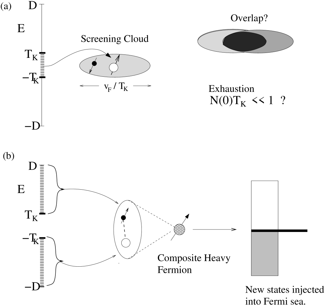
Figure 16: Contrasting (a) the “screening cloud” picture of the Kondo effect with (b) the composite fermion picture. In (a), low energy electrons form the Kondo singlet, leading to the exhaustion problem. In (b) the composite heavy electron is a highly localized bound-state between local moments and high energy electrons which injects new electronic states into the conduction sea at the chemical potential. Hybridization of these states with conduction electrons produces a singlet ground-state, forming a Kondo resonance in the single impurity, and a coherent heavy electron band in the Kondo lattice.

These new electronic states are injected into the conduction electron sea near the Fermi energy. For a single impurity, this leads to a single isolated resonance. In the lattice, the presence of a new multiplet of fermionic states at each site leads to the formation of a coherent heavy electron band with an expanded Fermi surface. ( 16)

3.2 Large N Approach

We shall now solve the Kondo model, both the single impurity and the lattice, in the large $N$ limit. In the early eighties, AndersonandersonlargeN pointed out that the large spin degeneracy $N=2j+1$ furnishes a small parameter $1/N$ which might be used to develop a controlled expansion about the limit $N\rightarrow\infty$. Anderson’s observation immediately provided a new tool for examining the heavy fermion problem: the so called “large $N$ expansion”. witten .

The basic idea behind the large $N$ expansion, is to take a limit where every term in the Hamiltonian grows extensively with $N$. In this limit, quantum fluctuations in intensive variables, such as the electron density, become smaller and smaller, scaling as $1/N$, and in this sense,

$$\frac{1}{N}\sim{\mathchar 22\relax\mkern-9.0muh}_{eff}$$

behaves as an effective Planck’s constant for the theory. In this sense, a large $N$ expansion is a semi-classical treatment of the quantum mechanics, but instead of expanding around ${\mathchar 22\relax\mkern-9.0muh}=0$, one can obtain new, non trivial results by expanding around the non trivial solvable limit $\frac{1}{N}=0$. For the Kondo model, we are lucky, because the important physics of the Kondo effect is already captured by the large $N$ limit as we shall now see.

Our model for a Kondo lattice or an ensemble of Kondo impurities localized at sites $j$ is

$$H=\sum_{\vec{k}\sigma}\epsilon_{\vec{k}}c{{}^{{\dagger}}}_{\vec{k}\sigma}c_{\vec{k}\sigma}+\sum_{j}H_{I}(j)$$ (130)

where

$$H_{I}(j)=\frac{J}{N}\Gamma_{\alpha\beta}(j)\psi{{}^{{\dagger}}}_{\beta}(j)\psi_{\alpha}(j)$$

is the interaction Hamiltonian between the local moment and conduction sea. Here, the spin of the local moment at site $j$ is represented using pseudo-fermions

$$\Gamma_{\alpha\beta}(j)=f{{}^{{\dagger}}}_{j\alpha}f_{j\beta},$$

and

$$\psi{{}^{{\dagger}}}_{\alpha}(j)=\sum_{\vec{k}}c{{}^{{\dagger}}}_{\vec{k}\alpha}e^{-i\vec{k}\cdot\vec{R}_{j}}$$

creates an electron localized at site $j$.

There are a number of technical points about this model that need to be discussed:

• The spherical cow approximation. For simplicity, we assume that electrons have a spin degeneracy $N=2j+1$. This is a theorists’ idealization- a “spherical cow approximation” which can only be strictly justified for a single impurity. Nevertheless, the basic properties of this toy model allow us to understand how the Kondo effect works in a Kondo lattice. With an $N$-fold conduction electron degeneracy, it is clear that the Kinetic energy will grow as $O(N)$.

• Scaling the interaction. Now the interaction part of the Hamiltonian $H_{I}(j)$ involves two sums over the spin variables, giving rise to a contribution that scales as $O(N^{2})$. To ensure that the interaction energy grows extensively with $N$, we need to scale the coupling constant as $O(1/N)$.

• Constraint $n_{f}=Q$. Irreducible representations of the rotation group SU (N) require that the number of $f-$electrons at a given site is constrained to equal to $n_{f}=Q$. In the large $N$ limit, it is sufficient to apply this constraint on the average $\langle n_{f}\rangle=Q$, though at finite $N$ a time dependent Lagrange multiplier coupled to the difference $n_{f}-Q$ is required to enforce the constraint dynamically. With $Q$ $f-$electrons, the spin operators $\Gamma_{ab}=f{{}^{{\dagger}}}_{a}f_{b}$ provide an irreducible antisymmetric representation of $SU(N)$ that is described by column Young Tableau with $Q$ boxes. As $N$ is made large, we need to ensure that $q=Q/N$ remains fixed, so that $Q\sim O(N)$ is an extensive variable. Thus, for instance, if we are interested in $N=2$, this corresponds to $q=n_{f}/N=\frac{1}{2}$. We may obtain insight into this case by considering the large $N$ limit with $q=1/2$.

The next step in the large $N$ limit is to carry out a “Hubbard Stratonovich” transformation on the interaction. We first write

$$H_{I}(j)=-\frac{J}{N}\left(\psi{{}^{{\dagger}}}_{j\beta}f_{j\beta}\right)\left(f{{}^{{\dagger}}}_{j\alpha}\psi_{j\alpha}\right),$$

with a summation convention on the spin indices. We now factorize thislacroix ; read as

$$H_{I}(j)\rightarrow H_{I}[V,j]=\bar{V}_{j}\left(\psi{{}^{{\dagger}}}_{j\alpha}f_{j\alpha}\right)+\left(f{{}^{{\dagger}}}_{j\alpha}\psi_{j\alpha}\right)V_{j}+N\frac{\bar{V}_{j}V_{j}}{J}$$

This is an exact transformation, provided the hybridization variables $V_{j}(\tau)$ are regarded as fluctuating variables inside a path integral, so formally,

$$Z=\int{\mathcal{D}}[V,\lambda]\overbrace{{\rm Tr}[T\exp\left[{-\int_{0}^{\beta}H[V,\lambda]}\right]]}^{Z[\lambda,V]}$$ (131)

where

$$H[V,\lambda]=\sum_{\vec{k}\sigma}\epsilon_{\vec{k}}c{{}^{{\dagger}}}_{\vec{k}\sigma}c_{\vec{k}\sigma}+\sum_{j}\left(H_{I}[V_{j},j]+\lambda_{j}[n_{f}(j)-Q]\right),$$ (132)

is exact. In this expression, ${\mathcal{D}}[V,\lambda]$ denotes a path integral over all possible time-dependences of $V_{j}$ and $\lambda_{j}(\tau)$, and $T$ denotes time ordering. The important point for our discussion here however, is that in the large $N$ limit, the Hamiltonian entering into this path integral grows extensively with $N$, so that we may write the partition function in the form

$$Z = \int{\mathcal{D}}[V,\lambda]{\rm Tr}[T\exp\left[{-N\int_{0}^{\beta}{\mathcal{H}}[V,\lambda]}\right]$$ (133)

where ${\mathcal{H}}[V,\lambda]=\frac{1}{N}H[V,\lambda]\sim O(1)$ is an intensive variable in $N$. The appearance of a large factor $N$ in the exponential means that this path integral becomes dominated by its saddle points in the large $N$ limit- i.e, if we choose

$$V_{j}=V_{o},\qquad\lambda_{j}=\lambda_{o}$$

where the saddle point values $V_{o}$ and $\lambda_{o}$ are chosen so that

$$\left.\frac{\partial\ln Z[V,\lambda]}{\partial V}\right|_{V_{j}=V_{o},\lambda_{j}=\lambda_{o}}=\left.\frac{\partial\ln Z[V,\lambda]}{\partial\lambda}\right|_{V_{j}=V_{o},\lambda_{j}=\lambda_{o}}=0$$

then in the large $N$ limit,

$$Z={\rm Tr}e^{-\beta H[V_{o},\lambda_{o}]}$$

In this way, we have converted the problem to a mean-field theory, in which the fluctuating variables $V_{j}(\tau)$ and $\lambda_{j}(\tau)$ are replaced by their saddle-point values. Our mean-field Hamiltonian is then

$$H_{MFT}=\sum_{\vec{k}\sigma}\epsilon_{\vec{k}}c{{}^{{\dagger}}}_{\vec{k}\sigma}c_{\vec{k}\sigma}+\sum_{j,\alpha}\left(f{{}^{{\dagger}}}_{j\alpha}\psi_{j\alpha}V_{o}+\bar{V}_{o}\psi{{}^{{\dagger}}}_{j\beta}f_{j\beta}+\lambda_{o}f{{}^{{\dagger}}}_{j\alpha}f_{j\alpha}\right)+Nn\left(\frac{\bar{V}_{o}V_{o}}{J}-\lambda_{o}q\right),$$

where n is the number of sites in the lattice. We shall now illustrate the use of this mean-field theory in two cases- the Kondo impurity, and the Kondo lattice. In the former, there is just one site; in the latter, translational invariance permits us to set $V_{j}=V_{o}$ at every site, and for convenience we shall choose this value to be real.

3.3 Mean-field theory of the Kondo impurity

3.3.1 Diagonalization of MF Hamiltonian

The Kondo effect is at heart, the formation of a many body resonance. To understand this phenomenon at its conceptually simplest, we begin with the impurity model. We shall begin by writing down the mean-field Hamiltonian for a single Kondo ion

$$H=\sum_{k\sigma}\epsilon_{k}c{{}^{{\dagger}}}_{k\sigma}c_{k\sigma}+\sum_{k\sigma}V[c{{}^{{\dagger}}}_{k\sigma}f_{\sigma}+f{{}^{{\dagger}}}_{\sigma}c_{k\sigma}]+\lambda\sum_{\sigma}n_{f\sigma}-\lambda Q+\frac{NV^{2}}{J}$$ (134)

By making a mean-field approximation, we have reduced the problem to one of a self-consistently determined resonant level model. Now, suppose we diagonalize this Hamiltonian, writing it in the form

$$H=\sum_{\gamma\sigma}E_{\gamma}a{{}^{{\dagger}}}_{\gamma\sigma}a_{\gamma\sigma}+\frac{NV^{2}}{J}-\lambda Q$$ (135)

where the “quasiparticle operators” $\alpha_{\gamma}$ are related via a unitary transformation to the original operators

$$a{{}^{{\dagger}}}_{\gamma\sigma}=\sum_{k}\alpha_{k}c{{}^{{\dagger}}}_{k\sigma}+\beta f{{}^{{\dagger}}}_{\sigma}.$$ (136)

commuting $a{{}^{{\dagger}}}_{\gamma\sigma}$ with $H$, we obtain

$$[H,\ a{{}^{{\dagger}}}_{\gamma\sigma}]=E_{\gamma}a{{}^{{\dagger}}}$$ (137)

Expanding the right and left-hand side of (137) in terms of (136) and (134), we obtain,

$$(E_{\gamma}-\epsilon_{k})\alpha_{k}-V\beta = 0$$ (138)

$$-V\sum_{k}\alpha_{k}+(E_{\gamma}-\lambda)\beta = 0$$ (139)

Solving for $\alpha_{k}$ using the first equation, and substituting into the second equation, we obtain

$$E_{\gamma}-\lambda-\sum_{k}\frac{V^{2}}{E_{\gamma}-\epsilon_{k}}=0$$ (140)

We could have equally well obtained these eigenvalue equations by noting the electron eigenvalues $E_{\gamma}$ must correspond to the poles of the f-Green function, $G_{f}(E_{\gamma})^{-1}=0$, where from an earlier subsection,

$$G_{f}^{-1}(\omega)=\left[\omega-\lambda-\sum_{k}\frac{V^{2}}{\omega-\epsilon_{k}}\right]$$ (141)

Either way, the one-particle excitation energies $E_{\gamma}$ must satisfy

$$E_{\gamma}=\lambda+\sum_{k}\frac{V_{o}^{2}}{E_{\gamma}-\epsilon_{k}}$$ (142)

The solutions of this eigenvalue equation are illustrated graphically in Fig. (17).

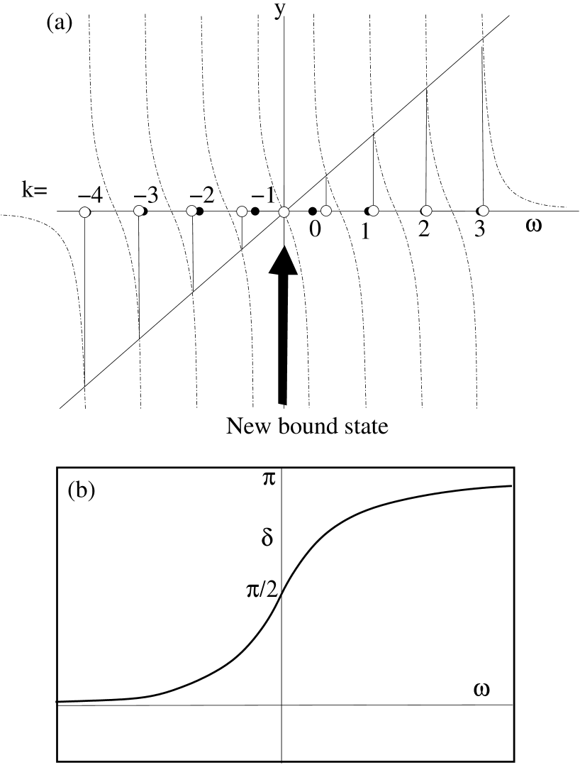
Figure 17: (a)Graphical solution of the equation $y=-\sum_{k}\frac{V^{2}}{y-\epsilon_{k}}$, for eight equally spaced conduction electron energies. Notice how the introduction of a new bound-state at $y=0$ displaces electron band-states both up and down in energy. In this way, the Kondo effect injects new bound-state fermion states into the conduction sea. (b) Energy dependence of the scattering phase shift.

Suppose the energies of the conduction sea are given by the $2M$ discrete values

$$\epsilon_{k}=(k+\frac{1}{2})\Delta\epsilon,\qquad k\in\{-M,\dots,M-1\}$$

Suppose we restrict our attention to the particle-hole case when the f-state is exactly half filled, i.e. when $Q=N/2$. In this situation, $\lambda=0$. We see that one solution to the eigenvalue equation corresponds to $E_{\gamma}=0$. The original band-electron energies are now displaced to both lower and higher energies, forming a band of $2M+1$ eigenvalues. Clearly, the effect of the hybridization is to inject one new fermionic eigenstate into the band. Notice however, that the electron states are displaced symmetrically either-side of the new bound-state at $E_{\gamma}=0$.

Each new eigenvalue is shifted relative to the original conduction electron energy by an amount of order $\Delta\epsilon$. Let us write

$$E_{\gamma}=\epsilon_{\gamma}-\Delta\epsilon\frac{\delta_{\gamma}}{\pi}$$

where $\delta\in[0,\pi]$ is called the “phase shift”. Substituting this into the eigenvalue equation, we obtain

$$E_{\gamma}=\lambda+\sum_{n=\gamma+1-M}^{{\gamma+M}}\frac{V_{o}^{2}}{\Delta\epsilon(n-\frac{\delta}{\pi})}$$

Now if $M$ is large, we can replace the sum over states in the above equation by an unbounded sum

$$E_{\gamma}=\lambda+\frac{V_{o}^{2}}{\Delta\epsilon}\sum_{n=-\infty}^{\infty}\frac{1}{(n-\frac{\delta}{\pi})}$$

Using contour integration methods, one can readily show that

$$\sum_{n=-\infty}^{{\infty}}\frac{1}{(n-\frac{\delta}{\pi})}=-\pi\cot\delta$$

so that the phase shift is given by $\delta_{\gamma}=\delta(E_{\gamma})$, where

$$\tan\delta[\epsilon]=\frac{\pi\rho V_{o}^{2}}{\lambda-\epsilon}$$

where we have replaced $\rho=\frac{1}{\Delta\epsilon}$ as the density of conduction electron states. This can also be written

$$\delta(\epsilon)=\tan^{-1}\left[\frac{\Delta}{\lambda-\epsilon}\right]={\rm Im}\ln[\lambda+i\Delta-\epsilon]$$ (143)

where $\Delta=\pi\rho V_{o}^{2}$ is the width of the resonant level induced by the Kondo effect. Notice that for $\lambda=0$, $\delta=\pi/2$ at the Fermi energy.

• The phase shift varies from $\delta=0$ at $E_{\gamma}=-\infty$ to $\delta=\pi$ at $E_{\gamma}=\infty$ , passing through $\delta=\pi/2$ at the Fermi energy.

• An extra state has been inserted into the band, squeezing the original electron states both down and up in energy to accommodate the additional state: states beneath the Fermi sea are pushed downwards, whereas states above the Fermi energy are pushed upwards. From the relation

  $$E_{\gamma}=\epsilon_{\gamma}-\frac{\Delta\epsilon}{\pi}\delta(E_{\gamma})$$

  we deduce that

  $$\frac{d\epsilon}{dE} = 1+\frac{\Delta\epsilon}{\pi}\frac{d\delta(E)}{dE}$$ (144)

  $$= 1+\frac{1}{\pi\rho}\frac{d\delta(E)}{dE}$$ (145)

  where $\rho=1/\Delta\epsilon$ is the density of states in the continuum. The new density of states $\rho^{*}(E)$is given by $\rho^{*}(E)dE=\rho d\epsilon$, so that

  $$\rho^{*}(E)=\rho(0)\frac{d\epsilon}{dE}=\rho+\rho_{i}(E)$$ (146)

  where

  $$\rho_{i}(E)=\frac{1}{\pi}\frac{d\delta(E)}{dE}=\frac{1}{\pi}\frac{\Delta}{(E-\lambda)^{2}+\Delta^{2}}$$ (147)

  corresponds to the enhancement of the conduction electron density of states due to injection of resonant bound-state.

3.3.2 Minimization of Free energy

With these results, let us now calculate the Free energy and minimize it to self-consistently evaluate $\lambda$ and $\Delta$. The Free energy is given by

$$F=-NT\sum_{\gamma}\ln[1+e^{-\beta E_{\gamma}}]-\lambda Q+\frac{NV_{o}^{2}}{J}.$$ (148)

In the continuum limit, where $\epsilon\rightarrow 0$, we can use the relation $E_{\gamma}=\epsilon_{\gamma}-\Delta\epsilon\frac{\delta}{\pi}$ to write

$$-T\ln[1+e^{-\beta E_{\gamma}}] = -T\ln[1+e^{-\beta(\epsilon_{\gamma}-\Delta\epsilon\frac{\delta}{\pi})}]$$ (149)

$$= \overbrace{-T\ln[1+e^{-\beta\epsilon_{\gamma}}]}^{{\rightarrow F_{0}}}-\frac{\Delta\epsilon}{\pi}{\delta(\epsilon_{\gamma})}f(\epsilon_{\gamma})$$ (150)

where $f(x)=1/(e^{\beta x}+1)$ is the Fermi function. The first term in (149) is the Free energy associated with a state in the continuum. The second term results from the displacement of continuum states due to the injection of a resonance into the continuum. Inserting this result into (148), we obtain

$$F = F_{0}-N\sum_{\gamma}\frac{\Delta\epsilon}{\pi}{\delta(\epsilon_{\gamma})}f(\epsilon_{\gamma})-\lambda Q+\frac{NV_{o}^{2}}{J}$$ (151)

$$= F_{0}-N\int_{-\infty}^{{\infty}}\frac{d\epsilon}{\pi}f(\epsilon)\delta(\epsilon)-\lambda Q+\frac{NV_{o}^{2}}{J}$$ (152)

The shift in the Free energy due to the Kondo effect is then

$$\Delta F=-N\int_{-\infty}^{{\infty}}\frac{d\epsilon}{\pi}f(\epsilon){\rm Im}\ln[\zeta-\epsilon]-\lambda Q+\frac{N\Delta}{\pi J\rho}$$ (153)

where we have introduced $\zeta=\lambda+i\Delta$. This integral can be done at finite temperature, but for simplicity, let us carry it out at $T=0$, when the Fermi function is just at step function, $f(x)=\theta(-x)$. This gives

$$\Delta E = \frac{N}{\pi}{\rm Im}\biggl{[}(\zeta-\epsilon)\ln\left[\frac{\zeta-\epsilon}{e}\right]\biggr{]}_{-D}^{0}-\lambda Q+\frac{N\Delta}{\pi J\rho}$$ (154)

$$= \frac{N}{\pi}{\rm Im}\biggl{[}\zeta\ln\left[\frac{\zeta}{eD}\right]-D\ln\left[\frac{D}{e}\right]\biggr{]}-\lambda Q+\frac{N\Delta}{\pi J\rho}$$ (155)

where we have expanded $(\zeta+D)\ln\left[\frac{D+\zeta}{e}\right]\rightarrow D\ln\left[\frac{D}{e}\right]+\zeta\ln D$ to obtain the second line. We can further simplify this expression by noting that

$$-\lambda Q+\frac{N\Delta}{\pi J\rho}=-\frac{N}{\pi}{\rm Im}\left[\zeta\ln\left[e^{-\frac{1}{\rho J}+i\pi q}\right]\right]$$ (156)

where $q=Q/N$. With this simplification, the shift in the ground-state energy due to the Kondo effect is

$$\Delta E=\frac{N}{\pi}{\rm Im}\biggl{[}\zeta\ln\left[\frac{\zeta}{eT_{K}e^{i\pi q}}\right]\biggr{]}$$ (157)

where we have dropped the constant term and introduced the Kondo temperature $T_{K}=De^{-\frac{1}{J\rho}}$. The stationary point $\partial E/\partial\zeta=0$ is given by

$$\zeta=\lambda+i\Delta=T_{K}e^{i\pi q}\qquad\qquad\left\{\begin{array}[]{rcl}T_{K}&=&\sqrt{\lambda^{2}+\Delta^{2}}\cr\tan(\pi q)&=&\frac{\Delta}{\lambda}\end{array}\right.$$

Notice that

• The phase shift $\delta=\pi q$ is the same in each spin scattering channel, reflecting the singlet nature of the ground state. The relationship between the filling of the resonance and the phase shift $Q=\sum_{\sigma}\frac{\delta_{\sigma}}{\pi}=N\frac{\delta}{\pi}$ is nothing more than Friedel’s sum rule.

• The energy is stationary with respect to small variations in $\lambda$ and $\Delta$. It is only a local minimum once the condition $\partial E/\partial\lambda$, corresponding to the constraint $\langle\hat{n}_{f}\rangle=Q$, or $\lambda=\Delta\cot(\pi q)$ is imposed. It is instructive to study the energy for the special case $q=\frac{1}{2}$, $\lambda=0$ which is physically closest to the $S=1/2$, $N=2$ case. In this case, the energy takes the simplified form

  $$\Delta E=\frac{N}{\pi}\biggl{[}\Delta\ln\left[\frac{\Delta}{eT_{K}}\right]\biggr{]}$$ (158)

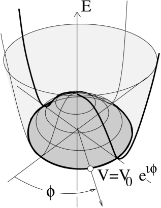
Figure 18: “Mexican Hat Potential” which determines minimum of Free energy, and self-consistently determines the width of the Kondo resonance. The Free energy displays this form provided the constraint $\partial F/\partial\lambda=\langle n_{f}\rangle-Q=0$ is imposed.

  Plotted as a function of $V$, this is the classic “Mexican Hat” potential, with a minimum where $\partial E/\partial V=0$ at $\Delta=\pi\rho|V|^{2}=T_{K}$. (Fig. 18)

• According to (146), the enhancement of the density of states at the Fermi energy is

  $$\rho^{*}(0) = \rho+\frac{\Delta}{\pi(\Delta^{2}+\lambda^{2})}$$ (159)

  $$= \rho+\frac{\sin(\pi q)}{\pi T_{K}}$$ (160)

  per spin channel. When the temperature is changed or a magnetic field introduced, one can neglect changes in $\Delta$ and $\lambda$, since the Free energy is stationary. This implies that in the large $N$ limit, the susceptibility and linear specific heat are those of a non-interacting resonance of width $\Delta$. The change in linear specific heat $\Delta C_{V}=\Delta\gamma T$ and the change in the paramagnetic susceptibility $\Delta\chi$ are given by

  $$\Delta\gamma = \left[\frac{N\pi^{2}k_{B}^{2}}{3}\right]\rho_{i}(0)=\left[\frac{N\pi^{2}k_{B}^{2}}{3}\right]\frac{\sin(\pi q)}{\pi T_{K}}$$ (161)

  $$\Delta\chi = \left[N\frac{j(j+1)(g\mu_{B})^{2}}{3}\right]\rho_{i}(0)=\left[N\frac{j(j+1)(g\mu_{B})^{2}}{3}\right]\frac{\sin(\pi q)}{\pi T_{K}}$$ (162)

  Notice how it is the Kondo temperature that determines the size of these two quantities. The dimensionless “Wilson” ratio of these two quantities is

  $$W=\left[\frac{(\pi k_{B})^{2}}{(g\mu_{B})^{2}j(j+1)}\right]\frac{\Delta\chi}{\Delta\gamma}=1$$

  At finite $N$, fluctuations in the mean-field theory can no longer be ignored. These fluctuations induce interactions amongst the quasiparticles, and the Wilson ratio becomes

  $$W=\frac{1}{1-\frac{1}{N}}.$$

  The dimensionless Wilson ratio of a large variety of heavy electron materials lies remarkably close to this value.

3.4 Gauge invariance and the composite nature of the $f-$electron

We now discuss the nature of the $f-$electron. In particular, we shall discuss how

• the $f-$electron is actually a composite object, formed from the binding of high-energy conduction electrons to the local moment.

• although the broken symmetry associated with the large $N$ mean-field theory does not persist to finite $N$, the phase stiffness associated with the mean-field theory continues to finite $N$. This phase stiffness is responsible for the charge of the composite $f$ electron.

3.4.1 Composite nature of the heavy $f-$electron

Let us begin by discussing the composite structure of the $f-$electron. In real materials, the Kondo effect we have described involves spins formed from localized f- or d-electrons. Though it is tempting to associate the composite $f-$electron in the Kondo effect with the the $f-$electron locked inside the local moment, we should also bear in mind that the Kondo effect could have occurred equally well with a nuclear spin! Nuclear spins do couple antiferromagnetically with a conduction electron, but the coupling is far too small for an observable nuclear Kondo effect. Nevertheless, we could conduct a thought experiment where a nuclear spin is coupled to conduction electrons via a strong antiferromagnetic coupling. In this case, a resonant bound-state would also form from the nuclear spin. The composite bound-state formed in the Kondo effect clearly does not depend on the origin of the spin partaking in the Kondo effect.

There are some useful analogies between the formation of the composite $f-$electron in the Kondo problem and the formation of Cooper pairs in superconductivity, which we shall try to draw upon. One of the best examples of a composite bound-state is the Cooper pair. Inside a superconductor, pairs of electrons behave as composite bosonic particles. One of the signatures of pair formation, is the fact that Cooper pairs of electron operators behave as a single composite at low energies,

$$\psi_{\uparrow}(x)\psi_{\downarrow}(x^{\prime})\equiv F(x-x^{\prime})$$

The Cooper pair operator is a boson, and it behaves as a c-number because the Cooper pairs condense. The Cooper pair wavefunction is extremely extended in space, extending out to distances of order $\xi\sim v_{F}/T_{c}$. A similar phenomenon takes place in the Kondo effect, but here the bound-state is a fermion and it does not condense For the Kondo effect the fermionic composite $(\vec{\sigma}\cdot\vec{S}(x))_{\alpha\beta}\psi_{\beta}(x)$ behaves as a single charged electron operator. The analogy between superconductivity and the Kondo effect involves the temporal correlation between spin-flips of the conduction sea and spin-flips of the local moment, so that at low energies

$$[\vec{\sigma}_{\alpha\beta}\cdot\vec{S}(t)]\psi_{\beta}(t^{\prime})\sim\Delta(t-t^{\prime})f_{\alpha}(t^{\prime}).$$

The function $\Delta(t-t^{\prime})$ is the analog of the Cooper pair wavefunction, and it extends out to times $\tau_{K}\sim{\mathchar 22\relax\mkern-9.0muh}/T_{K}$.

To see this in a more detailed fashion, consider how the interaction term behaves. In the path integral we factorize the interaction as follows

$$H_{I}=\frac{J}{N}\psi{{}^{{\dagger}}}_{\beta}\Gamma_{\alpha\beta}\psi_{\alpha}\longrightarrow\bar{V}\left(\psi{{}^{{\dagger}}}_{\beta}f_{\beta}\right)+\left(f{{}^{{\dagger}}}_{\beta}\psi_{\beta}\right)V+N\frac{\bar{V}V}{J}$$

By comparing these two terms, we see that the composite operator $\Gamma_{\alpha\beta}(j)\psi_{\alpha}(j)$ behaves as a single fermi field:

$$\frac{1}{N}\Gamma_{\alpha\beta}(t)\psi_{\alpha}(t)\longrightarrow\left(\frac{\bar{V}}{J}\right)f_{\beta}(t)$$ Evidently, a localized conduction electron is bound to a spin-flip of the local moment at the same site, creating a new independent fermionic excitation. The correlated action of adding a conduction electron with a simultaneous spin flip of the local moment at the same site creates a composite $f-$electron.
It is worth noting that this fermionic object only hybridizes with conduction electrons at a single point: it is thus local in space.

Let us now try to decompose the composite fermion in terms of the electrons that contribute to the bound-state amplitude. We start by writing the local moment in the fermionic representation,

$$\frac{1}{N}\Gamma_{\alpha\beta}\psi_{\alpha}=-\frac{1}{N}f{{}^{{\dagger}}}_{\alpha}\psi_{\alpha}f_{\beta}\longrightarrow-\frac{1}{N}\langle f{{}^{{\dagger}}}_{\alpha}\psi_{\alpha}\rangle f_{\beta}$$

where we have replaced the bilinear product between the conduction and $f-$electron by its expectation value. We can evaluate this “bound-state amplitude” from the corresponding Green-function

$$-\frac{V_{0}}{J}=\frac{1}{N}\langle f{{}^{{\dagger}}}_{\beta}\psi_{\beta}\rangle = \int\frac{d\omega}{\pi}f(\omega){\rm Im}G_{\psi f}(\omega-i\delta)$$ (163)

$$= V_{o}\int f(\omega)\frac{d\omega}{\pi}{\rm Im}\left[\sum_{k}\frac{1}{\omega-\epsilon_{k}-i\delta}\frac{1}{\omega-i\Delta}\right]$$ (164)

where we have chosen the half-filled case $Q/N=1/2$, $\lambda=0$. In the large band-width limit, the main contribution to this integral is obtained by neglecting the principal part of the conduction electron propagator $1/(\omega-\epsilon_{k}-i\delta)\rightarrow i\pi\delta(\omega-\epsilon_{k})$, so that

$$\frac{1}{N}\langle f{{}^{{\dagger}}}_{\beta}\psi_{\beta}\rangle = \sum_{k}f(\epsilon_{k})\left(\frac{\epsilon_{k}}{\epsilon_{k}^{2}+\Delta^{2}}\right)$$ (165)

From this expression, we can see that the contribution of a given $k$ state in the Fermi sea to the bound-state amplitude is given by

$$\frac{1}{N}\langle f{{}^{{\dagger}}}_{\beta}c_{k\beta}\rangle=f(\epsilon_{k})\left(\frac{\epsilon_{k}}{\epsilon_{k}^{2}+\Delta^{2}}\right)$$

This function decays with the inverse of the energy, right out to the band-width. Indeed, if we break-down the contribution to the overall bound-state amplitude, we see that each decade of energy counts equally. Let us take $T=0$ and divide the band on a logarithmic scale into $n$ equal parts, where the ratio of the lower and upper energies is $s>1$, then

$$\frac{V_{o}}{J} = \rho V_{o}\int_{-D}^{0}d\epsilon\frac{-\epsilon}{\epsilon^{2}+\Delta^{2}}\sim\rho V_{o}\int_{\Delta}^{D}d\epsilon\frac{1}{\epsilon}$$ (166)

$$= \rho V_{o}\left\{\int_{D/s}^{D}+\int_{D/s^{2}}^{D/s}+\dots\int_{D/s^{n}}^{D/s^{n-1}}+\int_{\Delta}^{{D/s^{n}}}\right\}\frac{d\epsilon}{\epsilon}$$ (167)

$$= \rho V_{0}\left\{\ln s+\ln s+\dots\ln s+\ln\frac{Ds^{-n}}{\Delta}\right\}$$ (168)

This demonstrates that the composite bound-state involves electrons spread out over decades of energy out to the band-width. If we complete the integral, we find that

$$\frac{V_{o}}{J}=\rho V_{o}\ln\frac{D}{\Delta}\Rightarrow\Delta=De^{-\frac{1}{J\rho}}=T_{K}$$

as expected from the minimization of the energy. Another way of presenting this discussion, is to write the composite bound-state in the time-domain, as

$$\frac{1}{N}\Gamma_{\alpha\beta}(t^{\prime})\psi_{\alpha}(t)\longrightarrow\Delta(t-t^{\prime})f_{\alpha}(t^{\prime})$$ (169)

where now

$$\Delta(t-t^{\prime})=\frac{1}{N}\langle f_{\beta}{{}^{{\dagger}}}(t)\psi_{\beta}(t^{\prime})\rangle$$

This is the direct analog of Cooper pair bound-state wavefunction, except that the relevant variable is time, rather than space. If one evaluates the function $\Delta(t)$ at a finite $t$, we find that

$$\Delta(t-t^{\prime})=\sum_{k}f(\epsilon_{k})\left(\frac{\epsilon_{k}}{\epsilon_{k}^{2}+\Delta^{2}}\right)e^{-i\epsilon_{k}(t-t^{\prime})}$$

Heuristically, the finite time cuts off the energy integral over the Fermi surface at an energy of order ${\mathchar 22\relax\mkern-9.0muh}/t$, so that

$$\Delta(t)\sim\left\{\begin{array}[]{lr}\rho V_{o}\ln\left(\frac{Dt}{{\mathchar 22\relax\mkern-9.0muh}}\right)&(t<<{\mathchar 22\relax\mkern-9.0muh}/T_{K})\cr\rho V_{o}\ln\left(\frac{D}{T_{K}}\right)&(t>>{\mathchar 22\relax\mkern-9.0muh}/T_{K})\end{array}\right.$$

emphasizing the fact that the Kondo effect involves a correlation between the spin-flips of the conduction sea and the local moment over decades of time scales from the the inverse band-width up to the Kondo time ${\mathchar 22\relax\mkern-9.0muh}/T_{K}$.

From these discussions, we see that the Kondo effect is

• entirely localized in space.

• extremely non-local in time and energy.

This picture of the Kondo effect as a temporal, rather than a spatial bound-state is vital if we are to understand the extension of the Kondo effect from the single impurity to the lattice.

3.4.2 Gauge invariance and the charge of the $f-$electron

One of the interesting points to emerge from the mean-field theory is that the energy of mean-field theory does not depend on the phase of the bound-state amplitude $V=|V|e^{i\theta}$. This is analogous to the gauge invariance in superconductivity, which derives from the conservation of the total electronic charge. Here, gauge invariance arises because there are no charge fluctuations at the site of the local moment, a fact encoded by the conservation of the total f-charge $Q$. Let us look at the full Lagrangian for the $f-$electron and interaction term

$${\cal L}_{I} = f_{\sigma}{{}^{{\dagger}}}(i\partial_{t}-\lambda)f_{\sigma}-H_{I}$$ (170)

$$H_{I} = \bar{V}\left(\psi{{}^{{\dagger}}}_{\alpha}f_{\alpha}\right)+\left(f{{}^{{\dagger}}}_{\alpha}\psi_{\alpha}\right)V+N\frac{\bar{V}V}{J}$$ (171)

This is invariant under the “Read-Newns”read transformation

$$f \rightarrow fe^{i\phi},$$ (172)

$$V \rightarrow Ve^{i\phi},\qquad\qquad(\theta\rightarrow\theta+\phi),$$ (173)

$$\lambda \rightarrow \lambda+\frac{\partial\phi}{\partial t}.$$ (174)

where the last relation arises from a consideration of the gauge invariance of the dynamic part $f{{}^{{\dagger}}}(i\partial_{t}-\lambda)f$ of the Lagrangian. Now if $V(t)=|V(t)|e^{i\theta(t)}$, where $V(t)$ is real, Read and Newns observed that by making the gauge choice $\phi(t)=-\theta(t)$, the resulting $V=|V|e^{i(\theta+\phi)}=|V|$ is real. In this way, once the Kondo effect takes place the phase of $V=|V|e^{i\theta}$ is dynamically absorbed into the constraint field $\lambda$ : effectively $\lambda\equiv\partial_{t}\phi$ represents the phase precession rate of the hybridization field. The absorption of the phase of an order parameter into a dynamical gauge field is called the “Anderson Higgs ” mechanism.andersonhiggs By this mechanism, once the Kondo effect takes place, $V$ behaves as a real, and hence neutral object under gauge transformations, this in turn implies that the composite $f-$electron has to transform under real electromagnetic gauge transformations, in other words the Anderson Higgs effect in the Kondo problem endows the composite $f-$electron with charge.

Table 1: Parallels between Superconductivity and the Kondo effect .

	Superconductivity	Kondo effect
Bound State	$\psi_{\uparrow}(x)\psi_{\downarrow}(x^{\prime})=F(x-x^{\prime})$	$\bigl{(}{\vec{\sigma}}_{\alpha\beta}\cdot{\vec{S}}(t^{\prime})\bigr{)}\psi_{\beta}(t)=\Delta(t-t^{\prime})f_{\alpha}(t^{\prime})$
	Bosonic	Fermionic
Characteristic energy	$T_{c}=\omega_{D}e^{-1/g\rho}$	$T_{K}=D\sqrt{J\rho}e^{-1/J\rho}$
Energy range contributing	$E\in[T_{c},\omega_{D}]$	$E\in[T_{K},D]$
to bound state
Extended in	space	time
	$\xi\sim v_{F}/T_{c}$	$\tau\sim{\mathchar 22\relax\mkern-9.0muh}/T_{K}$
Conserved Quantity	Total electron charge	Charge of local moment
Long Range Order	LRO $d>2$	Powerlaw in time
	Powerlaw in space $d\leq 2$
Phase stiffness	$\rho_{s}$	$\rho_{\phi}$
Consequences of	Meissner effect	Formation of charged
Phase stiffness		heavy electron
(Anderson- Higgs)		$2\frac{\Delta V_{F}}{(2\pi)^{3}}=n_{e}+n_{spins}$
Quantity related	$\frac{1}{\lambda_{L}^{2}}\propto\rho_{s}$	$\frac{1}{U^{*}}=\rho_{\phi}$
to phase stiffness

There is a paradox here, for in the Kondo effect, there can actually be no true broken symmetry, since we are dealing with a system where the number of local degrees of freedom is finite. Nevertheless, the phase $\phi$ does develop a stiffness- a stiffness against variation in time, and the order parameter consequently develops infinite range correlations in time. There is a direct analogy between the spatial phase stiffness of a superconductor and the temporal phase stiffness in the Kondo effect. In superconductivity, the energy depends on spatial derivatives of the phase

$$E\propto\frac{\rho_{s}}{2}(\nabla\phi-{2e}{}\vec{A})^{2}\Rightarrow\frac{1}{\lambda_{L}}^{2}\propto\rho_{s}$$

( where we have set ${\mathchar 22\relax\mkern-9.0muh}=1$.) Gauge invariance links this stiffness to the mass of the photon field, which generates the Meissner effect; the inverse squared penetration depth is directly proportional to the phase stiffness. In an analogous fashion, in the Kondo effect, the energy depends on temporal derivatives of the phase and the phase stiffness is

$$E\propto\frac{\rho_{\phi}}{2}(\partial_{t}\phi)^{2}$$

For a Kondo lattice, there is one independent Kondo phase for each spin site, and the independent conservation of $Q$ at each site guarantees that there is no spatial phase stiffness associated with $\phi$. The temporal phase stiffness leads to a slow logarithmic growth in the phase -phase correlation functions, which in turn leads to power-law temporal correlations in the order parameter $V(\tau)$:

$$\langle\delta\phi(\tau)\delta\phi(\tau^{\prime})\rangle\sim\frac{1}{N}\ln(\tau-\tau^{\prime}),\qquad\qquad\langle\bar{V}(\tau)V(\tau^{\prime})\rangle\sim e^{-\langle\delta\phi(\tau)\delta\phi(\tau^{\prime})\rangle}\sim(\tau-\tau^{\prime})^{-\frac{1}{N}}.$$

In this respect, the Kondo ground-state resembles a two dimensional superconductor, or a one dimensional metal: it is critical but has no true long-range order. As in the superconductor, the development of phase stiffness involves real physics. When we make a gauge transformation of the electromagnetic field,

$$e\Phi(x,t) \rightarrow e\Phi(x,t)+\partial_{t}\alpha(x,t),$$ (175)

$$e\vec{A}(x,t) \rightarrow e\vec{A}(x,t)+\nabla\alpha,$$ (176)

$$\psi(x) \rightarrow \psi(x)e^{-i\alpha(x,t)}$$ (177)

Because of the Anderson - Higgs effect, the hybridization is real and the only way to keep $L_{I}$ invariant under the above transformation, is by gauge transforming the $f-$electron and the constraint field

$$f_{\sigma}(j) \rightarrow f_{\sigma}(j)e^{-i\alpha(x_{j},t)}$$ (178)

$$\lambda \rightarrow \lambda+\partial_{t}\alpha$$ (179)

( Notice how $\lambda$ transforms in exactly the same way as the potential $e\Phi$.)

The non-trivial transformation of the $f-$electron under electromagnetic gauge transformations confirm that it has acquired a charge. Rigidity of the Kondo phase is thus intimately related to the formation of a composite charged fermion. The gauge invariant form for the energy dependence of the Kondo effect on the Kondo phase $\phi$ must then be

$$E\propto\frac{\rho_{\phi}}{2}(\partial_{t}\phi-{e}{}\Phi)^{2}$$

From the coefficient of $\Phi^{2}$, we see that the Kondo cloud has an intrinsic capacitance $C=e^{2}\rho_{\phi}$ ($E\sim C\Phi^{2}/2$). But since the energy can also be written $(en_{f})^{2}/2C\sim U^{*}n_{f}^{2}/2$ we see that the stiffness of the Kondo phase can also be associated with an interaction between the $f-$electrons of strength $U^{*}$, where

$$\frac{1}{U^{*}}=C/e^{2}={\rho_{\phi}}$$

3.5 Mean-field theory of the Kondo Lattice

3.5.1 Diagonalization of the Hamiltonian

We can now make the bold jump from the single impurity problem, to the lattice. Most of the methods described in the last subsection generalize very naturally from the impurity to the lattice: the main difficulty is to understand the underlying physics. The mean-field Hamiltonian for the latticeauerbach ; coleman87 takes the form

$$H_{MFT}=\sum_{\vec{k}\sigma}\epsilon_{\vec{k}}c{{}^{{\dagger}}}_{\vec{k}\sigma}c_{\vec{k}\sigma}+\sum_{j,\alpha}\left(f{{}^{{\dagger}}}_{j\alpha}\psi_{j\alpha}V_{o}+\bar{V}_{o}\psi{{}^{{\dagger}}}_{j\beta}f_{j\beta}+\lambda_{o}f{{}^{{\dagger}}}_{j\alpha}f_{j\alpha}\right)+{\cal N}N\left(\frac{\bar{V}_{o}V_{o}}{J}-\lambda_{o}q\right),$$

where $\cal N$ is the number of sites in the lattice. Notice, before we begin, that the composite f-state at each site of the lattice is entirely local, in that hybridization occurs at one site only. Were the composite f-state to be in any way non-local, we would expect that the hybridization of one f-state would involve conduction electrons at different sites. We begin by rewriting the mean field Hamiltonian in momentum space, as follows

$$H_{MFT}=\sum_{\vec{k}\sigma}\left(c{{}^{{\dagger}}}_{\vec{k}\sigma},f{{}^{{\dagger}}}_{\vec{k}\sigma}\right)\pmatrix{\epsilon_{\vec{k}}&\bar{V}_{o}\cr V_{o}&\lambda_{o}}\pmatrix{c_{\vec{k}\sigma}\cr f_{\vec{k}\sigma}}+{\cal N}N\left(\frac{\bar{V}_{o}V_{o}}{J}-\lambda_{o}q\right)$$

where

$$f{{}^{{\dagger}}}_{\vec{k}\sigma}=\frac{1}{\sqrt{\cal N}}\sum_{j}f{{}^{{\dagger}}}_{j\sigma}e^{i\vec{k}\cdot\vec{R}_{j}}$$

is the Fourier transform of the $f-$electron field. The absence of $k-$ dependence in the hybridization is evident that each composite $f-$electron is spatially local. This Hamiltonian can be diagonalized in the form

$$H_{MFT}=\sum_{\vec{k}\sigma}\left(a{{}^{{\dagger}}}_{\vec{k}\sigma},b{{}^{{\dagger}}}_{\vec{k}\sigma}\right)\pmatrix{E_{\vec{k}+}&0\cr 0&E_{\vec{k}-}}\pmatrix{a_{\vec{k}\sigma}\cr b_{\vec{k}\sigma}}+Nn\left(\frac{\bar{V}_{o}V_{o}}{J}-\lambda_{o}q\right)$$

where $a{{}^{{\dagger}}}_{\vec{k}\sigma}$ and $b{{}^{{\dagger}}}_{\vec{k}\sigma}$ are linear combinations of $c{{}^{{\dagger}}}_{\vec{k}\sigma}$ and $f{{}^{{\dagger}}}_{\vec{k}\sigma}$, playing the role of “quasiparticle operators” of the theory and the momentum state eigenvalues $E_{\vec{k\pm}}$ of this Hamiltonian are determined by the condition

$${\rm Det}\left[E_{\vec{k\pm}}\underline{1}-\pmatrix{\epsilon_{\vec{k}}&\bar{V}_{o}\cr V_{o}&\lambda_{o}}\right]=0,$$

which gives

$$E_{\vec{k}\pm}=\frac{\epsilon_{\vec{k}}+\lambda_{o}}{2}\pm\left[\left(\frac{\epsilon_{\vec{k}}-\lambda_{o}}{2}\right)^{2}+|V_{o}|^{2}\right]^{\frac{1}{2}}$$ (180)

are the energies of the upper and lower bands. The dispersion described by these energies is shown in Fig. 19 .

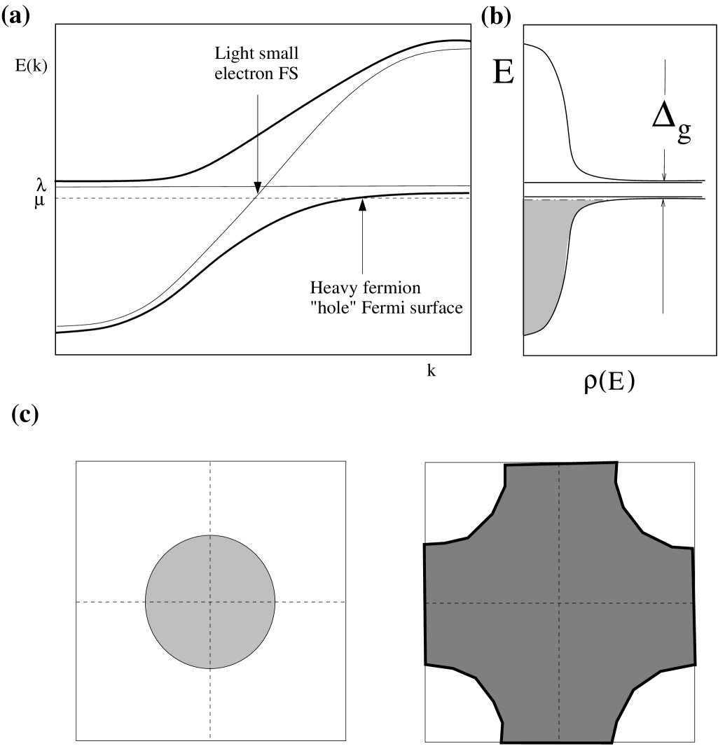
Figure 19: (a) Dispersion produced by the injection of a composite fermion into the conduction sea. (b) Renormalized density of states, showing “hybridization gap” ($\Delta_{g}$). (c) Transformation of the Fermi surface from a light electron Fermi surface into a heavy “hole”-like Fermi surface.

A number of points can be made about this dispersion:

• We see that the Kondo effect injects new fermionic states into the original conduction band. Hybridization between the heavy electron states and the conduction electrons builds an upper and lower Fermi band separated by a “hybridization gap” of width $\Delta_{g}=E_{g}(+)-E_{g}(-)$, such that energies in the range

  $$E_{g}(-)< E <\lambda_{o}+E_{g}(+)$$ (181)

  $$E_{g}(\pm) = \lambda_{o}\pm\frac{V_{0}^{2}}{D_{\mp}}$$ (182)

  are forbidden. Here $\pm D_{\pm}$ are the top and bottom of the conduction band. In the special case where $\lambda_{o}=0$, corresponding to half filling, a Kondo insulator is formed.

• The effective mass of the Fermi surface has the opposite sign to the original conduction sea from which it is built, so naively, the Hall constant should change sign when coherence develops.

• The Fermi surface volume expands in response to the presence of the new heavy electron bands. The new Fermi surface volume now counts the total number of particles. To see this note that

  $$N_{tot}=\langle\sum_{k\lambda\sigma}n_{k\lambda\sigma}\rangle=\langle n_{f}+n_{c}\rangle$$

  where $n_{k\lambda\sigma}=a{{}^{{\dagger}}}_{k\lambda\sigma}a_{k\lambda\sigma}$ is the number operator for the quasiparticles and $n_{c}$ is the total number of conduction electrons. This means

  $$N_{tot}=N\frac{V_{FS}}{(2\pi)^{3}}=Q+n_{c}.$$

  This expansion of the Fermi surface is a direct manifestation of the creation of new states by the Kondo effect. It is perhaps worth stressing that these new states would form, even if the local moments were nuclear in origin. In other words, it is only the rotational degrees of freedom of the local moments that are needed to form heavy electron bound-states with the conduction electrons.

The Free energy of this system is then

$$\frac{F}{N}=-T\sum_{\vec{k},\pm}\ln\biggl{[}1+e^{-\beta E_{\vec{k}\pm}}\biggr{]}+{\cal N}\left(\frac{\bar{V}V}{J}-\lambda q\right)$$

Let us discuss the ground-state energy, $E_{o}$ -the $T\rightarrow 0$ limit of this expression. We can write this in the form

$$\frac{E_{o}}{{\cal N}N}=\int_{-\infty}^{0}dE\rho^{*}(E)E+\left(\frac{\bar{V}V}{J}-\lambda q\right)$$

where we have introduced the density of heavy electron states $\rho^{*}(E)=\sum_{\vec{k},\pm}\delta(E-E^{(\pm)}_{\vec{k}})$. Now the relationship between the energy of the heavy electrons ($E$) and the energy of the conduction electrons ($\epsilon$) is given by

$$E=\epsilon+\frac{\bar{V}V}{E-\lambda}$$

so that the density of heavy electron states related to the conduction electron density of states $\rho$ by

$$\rho^{*}(E)=\rho\frac{d\epsilon}{dE}=\rho\left(1+\frac{\bar{V}V}{(E-\lambda)^{2}}\right)$$ (183)

The originally flat conduction electron density of states is now replaced by a “hybridization gap”, flanked by two sharp peaks of width approximately $\pi\rho V^{2}\sim T_{K}$. With this information, we can carry out the integral over the energies, to obtain

$$\frac{E_{o}}{{\cal N}N} = \frac{D^{2}\rho}{2}+\int_{-D}^{0}dE\rho{\bar{V}V}\frac{E}{(E-\lambda)^{2}}+\left(\frac{\bar{V}V}{J}-\lambda q\right)$$ (184)

$$= \frac{D^{2}\rho}{2}-\frac{\Delta}{\pi}\ln\left(\frac{D}{\lambda e}\right)+\left(\frac{\bar{V}V}{J}-\lambda q\right)$$ (185)

$$= \frac{D^{2}\rho}{2}-\frac{\Delta}{\pi}\ln\left(\frac{T_{K}}{\lambda e}\right)-\lambda q$$ (186)

where we have assumed that the upper band is empty, and the lower band is partially filled, and set $T_{K}=De^{-\frac{1}{J\rho}}$ as before. If we impose the constraint

$$\frac{\partial F}{\partial\lambda}=\langle n_{f}\rangle-Q=0$$ (187)

we obtain

$$\frac{\Delta}{\pi\lambda}-q=0$$

so that the ground-state energy can be written

$$\frac{E_{o}}{Nn_{s}}=\frac{\Delta}{\pi}\ln\left(\frac{\Delta e}{\pi qT_{K}}\right).$$ (188)

Let us pause for a moment to consider this energy functional qualitatively. The Free energy surface has the form of the “Mexican Hat” at low temperatures. The minimum of this functional will then determine a family of saddle point values $V=V_{o}e^{i\theta}$, where $\theta$ can have any value. If we differentiate the ground-state energy with respect to $V^{2}$, we obtain

$$0=\frac{1}{\pi}\ln\left(\frac{\Delta e^{2}}{\pi qT_{K}}\right)$$ (189)

or

$$\Delta=\frac{\pi q}{e^{2}}T_{K}$$ (190)

confirming that $\Delta\sim T_{K}$.

3.5.2 Composite Nature of the heavy quasiparticle in the Kondo lattice.

We now turn to discuss the nature of the heavy quasiparticles in the Kondo lattice. Clearly, at an operational level, the composite $f-$electrons are formed in the same way as in the impurity model, but at each site, i.e

$$\frac{1}{N}\Gamma_{\alpha\beta}(j,t)\psi_{j\alpha}(t)\longrightarrow\left(\frac{\bar{V}}{J}\right)f_{j\beta}(t)$$

This composite object admixes with conduction electrons at a single site- site j. The bound-state amplitude in this expression can be written

$$-\frac{\bar{V}_{o}}{J}=\frac{1}{N}\langle f{{}^{{\dagger}}}_{\beta}\psi_{\beta}\rangle$$ (191)

To evaluate the contributions to this sum, it is useful to notice that the condition $\partial E/\partial V=0$ can be written

$$\frac{1}{N}\frac{\partial E}{\partial V_{o}} = 0=\frac{\bar{V}_{o}}{J}+\frac{1}{N}\langle f{{}^{{\dagger}}}_{\beta}\psi_{\beta}\rangle$$ (192)

$$= \frac{\bar{V}_{o}}{J}+V_{o}\int_{-D}^{0}dE\rho\frac{E}{(E-\lambda)^{2}}$$ (193)

where we have used (184) to evaluate the derivative. From this we see that we can write

$$\frac{\bar{V}_{o}}{J} = -\bar{V}_{o}\int_{-D}^{0}dE\rho\left(\frac{1}{E-\lambda}+\frac{\lambda}{(E-\lambda)^{2}}\right)$$ (194)

$$= -V_{o}\rho\ln\left[\frac{\lambda e}{D}\right]$$ (195)

It is clear that as in the impurity, the composite $f-$electrons in the Kondo lattice are formed from high energy electron states all the way out to the bandwidth. In a similar fashion to the impurity, each decade of energy between $T_{K}$ and $D$ contributes equally to the overall bound-state amplitude. The above expression only differs from the corresponding impurity expression (163) at low energies, showing that low energy electrons play a comparatively unimportant role in forming the composite heavy electron. It is this feature that permits a dense array of composite fermions to co-exist throughout the crystal lattice.

These composite $f-$electrons admix with the conduction electrons to produce a heavy electron band with a density of states given by (183),

$$\rho^{*}(E)=\rho\frac{d\epsilon}{dE}=\rho\left(1+\frac{V_{0}^{2}}{(E-\lambda)^{2}}\right)$$

which, setting $E=0$ and using (187) and (190), becomes

$$\rho^{*}(0)=\rho+\frac{q}{\lambda}=\rho+\frac{qe^{2}}{T_{K}}$$

at the Fermi energy. The mass enhancement of the heavy electrons is then

$$\frac{m^{*}}{m}=1+\frac{qe^{2}}{\rho T_{K}}\sim\frac{qD}{T_{K}}$$

This large factor in the effective mass enhancement can be as much as $1000$ in the most severely renormalized heavy electron systems.

3.5.3 Consequences of mass renormalization

The effective mass enhancement of heavy electrons can be directly observed in a wide range of experimental quantities including

• The large renormalization of the linear specific heat coefficient $\gamma^{*}\sim\frac{m^{*}}{m}\gamma$ and Pauli susceptibility $\chi^{*}\sim\frac{m^{*}}{m}\chi$.

• The quadratic temperature (“ A” ) coefficient of the resistivity. At low temperatures the resistivity of a Fermi liquid has a quadratic temperature dependence, $\rho\sim\rho_{o}+AT^{2}$, where $A\sim\left(\frac{1}{T_{F}}\right)^{2}\sim\left(\frac{m^{*}}{m}\right)^{2}\sim\gamma^{2}$ is related to the density of three-particle excitations. The approximate constancy of the ratio $A/\gamma^{2}$ in heavy fermion systems is known as the “Kadowaki-Woods” relation.kadowaki

• The renormalization of the effective mass as measured by dHvA measurements of heavy electron Fermi surfaces.onuki ; lonzarich1 ; lonzarich2

• The appearance of a heavy quasiparticle Drude feature in the frequency dependent optical conductivity $\sigma(\omega)$. (See discussion below).

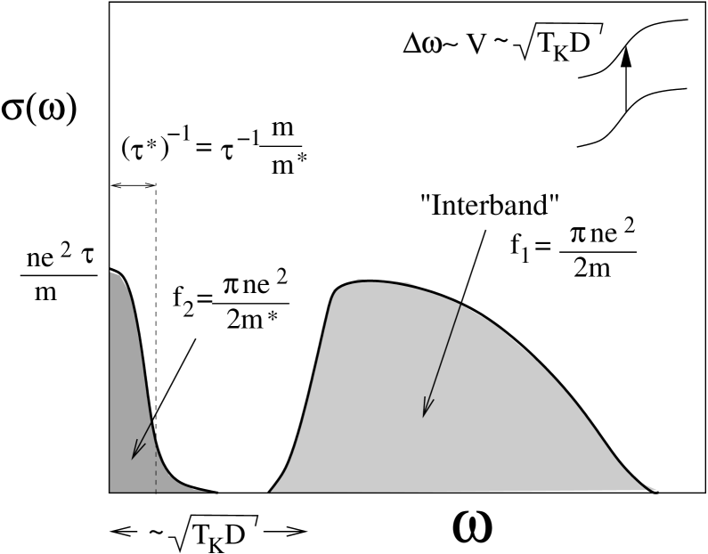
Figure 20: Separation of the optical sum rule in a heavy fermion system into a high energy “inter-band” component of weight $f_{2}\sim ne^{2}/m$ and a low energy Drude peak of weight $f_{1}\sim ne^{2}/m^{*}$.

The optical conductivity of heavy fermion metals deserves special discussion. According to the f-sum rule, the total integrated optical conductivity is determined by the plasma frequency

$$\int_{0}^{\infty}\frac{d\omega}{\pi}\sigma(\omega)=f_{1}=\frac{\pi}{2}\left(\frac{ne^{2}}{m}\right)$$

where $n$ is the density of electrons. In the absence of local moments, this is the total spectral weight inside the Drude peak of the optical conductivity.

What happens to this spectral weight when the heavy electron fluid forms? Whilst we expect this sum rule to be preserved, we also expect a new “quasiparticle” Drude peak to form in which

$$\int{d\omega}\sigma(\omega)=f_{2}\frac{\pi}{2}\frac{ne^{2}}{m^{*}}=f_{1}\frac{m}{m^{*}}$$

In other words, we expect the total spectral weight to divide up into a tiny “heavy fermion” Drude peak, of total weight $f_{2}$, where

$$\sigma(\omega)=\frac{ne^{2}}{m^{*}}\frac{1}{(\tau^{*})^{-1}-i\omega}$$

is split off by an energy of order $V\sim\sqrt{T_{K}D}$ from an “inter-band” component associated with excitations between the lower and upper Kondo bands.millis ; anders This second term carries the bulk $\sim f_{1}$ of the spectral weight. (Fig. 20 ).

Simple calculations, based on the Kubo formula confirm this basic expectation,millis ; anders showing that the relationship between the original relaxation rate of the conduction sea and the heavy electron relaxation rate $\tau^{*}$ is

$$(\tau^{*})^{-1}=\frac{m}{m^{*}}(\tau)^{-1}.$$ (196)

Notice that this means that the residual resistivity

$$\rho_{o}=\frac{m^{*}}{ne^{2}\tau^{*}}=\frac{m}{ne^{2}\tau}$$

is unaffected by the effects of mass renormalization. This can be understood by observing that the heavy electron Fermi velocity is also renormalized by the effective mass, $v_{F}^{*}=\frac{m}{m^{*}}$, so that the mean-free path of the heavy electron quasiparticles is unaffected by the Kondo effect.

$$l^{*}=v_{F}^{*}\tau^{*}=v_{F}\tau$$

This is yet one more reminder that the Kondo effect is local in space, yet non-local in time.

These basic features- the formation of a narrow Drude peak, and the presence of a hybridization gap, have been seen in optical measurements on heavy electron systemsschlesinger ; gruner88 ; gruner97

3.6 Summary

In this lecture we have presented Doniach’s argument that the enhancement of the Kondo temperature over and above the characteristic RKKY magnetic interaction energy between spins leads to the formation of a heavy electron ground-state. This enhancement is thought to be generated by the large spin degeneracies of rare earth, or actinide ions. A simple mean-field theory of the Kondo model and Kondo lattice, which ignores the RKKY interactions, provides a unified picture of heavy electrons and the Kondo effect. The essential physics involves composite quasiparticle formation between high energy conduction band electrons and local moments. This basic physical effect is local in space, but non-local in time. Certain analogies can be struck between Cooper pair formation, and the formation of the heavy electron bound-state, in particular, the charge on the $f-$electron can be seen as a direct consequence of the temporal phase stiffness of the Kondo bound-state. This bound-state hybridizes with conduction electrons- producing a single isolated resonance in a Kondo impurity, and an entire renormalized Fermi surface in the Kondo lattice.

3.7 Exercises

1. 1. Directly confirm the Read-Newns gauge transformation (172).

   2. Directly calculate the “phase stiffness” $\rho_{\phi}=-\frac{d^{2}F}{d\lambda^{2}}$ of the large $N$ Kondo model and show that at $T=0$.

      $$\rho_{\phi}=\frac{N}{\pi}\left(\frac{\sin(\pi q)}{T_{K}}\right).$$

2. 1. Introduce a simple relaxation time into the conduction electron propagator, writing

      $$G(\vec{k},i\omega_{n})^{-1}=i\omega_{n}+i{\rm sgn}(\omega_{n})/2\tau+\frac{V^{2}}{i\omega_{n}-\lambda}$$ (197)

      Show that the poles of this Greens function occur at

      $$\omega=E_{k}\pm\frac{i}{2\tau^{*}}$$

      where

      $$\tau^{*}=\frac{m^{*}}{m}\tau$$

      is the renormalized elastic scattering time.

   2. The Kubo formula for the optical conductivity of an isotropic one-band system is

      $$\sigma(\nu)=-\frac{Ne^{2}}{3}\sum_{k}v_{k}^{2}\frac{\Pi(\nu)}{i\nu}$$

      where we have used the $N$ fold spin degeneracy, and $\Pi(\nu)$ is the analytic extension of

      $$\Pi(i\nu_{n})=T\sum_{m}G(\vec{k},i\omega_{m})\left[G(\vec{k},i\omega_{m}+i\nu_{n})-G(\vec{k},i\omega_{m})\right]$$

      where in our case, $G(\vec{k},i\omega_{n})$ is the conduction electron propagator. Using (197), and approximating the momentum sum by an integral over energy, show that the low frequency conductivity of the large $N$ Kondo lattice is given by

      $$\sigma(\nu)=\frac{ne^{2}}{m^{*}}\frac{1}{(\tau^{*})^{-1}-i\nu}.$$

4 Quantum Criticality in Heavy Electron Systems

4.1 Introduction

This section provides a brief introduction to the unsolved problem of quantum criticality in heavy fermion materials. Many of the ideas summarized here are the result of collaborations, and much of the material in this section is published in review form. questions ; susy ; susy2 Heavy electron materials lie on the verge of magnetic instability. In the discussion of the last section, we ignored magnetism and focussed on the dense Kondo effect. What happens when they are pushed to the very edge of magnetic instability? Such a question was first posed in the context of itinerant magnetic order in a pioneering work by John Hertz, almost thirty years ago. Hertz concluded that a metallic system at the edge of magnetic instability would develop a new kind of critical behavior- quantum critical behavior.

A quantum critical point (QCP) is a zero-temperature instability between two phases of matter where quantum fluctuations develop long range correlations in both space and timesachdevbook . At a finite temperature critical point, the critical long-wavelength fluctuations of the order parameter do not involve quantum mechanics. This is because thermal fluctuations destroy the coherence of quantum fluctuations on time-scales longer than

$$\tau\sim\frac{{\mathchar 22\relax\mkern-9.0muh}}{k_{B}T},$$ (198)

The great revolution in our understanding of critical phenomena which occured in the 1970s involved many tools borrowed from relativistic field theory, but the physics was entirely classical.

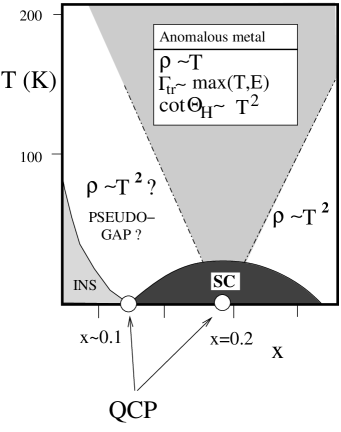
Figure 21: Schematic phase diagram for cuprate superconductors showing location of possible quantum critical points. One of these QCP may be responsible for the anomalous normal state which develops above the pseudogap scale.

Experimental developments of the past decade have brought a new awareness of the importance of quantum critical points in condensed matter physics. These special points exert a profound influence on the finite temperature properties of a material. Materials close to quantum criticality develop a new excitation structure, they display novel thermodynamic, transport and magnetic behavior. They also have marked a predeliction towards the development of new kinds of order, such as anisotropic superconductivity. A dramatic example is provided by the cuprate superconductors. By doping with holes, these materials pass through one or more quantum phase transitions: from an insulator to a metal with a spin gap at low doping, and at higher doping a second QPT appears to occur when the spin gap closes loram (Fig. 21) The singular interactions induced by quantum criticality are thought to the driving force for both the high temperature superconductivity and the anomalous metallic state above the spin gap temperature $T^{*}$.castellani

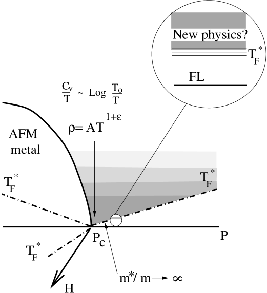
Figure 22: Illustration of quantum critical physics in heavy fermion metals. As criticality is approached from either side of the transition, the temperature scale $T_{F}^{*}$ on which Fermi liquid behavior breaks down goes to zero. A key challenge is to characterize the new class of universal excitations which develops above $T_{F}^{*}$.

Heavy Fermion materials offer a unique opportunity to study quantum criticality under controlled conditions. By the application of pressure, doping and most recently, magnetic field, these materials can be tuned through a quantum critical point from a metallic antiferromagnet into a paramagnet (Fig. 22). Unlike the cuprate metals, here the paramagnetic phase is a well characterized Fermi liquid,landau ; early ; early2 with heavy Landau quasiparticles, or “heavy electrons”. A central property of these quasiparticles, is the existence of a finite overlap “$Z$” between a single quasiparticle state, denoted by $|\hbox{qp}^{-}\rangle$ and the state formed by adding a single electron to the ground-state, denoted by $|e^{-}\rangle=c{{}^{{\dagger}}}_{{\bf k}\sigma}|0\rangle$. This quantity is closely related to the ratio $m/m^{*}$ of the electron to quasiparticle mass,

$$Z=|\langle e^{-}|\hbox{qp}^{-}\rangle|^{2}\sim\frac{m}{m^{*}}.$$ (199)

A wide body of evidence suggests that $m^{*}/m$ diverges at a heavy fermion QCP, indicating that

$$Z\rightarrow 0\qquad\qquad(\hbox{$P\rightarrow P_{c}$}).$$

The state which forms above the QCP is referred to as a “non-Fermi” or “singular Fermi liquid”. continentino ; varma2001 ; questions ; questions2 ; stewart2001 By what mechanism does this break-down in the Landau quasiparticle occur?

Table. 1. Selected Heavy Fermion compounds with quantum critical points. Compound $x_{c}$/$P_{c}$/$H_{c}$ $\frac{C_{v}}{T}\rightarrow\infty$? $\rho\sim T^{a}$ Ref. $YbRh_{2}Si_{2-x}Ge_{x}$ $x_{c}=0.1$ $Log\left(\frac{T_{o}}{T}\right)$ ^∗ $T$ steglich $CeCu_{6-x}Au_{x}$ $x_{c}=0.1$ $Log\left(\frac{T_{o}}{T}\right)$ $T+c$ hilbert1 ; hilbert2 ; schroeder $CeCu_{6-x}Ag_{x}$ $x_{c}=0.09$ $Log\left(\frac{T_{o}}{T}\right)$ $T^{1.1}$ heuser $CeNi_{2}Ge_{2}$ $P_{c}=0$ $Log\left(\frac{T_{o}}{T}\right)$^∗ $T^{1.2}$ grosche ; gegenwart ; julian ; braithwaite ; newgegen $U_{2}Pt_{2}In$ $P_{c}=0$ $Log\left(\frac{T_{o}}{T}\right)$ $T$ devisser $U_{2}Pd_{2}In$ $P_{c}<0$ ? $T+c$ devisser $CePd_{2}Si_{2}$ $P_{c}>0$ ? $T^{1.2}$ grosche $CeCoIn_{5}$ $P_{c}\sim 1.6GPa$ ? $T$ sarrao $CeIn_{3}$ $P_{c}>0$ ? $T^{1.5}$ grosche ; mathur $U_{3}Ni_{3}Sn_{4}$ $P_{c}>0$ no ? devisser2 $CeCu_{2}Si_{2}$ $P_{c}=0$ no $T^{1.5}$ cecu2si2 $CeRu_{2}Si_{2}$ $H^{\parallel}_{c}=7.7T$ $Log\left(\frac{T_{o}}{T}\right)$ aoki2 $UPt_{3}$ $H^{\perp}_{c}=20T$ $Log\left(\frac{T_{o}}{T}\right)$ $T^{1.2}$ stewartupt3 $Sr_{3}Ru_{2}O_{7}$ $H^{\parallel}_{c}=7.7T$ $Log\left(\frac{T_{o}}{T}\right)$ $T^{1.1}$ mackenzie

^∗ New datanewgegen ; gegenwart show a stronger divergence at lower temperatures.

4.2 Properties of the Heavy Fermion Quantum Critical Point

There is a growing list of heavy fermion systems that have been tuned to an antiferromagnetic QCP by the application of pressure or by doping (Table 1.). These materials display many common properties

• Fermi liquid behavior in the paramagnet, as indicated by the emergence of a quadratic temperature dependence in the resistivity in the approach to the QPT $\rho=\rho_{o}+AT^{2}$ devisser2 ; flouquet at ever lower temperatures.

• Divergent A coefficient in resistivity at the QCP. In a typical Fermi liquid the $A$ coefficient in the resistivity is proportional to $\left(\frac{1}{1/T_{F}^{*}}\right)^{2}\sim\left(\frac{m^{*}}{m}\right)^{2}$, where $T_{F}^{*}$ is the Fermi temperature. Support for the divergence of the effective mass is provided by the observation that the quadratic coefficient $A$ of the resistivity grows, and apparantly diverges at the quantum critical pointdevisser .

• Divergent specific heat at the QCP, with an asymptotic logarithmic temperature dependence,

  $$\gamma(T)=\frac{C_{v}(T)}{RT}=\frac{Q}{T_{o}}\log\left[\frac{T_{o}}{T}\right]+\gamma_{n},$$ (200)

  where $R$ is the gas constant, and experimentally ${Q}\approx 0.4$, suggesting that the Fermi temperature vanishes and the quasiparticle effective masses diverge

  $$T_{F}^{*}\rightarrow 0,\qquad\frac{m^{*}}{m}\rightarrow\infty$$ (201)

  at the QCP. The above expression has been written in a form where the characteristic energy $T_{o}$ enters both inside the logarithm and in the prefactor. There are a number of materials where this one-parameter form holds, with $\gamma_{n}=0$, suggesting a new kind of universality where no normal component to the Fermi surface survives at the QCP. sereni

• Quasi-linear resistivity

  $$\rho\propto T^{1+\epsilon},$$ (202)

  at the QCP with $\epsilon$ in the range $0-0.6$. In critical $YbRh_{2}Si_{2-x}Ge_{x}$, $\rho\propto T$ over three decadessteglich00 .

• Non-Curie spin susceptibilities

  $$\chi^{-1}(T)=\chi_{0}^{-1}+cT^{a}$$ (203)

  with $a<1$ observed in critical $CeCu_{6-x}Au_{x}$ (x=0.1), $YbRh_{2}Si_{2-x}Ge_{x}$ (x=0.1) and $CeNi_{2}Ge_{2}$.

• $E/T$ and $H/T$ Scaling. In critical $CeCu_{6-x}Au_{x}$ and $YbRh_{2}Si_{2-x}Ge_{x}$ the differential magnetic susceptibility $dM/dH$ exhibits $H/T$ scaling,

  $$(dM/dH)^{-1}=\chi_{0}^{-1}+cT^{a}g[H/T],$$ (204)

  where $a\approx 0.75$. Neutron measurementsschroeder show $E/T$ scalingvarma1989 ; aronson in the dynamical spin susceptiblity of critical $CeCu_{6-x}Au_{x}$, throughout the Brillouin zone, parameterized in the form

  $$\chi^{-1}({\bf q},\omega)=T^{a}f(E/T)+\chi_{0}^{-1}({\bf q})$$ (205)

  $F[x]\propto(1-ix)^{a}$. Scaling behavior with a single anomalous exponent in the momentum-independent component of the dynamical spin susceptibility suggests an emergence of local magnetic moments which are critically correlated in time at the quantum critical pointschroeder .

4.3 Universality

Usually, the physics of a metal above its Fermi temperature depends on the detailed chemistry and band-structure of the material: it is non-universal. However, if the renormalized Fermi temperature $T^{*}_{F}(P)$ can be tuned to become arbitrarily small compared with the characteristic scales of the material as one approaches a QCP, we expect that the “high energy” physics above the Fermi temperature $T^{*}_{F}$ is itself, universal.

Quantum critical behavior implies a divergence of the long distance and long-time correlations in the material. Finite temperatures introduce the cutoff timescale

$$\tau_{T}=\frac{{\mathchar 22\relax\mkern-9.0muh}}{k_{B}T}$$ (206)

beyond which coherent quantum processes are dephased by thermal fluctuations. Renormalization group principleshertz imply that the quantum critical physics has an upper-critical dimension $d_{u}$. For $d<d_{u}$, $\tau_{T}$ becomes the correlation time $\tau$ of the systemzinnjustin , so frequency dependent correlation functions and response functions take the form

$$F(\omega,T)=\frac{1}{\omega^{\alpha}}f(\omega\tau_{T})=\frac{1}{\omega^{\alpha}}f({\mathchar 22\relax\mkern-9.0muh}\omega/k_{B}T).$$ (207)

leading to $E/T$ scalingsachdev . By contrast, for $d>d_{u}$ the correlation time is sensitive to the details of the short-distance interactions between the critical modes, and in general $\tau^{-1}\propto T^{1+b}$, ($b>0$). Thus $E/T$ scaling with a non-trivial exponent strongly suggests that the underlying physics of the heavy fermion quantum critical point is governed by universal physics with $d_{u}>3$.

4.4 Failure of the Spin Density Wave picture

The standard model of the heavy fermion QCP assumes the non-Fermi liquid behavior derives from Bragg diffraction of the electrons off a quantum-critical spin density wave (QSDW)hertz ; paladium ; moriya ; millis . The virtual emission of these soft fluctuations,

$$e^{-}\rightleftharpoons e^{-}+\hbox{spin fluctuation}$$ (208)

generates a retarded interaction

$$V_{eff}({\bf q},\omega)=g^{2}\overbrace{\left[\frac{\chi_{0}}{({\bf q}-{\bf Q})^{2}+\xi^{-2}-\frac{i\omega}{\Gamma_{\bf Q}}}\right]}^{{\chi({\bf q},\omega)}}$$ (209)

between the electrons, where $\chi({\bf q},\omega)$ is the dynamical spin susceptibility of the collective modes. The damping term $-i\omega/\Gamma_{{\bf Q}}$ of the magnetic fluctuations is derived from the linear density of particle-hole states in the Fermi sea. $\xi^{-1}$ and $\tau^{-1}=\Gamma_{{\bf Q}}\xi^{-2}$ are the inverse spin correlation length and correlation times respectively. In real space,

$$V_{eff}(r,\omega=0)\propto\frac{e^{-r/\xi}}{r}e^{i{\bf Q}\cdot{\bf r}}$$ (210)

is a “modulated ” Yukawa potential whose range $\xi\sim(P-P_{c})^{-\frac{1}{2}}\rightarrow\infty$ at the QCP. Unlike a ferromagnetic QCP, the modulated potential only affects electron quasiparticles along “hot lines” on the Fermi surface, that are separated by the wave-vector $\bf Q$ and satisfy $\epsilon_{\bf k}=\epsilon_{{\bf k}+{\bf Q}}$. At a finite temperature, electrons within a momentum range $\sim\sqrt{T}$ are affected by this critical scattering (Fig. 23.). This limits the ability of this singular potential to generate non Fermi liquid behavior.

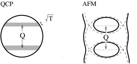
Figure 23: Quantum spin density wave scenario, where the Fermi surface “folds” along lines separated by the magnetic $Q$ vector, pinching off into two separate Fermi surface sheets.

There are then two major difficulties with the (three dimensional) QSDW scenario for the heavy fermion QCP:

1. No breakdown of the Fermi liquid Away from the hot lines, the Fermi surface and Landau quasiparticles remain intact at the QCP. Thus the specific heat and typical quasiparticle mass do not diverge but exhibit a weaker singularity, $C_{V}/T=\gamma_{o}-A\sqrt{T}$ in the QSDW picturemillis .

2. No $E/T$ scaling The quantum critical behavior predicted by this model has been extensively studiedhertz ; millis . In the interaction $V_{eff}({\bf q},\omega)$ the momentum dependence enters with twice the power of the frequency, so

   $$\tau\sim\xi^{z},\qquad(z=2).$$

   In the renormalization group (RG) treatmenthertz time counts as $z$ space dimensions so the effective dimensionality is $D_{eff}=d+z=d+2$. The upper critical dimension is set by $D_{eff}=4$, or $d_{u}=2$millis , so 3D quantum spin fluctuations will not lead to $E/T$ scaling. In three dimensions, QSDW theory predicts that the scale entering into the energy dependent response functions should scale as $T^{3/2}$, with a non-universal prefactorsachdevbook .

4.5 Towards a new understanding.

In this last lecture, I would like to give you a sense of the seriousness of the failure of the spin density wave scenario and share with you some of the new ideas that are circulating. Some have argued that it may be possible to explain the of $E/T$ scaling and the logarithmically divergent specific heatrosch by supposing that the spin fluctuations form a quasi-two-dimensional spin fluidmathur ; rosch , lying at the critical dimension. Inelastic neutron scattering experiments on $CeCu_{6-x}Au_{x}$, (x=0.1) support a kind of reduced dimensionality in which the critical scattering is concentrated along linear, rather than at point-like regions in reciprocal spaceschroeder ; rosch . More recent datafak may support quasi-2D spin fluctuations at intermediate scales in $CeGe_{2}Ni_{2}$.

The assumption that the spin fluid is two dimensional is hard to reconcile with the fact that the developing order is fully three dimensional, and with the fact that these systems exhibit very little dimensional anisotropy. Even if we accept these problems, there other difficulties. First- quasi-two dimensionality can furnish $E/T$ scaling, but it does not drop the theory below its critical dimension, and hence has no way of accounting for the anomalous exponents in the $E/T$ scaling.

Finally, there is another more serious difficulty. It has recently become possible to examine the approach to the heavy electron quantum critical point through the use of field tuningstewart ; stewartupt3 ; gegen2002 . The material $YbRh_{2}Si_{2-x}Ge_{x}$ with $x=0.1$ lies precisely at a quantum critical point. By applying a small magnetic field, this system is driven back into the Fermi liquid. As the field is reduced and the system is tuned back towards the quantum critical point, the $A$ coefficient of the resistivity is observed to diverge as

$$A\propto\frac{1}{B}$$

Such behavior can be obtained in a two dimensional spin fluid model in which the inverse squared correlation length is assumed to be proportional to $B$, $\xi^{-2}\propto B$. The same model predicts a weak dependence of the linear specific heat on magnetic field

$$\gamma_{th}\propto Log(1/B)$$

so that the ratio

$$\frac{A_{th}}{\gamma_{th}^{2}}\sim\frac{1}{BLog(1/B)}.$$

The same experiments also show that the linear specific heat diverges much more rapidly with $B$, as $\gamma\propto\frac{1}{\sqrt{B}}$, so that the Kadowaki Woods ratio

$$A/\gamma^{2}=constant.$$ (211)

It is difficult to understate the importance of this new result. The constancy of the Kadowaki Woods ratio over more than a decade in $\gamma$ indicates that the momentum dependence of the scattering amplitudes in the Fermi liquid are not radically affected by the magnetic field, as they would be if the chief mechanism for the mass renormalization were derived from the exchange of soft magnetic fluctuations in a 2D spin fluid. These new results can only be understood if, in the approach to the quantum critical point, the Fermi liquid scattering amplitudes remain local, depending only on the size of the renormalized Fermi temperature $T_{F}^{*}$coleman87 .

(212)

$$\raisebox{-28.90755pt}[0.0pt][0.0pt]{\psfig{width=86.72377pt}}=F_{k,k^{\prime},k-q}=T_{F}^{*}{\cal F}(\frac{E_{\vec{k}}}{T_{F}^{*}},\frac{E_{\vec{k}^{\prime}}}{T_{F}^{*}},\frac{E_{\vec{k}-\vec{q}}}{T_{F}^{*}};\vec{k},\vec{k}^{\prime},\vec{q})$$ (213)

In the previous chapter, I argued that the effective Fermi temperature of the Kondo lattice measures the “phase stiffness” associated with the amplitude to form of a composite heavy electron, so that

$$\rho_{\phi}\sim{T_{F}^{*}}.$$

The constancy of the Kadowaki Woods ratio, the lock-step divergence of both $A$ and $\gamma^{2}$, and the appearance of local features in the spin correlations at the quantum critical point are all in keeping with the idea that the Kondo bound-state phase stiffness is going to zero on the paramagnetic side of the heavy electron quantum critical point, just as the spin-wave stiffness $\rho_{M}$ goes to zero on the magnetic side of the same point. In other words

$$\left.\begin{array}[]{rcl}\rho_{\phi}&\longrightarrow&0,\cr\rho_{M}&\longrightarrow&0\end{array}\right\}\hbox{\text@underline{quantum bicriticality?} }$$ (217)

In other words, the Kondo composite bound-state appears to die at exactly the same time magnetic order develops. This strongly suggests to me, that perhaps the heavy electron quantum critical point might be better understood as a quantum bicritical point, where two order parameters go to zero at a point.

Traditionally, theories of phase transition are built apon an underlying mean-field theory. The spin density wave scenario is a consequence of examining fluctuations about the Stoner and Slater view of itinerant magnetism. If this approach fails, then perhaps it is a sign that we should search for a new kind of mean-field theory to describe the quantum phase transition between antiferromagnetism and the heavy electron fluid. There are two kinds of suggestion that have been considered recently :

• Local quantum criticality. The apparent momentum independence of the localized critical correlations at the quantum critical pointschroeder has led to the suggestion that the the correct mean-field theory, is one that is local, yet fully dynamical.xsach ; sengupta ; siandsmith Such “dynamical mean-field theories”,krauth are thought to asymptotically exact in infinite dimensions. In this philosophy, the local physics remains strongly interacting even in infinite dimensions, but the local character of the interactions is supposed to be stable against finite dimensionality. This idea forms the basis of a recent theory by Si et al.

• Traditional RG approach on a new Lagrangian. Rather than abandon the traditional RG approach first suggested by Hertz,hertz we should continue to embrace the notion that a Wilsonian approach, where interactions become weak in high enough dimensions does work for quantum critical points. This approach argues that what is needed, is a new description of magnetism, and the way it couples to the Fermi sea. One idea here, is that at the quantum critical point, the heavy electron breaks up into its spin and charge components.questions2

We now discuss these ideas in more depth.

4.6 Local Quantum Criticality

The momentum-independent scaling term in the inverse dynamic susceptibility (7) suggests that the critical behavior associated with the heavy fermion QCP contains some kind of local critical excitationschroeder . One possibility, is that this critical excitation is the spin itself, which would then presumably develop a slow power-law decayxsach ; sengupta ; siandsmith

$$\langle S(\tau)S(\tau^{\prime})\rangle=\frac{1}{(\tau-\tau^{\prime})^{2-\epsilon}},$$ (218)

where $\epsilon\neq 0$ signals non- Fermi liquid behavior.

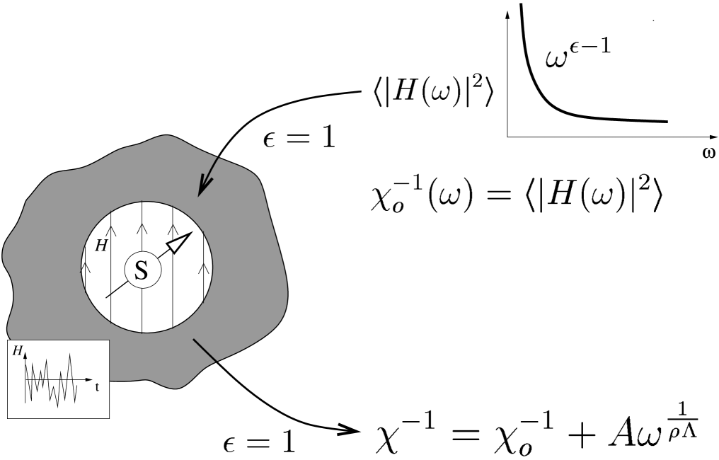
Figure 24: In the local quantum critical theory, each spin behaves as a local moment in a fluctuating Weiss field. In the theory of Si et al [102], a self-consistent solution can be obtained for $\epsilon=1$ in which the local susceptibility develops a self-energy with a non-universal exponent. $M(\omega)\propto\omega^{\frac{1}{\rho\Lambda}}$.

Sisi et al. have extensively developed this idea, proposing that the local spin susceptibility $\chi_{loc}=\sum_{\vec{q}}\chi(\vec{q},\omega)|_{\omega=0}$ diverges at a heavy fermion QCP. From (205),

$$\chi_{loc}(T)\sim\int d^{d}q\frac{1}{({\bf q}-{\bf Q})^{2}+T^{\alpha}}\sim T^{(d-2)\alpha/2}$$ (219)

so a divergent local spin susceptibilty requires a spin fluid with $d\leq 2$. Si et al are thus motivated to propose that the non-trivial physics of the heavy fermion QCP is driven by the formation of a two-dimensional spin fluid. Si et al consider an impurity spin within an effective medium in which the local Weiss field $H$ has a critical power-spectrum (Fig. 24.)

$$\langle|H(\omega)|^{2}\rangle\equiv\chi_{0}^{-1}(\omega)=\omega^{\gamma}$$ (220)

where $\epsilon$ is self-consistently evaluated using a dynamical mean-field theory, where $q-$ dependence of self-energies is dropped. In principle, the method solves the dynamical spin susceptibility of the impurity $\chi^{-1}(\omega)=\chi_{o}^{-1}(\omega)+M(\omega)$. This, in turn furnishes a “spin self-energy” $M(\omega)$ used to determine the spin susceptibility of the medium $\chi^{-1}(\vec{q},\omega)=J(\vec{q})+M(\omega)$.

Si et al find that a self-consistent solution is obtained for $\epsilon=1$, if the spin-self energy contains a separate power-law dependence $M(\omega)\sim\omega^{\alpha}$ with an exponent $\alpha=1/\rho\Lambda$ which is determined by the density of states $\rho$ and band-width $\Lambda$ of the bond-strengths in the two-dimensional spin fluid. Although self-consistency requires a new power-law in the spin susceptibility, independent solutions of the impurity model have not yet shown that this feature is indeed generated by a critical Weiss field. This theory nevertheless raises many interesting questions:

1. Is the requirement of a two dimensional spin fluid consistent with the ultimate emergence of three dimensional magnetic order. For example- does the the cubic (and hence manifestly three dimensional) quantum critical material, $CeIn_{3}$ display a divergent specific heat?

2. If the spin-fluids are quasi-two dimensional, do we expect an ultimate cross-over to a three-dimensional QSDW scenario?

3. If $\alpha$ is non-universal, why are the critical exponents in $CeCu_{6-x}Au_{x}$ and $YbRh_{2}Si_{2-x}Ge_{x}$ so similar?

4. What stabilizes the local quantum criticality against intersite couplings?

4.7 Ideas of spin charge separation and supersymmetry.

An alternative possibility, is that the heavy fermion QCP is a truly three-dimensional phenomenon. In this case a different approach is needed- we need to search for a new class of critical Lagrangian with $d_{u}>3$susy . On general grounds, the existence of a Fermi liquid in the paramagnetic phase suggests that the new class of critical Lagrangians must find expression in terms of the quasiparticle fields $\psi$ in the Fermi liquid- but how do we couple these degrees of freedom to the magnetism, and how do we account for the simultaneous loss of the resonant bound-state stiffness at the same time that magnetism develops? The simplest possibility is to write

$$L=L_{F}[\psi]+L_{F-M}[\psi,M]+L_{M}[M].$$ (221)

where $L_{F}$ describes the heavy Fermi liquid, far from the magnetic instability, $L_{M}$ describes the magnetic excitations that emerge above the energy scale $T_{F}^{*}(P)$.

$L_{F-M}$ describes the way that the quasiparticles couple to and decay into critical magnetic modes; it also determines the type of transformation which takes place in the Fermi surface which occurs at the QCP. This last point follows because away from the QCP, magnetic fluctuations can be ignored in the ground-state, so that $L_{M}\rightarrow 0$. In the paramagnetic phase, $\langle M\rangle=0$ so $L_{FM}\rightarrow 0$, but in the antiferromagnetic phase $\langle M\rangle\neq 0$, i.e.

$${{L}}_{\hbox{eff}}=\left\{\begin{array}[]{cl}{L}_{F}^{*}[\psi]&\ \hbox{paramagnet}\cr\cr{L}_{F}^{*}[\psi]+{L}_{FM}[\psi,\langle M\rangle]&\ \hbox{a.f.m.}\end{array}\right.$$

where the asterisk denotes the finite renormalizations derived from zero-point fluctuations in the magnetization.

If the staggered magnetization is the fundamental critical field, then we are forced to couple the magnetic modes directly to the spin density of the Fermi liquid

$$L_{F-M}^{(1)} = g\sum_{{\bf k},{\bf q}}\psi{{}^{{\dagger}}}_{\vec{k}-\vec{q}}\vec{\sigma}\psi_{\vec{k}}\cdot\vec{M}_{{\bf q}}.$$ (222)

But once the staggered magnetization condenses, this leads directly back to a static spin density wave (Fig 23).

An alternative possibility is suggested by the observation that the magnetism develops spinorial character in the heavy Fermi liquid. The Luttinger sum ruleluttinger governing the Fermi surface volume $V_{FS}$ “ counts” both the electron density $n_{e}$ and the number of local moments per unit cell $n_{{spins}}$martin82 ; oshikawa00 :

$$2\frac{{\cal V}_{FS}}{(2\pi)^{3}}=n_{e}+n_{spins}.$$ (223)

The appearance of the spin density in the Luttinger sum rule reflects the composite nature of the heavy quasiparticles, formed from bound-states between local moments and high energy electron states. Suppose the spinorial character of the magnetic degrees of freedom seen in the paramagnet also manifests itself in the decay modes of the heavy quasiparticles. This would imply that at the QCP, the staggered magnetization factorizes into a spinorial degree of freedom $\vec{M}(x)=z{{}^{{\dagger}}}(x)\vec{\sigma}z(x)$, where $z$ is a two-component spin $1/2$ Bose field. “Spinorial magnetism” affords a direct coupling between the magnetic spinor $z$ and the heavy electron quasi-particles via an inner product, over the spin indices

$$L_{F-M}^{(2)}=g\sum_{{\bf k},{\bf q}}[\chi_{\bf q}{{}^{{\dagger}}}\left(z{{}^{{\dagger}}}_{{\bf k}-{\bf q}\sigma}\psi_{{\bf k}\sigma}\right)+\hbox{H.c}],$$ (224)

where conservation of exchange statistics obliges us to introduce a spinless charge $e$ fermion $\chi$. This would imply that the composite heavy electron decays into a neutral “spinon”and a spinless charge e fermion $e^{-}_{\sigma}\rightleftharpoons s_{\sigma}+\chi^{-}$. The critical Lagrangian in this case would take the form

$$L=L_{F}[\psi]+L_{F-M}[\psi,\chi,z]+L_{M}[z,\psi].$$ (225)

We have to be cautious of course, because this is undoubtedly one of many alternative ways we might begin to construct a new class of critical Lagrangians. What we do see quite clearly however, is this line of reasoning leads us to into the notion that the break-up of the heavy fermion QCP involves spin-charge separation.

Hall constant measurements may provide a good way to discern between the spin density wave and composite quasiparticle alternatives. In the former, regions around the hot-line do not contribute to the Hall conductivity, and the change in the Hall constant is expected to evolve as the staggered magnetizationquestions2 . By contrast, the composite fermion scenario leads to a much more rapid evolution: provided that the density of spinless fermions is finite at the QCP the Hall constant will jump suddenly at the QCP questions .

$$\Delta R_{H}\propto\left\{\begin{array}[]{cr }M_{\bf Q},&\qquad\hbox{(vectorial )}\cr O(1)&(\hbox{spinorial})\end{array}\right.$$ (226)

The only available Hall measurement at a QCP to date shows a change in sign takes place in the close vicinity of the QCP in critical $CeCu_{6-x}Au_{x}$, it is not yet clear whether there is a discontinuity at the transitiononuki00 . This is clearly an area where more experimental input is highly desirable.

Let me end with a few speculations. If we are to construct a new critical theory for the heavy electron quantum critical point, then we will need some new theoretical ideas. A new critical theory will require as a first step, a new kind of mean-field description that permits us to understand why the magnetism and the Kondo effect die at a common critical point. At present, we do not know how to construct a mean-field theory that contains a heavy electron quantum critical point. One interesting idea here, may be the incorporation of supersymmetry. This is an idea that I have tried to develop, as yet with only partial success, with my graduate student John Hopkinson and collaborators, Catherine Pépin and Alexei Tsvelik.susy ; susy2 At a very naive level, magnetism involves the manifestation of spin as a bosonic excitation, whereas heavy electron behavior involves the manifestation of spin as a fermionic object. If the two phenomena share the same quantum critical point, then is it possible that the spin manifests both types of behavior at a quantum critical point- in otherwords, that it displays some kind of supersymmetry?

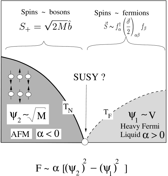
Figure 25: The heavy fermion QCP may involve a supersymmetric gauge symmetry. To understand the fact that the magnetization ($M$) disappears at precisely the same point in the phase diagram where the amplitude ($V$) for the formation of composite fermions goes to zero, we need a special symmetry between the two order parameters. Local moments behave as fermions in the paramagnetic phase, but as bosons in the antiferromagnet. Does a supersymmetry develop at the quantum critical point and is this responsible for the “Minkowskii” metric between the two order parameters that is required for them to vanish at the same point in the phase diagram?

It does prove possible to represent both spin and Hubbard operators in a way that involves a locally supersymmetric gauge theory, but a mean-field theory still eludes us at the current time. We do have an idea about the structure of this mean-field theory, which I shall briefly mention to you. In this putative mean-field theory, we require two order parameters- one for the formation of the composite heavy electron corresponding to the amplitude for composite fermion formation $\psi_{1}\sim V$ and one for the magnetism ($\psi_{2}\sim\langle z_{\sigma}\rangle\sim\sqrt{M}$). Suppose we can integrate out all of the fermions in the theory, so that we are left with an effective theory for $\psi_{1}$ and $\psi_{2}$, given by a Landau Ginzburg free energy $F[\psi_{1},\psi_{2}]$. Now here’s the remarkable thing- for the two order parameters to share a quantum critical point, then the expansion of the Free energy near the QCP must take the form

$$F\sim\alpha(|\psi_{2}|^{2}-|\psi_{1}|^{2})+\hbox{interactions}$$

When $\alpha>0$, we have the heavy electron phase with $\psi_{2}=0,\qquad\psi_{1}\neq 0$ but when $\alpha<0$, we have the magnetic phase, where $\psi_{2}\neq 0,\qquad\psi_{1}=0$. At $\alpha=0$, both order parameters vanish simultaneously. The two must go to zero at the same point in the phase diagram, so they can only come together in the quadratic combination $(|\psi_{1}|^{2}-|\psi_{2}|^{2})$. This suggests that the negative definite metric

$$(|\psi_{2}|^{2}-|\psi_{1}|^{2})$$

is a symmetry invariant of the quantum critical point. The appearance of a minus sign - a Minkowskii type metric- is required by the phenomenology, yet traditional invariant symmetry groups of a critical point involve a positive metric associated with a trace over order parameter combinations. The minus sign would occur if the residual symmetry between these two order parameters corresponded to symplectic group. One way for such minus signs might appear is via the supertrace- an invariant of a supergroup. This prompts the following conjecture, on which I will end: that the the above invariance is a residue of a supertrace in a supersymmetric Lagrangian for quantum criticality.

4.8 Summary

This section has discussed the origin of the mass divergence at the heavy fermion quantum critical point, emphasizing that a quantum spin density wave picture can not explain the observed properties. The proposal of fundamentally new kinds of quantum critical points has been reviewed. This is clearly an area with a huge potential for progress both on the experimental, and theoretical front.

4.9 Exercises

1. Consider the tree level scaling for the zero temperature Hertz-Millis Lagrangian at an antiferromagnetic quantum critical point

   $$S=S_{K}+S_{I}$$ (227)

   where

   $$S_{K} = \int^{|\omega|<\omega_{o},k<\Lambda}\frac{d\omega d^{d}k}{(2\pi)^{d+1}}\chi^{-1}(\kappa)M(\kappa)M(-\kappa)$$ (228)

   $$\chi^{-1}(\kappa) = \left[(\vec{k}-\vec{Q})^{2}+\frac{|\omega|^{2/z}}{\Gamma}\right]$$ (229)

   describes the propagation of an overdamped spin fluctuation with inverse susceptibility $\chi^{-1}(\vec{k},\omega)$ at quantum criticality, with a critical wavevector $\vec{Q}$. Here we have used the notation $\kappa\equiv(\vec{k},\omega)$ to denote the wavevector and frequency of a magnetization mode. The non-linear interaction term in the model takes the form

   $$S_{I}[U]=U\int\left(\prod_{j=1,4}\frac{d^{(d+1)}\kappa_{j}}{(2\pi)^{d+1}}\right)M(\kappa_{1})\dots M(\kappa_{4})\delta^{d+1}(\sum_{j}\kappa_{j})$$ (230)

   1. Derive the tree level scaling that keeps the Kinetic term $S_{K}$ invariant. First note that from the kinetic term, the scaling dimension of frequency is $[\omega]=[k]^{z}$. Show that if the wavevector and frequency cut-off are rescaled according to

      $$\tilde{\Lambda}=\frac{\Lambda}{b},\qquad\tilde{\omega_{0}}=\frac{\omega_{0}}{b^{z}}$$ (231)

      then one must rescale

      $$k=\tilde{k}b,\qquad\omega=\tilde{\omega}b^{z}$$ (232)

      to keep the form of the Kinetic term invariant. Show that under this scaling

      $$S_{K}\rightarrow b^{(z+d-2)}\int^{|\tilde{\omega}|<\omega_{o},\tilde{k}<\Lambda}\frac{d^{d+1}\tilde{\kappa}}{(2\pi)^{d+1}}\chi^{-1}(\tilde{\kappa})M(\kappa)M(-\kappa)$$

      so that with scaling

      $$M(\kappa)=\tilde{M}(\tilde{\kappa})b^{-(z+d-2)/2}$$

      the kinetic energy remains invariant.

   2. Using the tree level scaling derived above, show that the interaction term transforms as

      $$S_{I}(U)\rightarrow S_{I}(U^{*})$$

      where

      $$U^{*}=\frac{U}{b^{(z+d-4)}}$$

      showing that the interaction term scales to zero for $d+z>4$, proving that $d=4-z=2$ is the upper-critical dimension for the Hertz-Millis model.

References

- (1) See for example A. C. Hewson The Kondo Problem to Heavy Fermions (Cambridge: Cambridge University Press), also D. Cox and M. B. Maple “Electronic Pairing in Exotic Superconductors”, Physics Today 48, 2, 32, (1995).
- (2) J. K. Jain, Science 266, 1199 (1994). For more more details, “Perspectives in Quantum Hall Effects” edited by S. Das Sarma and A. Pinczuk (Wiley, New York , 1997); “Composite Fermions” edited by Olle Heinonen (World Scientific, New York, 1997)
- (3) Leo Kouwenhoven and Leonid Glazman- ‘The revival of the Kondo effect’ Physics World, 14, 1, 33-38, cond-mat/0104100 and references therein.
- (4) See for example, P. Coleman, “Condensed Matter, Strongly Correlated Electron Physics”, Physics World Issue 12, 29 (1995). and P. W. Anderson, “Condensed Matter Physics, the Continuous Revolution”, Physics World Issue 12, 37 (1995).
- (5) For an elementary introduction to cuprate superconductivity, see Gerald Burns, “High Temperature Superconductivity: an Introduction”, Boston- Academic Press (1992.)
- (6) P. W. Anderson, “Basic Notions of Condensed Matter Physics”,Benjamin Cummings (1984).
- (7) A. M. Clogston, B.T. Matthias,M. Peter, H. J. Williams, E. Corenzwit and R. C. Sherwood, Phys. Rev. 125, 541 (1962).
- (8) P. W. Anderson, Phys. Rev 124, 41, 1961.
- (9) J. Friedel, Nuovo Cimcento (Suppl.) 2, 287 (1958).
- (10) A. Blandin & J. Friedel, J. Phys. Radium , 19 , 573 , (1958).
- (11) J. Kondo in Solid State Physics 23, eds F. Seitz, D. Turnbull and H. Ehrenreich p (183), New York, Academic Press.
- (12) Greg Stewart Rev Mod Phys 56, 755, (1984).
- (13) D. Langreth, Phys. Rev. 150, 516, (1966).
- (14) J. R. Schrieffer and P. Wolff, Phys. Rev. 149, 491, 1966.
- (15) B. Coqblin and J. R. Schrieffer, Phys. Rev. 185, 847, 1969.
- (16) Anderson P. W. & G. Yuval, Phys. Rev. Lett. 45, 370, 1969; Anderson P. W. & G. Yuval, Phys. Rev. B 1, 1522, 1970; Anderson P. W. & G. Yuval, J. Phys. C 4, 607, 1971.
- (17) P. W. Anderson, Comm. S. St. Phys. 5, 72, 1973; Journal of Physics C 3, 2346, 1970.
- (18) K. G. Wilson, Rev. Mod. Phys 47, 773, 1976.
- (19) P. Nozières, Journal de Physique C 37, C1-271, 1976 ; P. Nozières and A. Blandin, Journal de Physique 41, 193, 1980.
- (20) M. Sarachik, E. Corenzwit and L. D. Longinotti, Phys Rev. 135, A1041 (1964).
- (21) A. M. Clogston, B. T. Mathias, M. Peter, H. J. Williams, E. Corenzwit and R. C. Sherwood, Phys. Rev. 125, 541 (1962).
- (22) Robert H. White and Theodore H. Geballe, Long Range Order in Solids, Academic Press, New York (1979), pp 278.
- (23) B. Triplett, Ph. D. Thesis, U. California, Berkeley (1970).
- (24) F. T. Hedgcock and C. Rizzuto, Phys. Rev 163 , 517 (1963).
- (25) S. M. Cronenwett, T. H. Oosterkamp, and L. P. Kouwenhoven, Science 281, 540 (1998).
- (26) W. G. van der Wiel et al., Science 289, 2105 (2000).
- (27) E. Bucher et al, Phys. Rev. B, 11, 440 (1975).
- (28) F. Steglich , J. Aarts. C. D. Bredl, W. Leike, D. E. Meshida, W. Franz & H. Schäfer, Phys. Rev. Lett. 43, 1892, 1976.
- (29) H. R. Ott, H. Rudgier, Z. Fisk and J. L. Smith, Phys. Rev. Lett 50, 1595, (1983).
- (30) M. A. Ruderman and C. Kittel, Phys. Rev. 78, 275, 1950; T. Kasuya, Prog. Theo. Phys. 16, 45, 1956; K. Yosida, Phys. Rev. 106, 896, 1957.
- (31) K. Andres , J. Graebner & H. R. Ott., Phys. Rev. Lett. 35, 1779, (1975).
- (32) S. Doniach, Valence Instabilities and Narrow Band Phenomena, edited by R. Parks, 34, (Plenum 1977); S. Doniach, Physica B91, 231 (1977).
- (33) The Kondo lattice Hamiltonian was first written down, with a Ferromagnetic exchange by T. Kasuya, Prog. Theo. Phys 16, 45 (1956). In this respect, it holds the distinction of being the oldest electronic model in condensed matter theory, probably the first to be written down in second quantized form.
- (34) Mekata M, S. Ito, N. Sato and T. Satoh, Journal of Magnetism and Magnetic Materials, 54, 433 (1986).
- (35) Y. Onuki and T. Komatsubara, Journal of Magnetism and Magnetic Materials, 63-64, 281 (1987).
- (36) R. M. Martin, Phys. Rev. Lett. 48, 362 (1982).
- (37) M. Oshikawa, Phys. Rev. Lett. 84, 3370 (2000).
- (38) To obtain heavy fermion behavior in transition metal systems one needs magnetic frustration. A good example of such behavior is provided by the pyrochlore transition metal heavy fermion system, , see C. Urano, M. Nohara, S. Kondo, F. Sakai, H. Takagi, T. Shiraki and T. Okubo, Phys. Rev. Lett. 85, 1052 (2000).
- (39) P. W. Anderson in “Valence Fluctuations in Solids”, North Holland (Amsterdam, 1981).
- (40) E. Witten, Nucl. Phys. B 145,110 (1978).
- (41) A. A. Abrikosov, Physics 2, 5, 1965.
- (42) H. Suhl, Phys. Rev. 138A, 515, 1965.
- (43) F. D, M. Haldane Phys. Rev. Lett. 40, 416 , 1978.
- (44) H. R. Krishnamurthy, J. Wilkins and K. G. Wilson, Phys. Rev. B 21 , 1003, 1980.
- (45) C. Lacroix and M. Cyrot, Phys. Rev. B 43, 12906, 1991.
- (46) N. Read, D.M. Newns and S. Doniach, Phys. Rev. B20, 384 (1984).
- (47) See for example, Dieter Forster, “Hydrodynamic fluctuations, broken symmetry and correlation functions” (Advanced Book Classics, Perseus Books, 1990).
- (48) A. Auerbach and K.Levin, Phys. Rev. Lett. 57, 877, 1986.
- (49) P. Coleman, Phys. Rev. Lett. 59, 1026 (1987).
- (50) K. Kadowaki and S. B. Woods, Solid State Comm. 58, 507 (1986).
- (51) P. H. P. Reinders, M. Springford et al, Phys. Rev. Letters 57, 1631, (1986).
- (52) L. Taillefer and G. G. Lonzarich, Phys. Rev. Lett. 60, 1570, (1988).
- (53) S. R. Julian, G. J. McMullan, C. Pfleiderer, F. Tautz and G. G. Lonzarich, J. Appl. Phys 76, 6137 (1994).
- (54) L. Degiorgi, F.Anders and G. Gruner, European Physical Journal B, 19, 167 (2001).
- (55) B. Bucher, Z. Schlessinger, D. Mandrus, Z. Fisk, J. Sarrao, J. F. DiTusa, C. Oglesby, G. Aeppli and E. Bucher, Phys. Rev B 53,R2948 (1995).
- (56) W. P. Beyerman, G. Gruner, Y. Dlicheouch and M. B. Maple, Phys. Rev. B 37, 10353 (1988).
- (57) S. Donovan, A. Schwartz and G. Gruner, Phys. Rev. Lett 79, 1401 (1997).
- (58) S. Sachdev, “Quantum Phase Transitions”, ( Cambridge University Press, 1999 ).
- (59) D. Obertelli, J. R. Cooper and J. L. Tallon, Phys. Rev. B46, 14928 (1992).
- (60) C. Castellani, C. Di Castro and M. Grilli, Z. Phys. B 103, 137 (1997);J. Tallon et al, Phys. Stat. Solidi (b) 215, 531 (1999).
- (61) L. D. Landau, Soviet Physics, JETP 3, 920 (1957), (Zh. Eksp. Teor. Fiz. 30, 1058 (1956)).
- (62) D. Pines and P. Nozières, “The Theory of Quantum Liquids” (Benjamin, New York, 1966), vol 1.
- (63) P. Nozières, “Theory of Interacting Fermi Systems”, (Benjamin, New York, 1964).
- (64) M. Continentino, “Quantum Scaling in Many-Body Systems”, Mucio A. Continentino, World Scientific Lecture Notes in Physics, vol. 67 (World Scientific, New York, 2001.)
- (65) C. M. Varma, Z. Nussinov and W. van Saarlos, “Singular Fermi Liquids”, submitted to Physics Reports, cond-mat/0103393.
- (66) G. Stewart, “Non-Fermi-liquid behavior in d- and f- band metals”, Rev. Mod. Phys. 73, 797-855, (2001).
- (67) P. Coleman, C. Pépin, Qimiao Si and Revaz Ramazashvili, J. Phys. Cond. Matt 13 273 (2001).
- (68) P. Coleman and C. Pépin, “What is the fate of the heavy electron at a quantum critical point?”, Physica B: Condensed Matter, 312-313, 383 (2002).
- (69) O. Trovarelli, C.Geibel, S. Mederle, C. Langhammer, F.M. Grosche, P. Gegenwart, M. Lang, G. Sparn and F. Steglich, Phys. Rev. Lett. 85 ,626 (2000).
- (70) H. v. Lohneysen et al. Phys. Rev Lett bf 72, 3262 (1994).
- (71) H. v. Lohneysen, J. Phys. Cond. Mat. bf 8, 9689-9706 (1996).
- (72) A. Schroeder et al., Nature 407, 351(2000).
- (73) K. Heuser et al., Phys. Rev. B57, R4198 (1998).
- (74) M. Grosche et al., J. Phys. Cond Matt 12, 533(2000).
- (75) P. Gegenwart, F. Kromer, M. Lang, G. Sparn, C. Geibel and F. Steglich, Phys. Rev. Lett 82, 1293 (1999).
- (76) S.R. Julian et al., J. Phys. Cond. Mat. 8, 9675 (1996).
- (77) D. Braithwaite, T. Fukuhara, A. Demeur, I. Sheikin, S. Kambe, J-P. Brison, K. Maez, T. Naka and J. Floquet, J. Phys. Cond. Matt 12, 1339 (2000).
- (78) O. Trovarelli et al, to be published (2001).
- (79) P. Estrela, A. de Visser, T. Naka, F.R. de Boer, L. C. J Pereira, cond-mat/0106292, proceedings of SCES 2001.
- (80) V. A. Sidorov, M. Nicklas, P. G. Pagliuso, J. L. Sarrao, Y. Bang, A. V. Balatsky and J. D. Thompson, cond-mat/0202251, (2002)
- (81) N. Mathur et al. Nature 394,39 (1998).
- (82) P. Estrela, A. de Visser, F.R. de Boer, T. Naka and L. Shlyk, Phys. Rev. B63, 212409 (2001).
- (83) P. Gegenwart et al. Phys. Rev. Lett. 81, 1501 (1998).
- (84) Y. Aoki et al, Journal of Magnetism and Magnetic Materials 177-181, 271 (1998).
- (85) J. S. Kim, D. Hall, K. Heuser and G. R. Stewart, Solid State Comm. 114, 413 (2000).
- (86) R. S. Perry et al., Phys. Rev. Lett. 86, 2661 (2001).
- (87) G. Knebel, D. Braithwaite, P. Canfield, G. Lapertot and J. Flouquet, to be published (2001).
- (88) J. G. Sereni, C. Geibel, M. G. -Berisso, P. Hellmann, O. Trovarelli and F. Steglich, Physica B 230-232,580-582 (1997).
- (89) scaling was first introduced as part of the Marginal Fermi Liquid phenomenology by C. M. Varma, P. B. Littlewood, S. Schmitt-Rink, E. Abrahams and A. E. Ruckenstein, Phys. Rev. Lett. 30, 1996 (1989).
- (90) scaling was first observed in the disordered non-Fermi liquid material , M.C. Aronson, R. Osborn, R.A. Robinson, J.W. Lynn, R. Chau, C.L. Seaman, and M.B. Maple, Phys. Rev. Lett. 75, 725 (1995).
- (91) J. A. Hertz, Phys. Rev. B 14, 1165 (1976).
- (92) J. Zinn-Justin, Quantum Field Theory and Critical Phenomena, chap 30 p. 710 ( Oxford University Press, 1993).
- (93) S. Sachdev and J. Ye, Phys. Rev. Lett. 69, 2411 (1992).
- (94) M. T. Beal-Monod, Physica 109 & 110B, 1837 (1982).
- (95) T. Moriya and J. Kawabata, J. Phys. Soc. Japan 34, 639 (1973); J. Phys. Soc. Japan 35,669 (1973).
- (96) A. J. Millis, Phys. Rev. B 48, 7183 (1993).
- (97) O. Stockert, H.v. Lohneysen, A. Rosch, N. Pyka, M. Loewenhaupt, Phys. Rev. Lett. 80, 5627 (1998).
- (98) B. Fak, J. Flouquet, G. Lapertot, T. Fukuhara, H. Kadowaki, J. Phys. Cond. Matt 12, 5423 (2000).
- (99) J. Custers et al., to be published (2002).
- (100) S. Sachdev and J. Ye, Phys. Rev. Lett. 70, 3339 (1993).
- (101) A. Sengupta, Phys. Rev. B 62, 4041, (2000).
- (102) J. L. Smith and Q. Si, Europhys. Lett 45, 224 (1999).
- (103) A. Georges, G. Kotliar, W. Krauth and M. Rozenberg, Rev. Mod. Phys. 68, 13 (1996).
- (104) Q. Si, S. Rabello, K. Ingersent and J. L. Smith, Nature 413, 6858, 804 (2001).
- (105) S. Doniach, Physica B 91, 231 (1977).
- (106) P. Coleman, C. Pépin, A. M. Tsvelik, Phys. Rev. B, 62, 3852-3868 (2000).
- (107) P. Coleman, C. Pépin, and J. Hopkinson, Phys. Rev. B, 63,140411(R), (2001).
- (108) J. M. Luttinger and J. C. Ward, Phys Rev. 118, 1417 (1960), J. M. Luttinger, Phys. Rev. 119, 1153 (1960).
- (109) T. Nakimi, H. Sato, J. Jrakawa, H. Sugawara, Y. Aoki, R. Settai and Y. Onuki, Physica B 281-282, 359 (2000).