Pseudogap Kondo Physics from Charge Fluctuations in a Quantum Dot

Abstract

We consider charge fluctuations in a quantum dot coupled to an interacting one-dimensional electron liquid. We find the behavior of this system to be similar to the multichannel pseudogap Kondo model. By tuning the coupling between the dot and the one-dimensional electron liquid, one can access the quantum critical point and the various fixed points which arise. The differential capacitance is computed and is shown to contain detailed information about the system.

Nanotechnology has been the source of a renewed interest in the Kondo effect.leo The incredible progress in miniaturizing solid state devices has made it possible to fabricate small metallic islands (i.e. quantum dots) by confining electrons in a two-dimensional electron gas. Quantum dots provide a highly controllable environment to study Kondo physics, and allow for many aspects of the Kondo effect to be probed. In this work, we suggest that a quantum dot coupled to an interacting one-dimensional electron liquid (i.e. a Luttinger liquid) could provide a controlled environment to observe pseudogap Kondo physics.

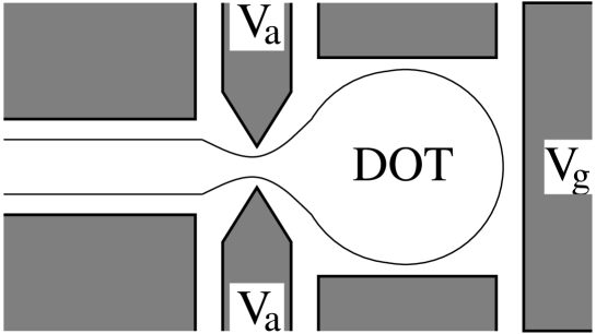
Figure 1: Setup: A quantum dot coupled to an interacting one-dimensional electron liquid. The number of electrons on the dot is controlled by the gate voltage $V_{g}$. A voltage applied to the auxiliary gates, $V_{a}$, controls the coupling between the dot and the one-dimensional electron liquid.

The pseudogap Kondo model was first considered in Ref. withoff, . In this model, a magnetic impurity is coupled to a sea of conduction electrons with a density of states vanishing at the Fermi energy with power-law behavior

$$H_{\rm int}=J~{}{\bf\tau}\cdot\frac{{\bf\sigma}_{s,s^{\prime}}}{2}\psi^{\dagger}_{s}(0)\psi^{\phantom{\dagger}}_{s}(0)\ \ \ {\rm with}\ \ \ \rho(E)=\rho_{0}|E|^{r}\,.$$

One of the most interesting features of this model is that, for antiferromagnetic coupling ($J>0$), there is an unstable intermediate coupling fixed point occurring when $J=J_{c}$. For $J<J_{c}$, the impurity spin is unscreened at low energies; for $J>J_{c}$ the impurity spin is screened. At $J=J_{c}$, the impurity spin exhibits quantum critical fluctuations. It is worth mentioning that this model has attracted attention recently due to its potential relevance to various correlated electron systems. In particular, this model has been argued to describe impurities in high-$T_{c}$ cuprate superconductors. zinc Moreover, the critical behavior occuring when $J=J_{c}$ may be relevant to the behavior seen in heavy fermion materials.si2 ; si1

The setup we consider is shown in Fig. 1. A large quantum dot is coupled to a reservoir, consisting of an interacting one-dimensional electron liquid. The dot is capacitively coupled to a gate; the gate voltage $V_{g}$ controls the number of electrons on the dot. The coupling between the dot and the reservoir is controlled by a voltage $V_{a}$ applied to the auxiliary gates. To model the dot, we assume the level spacing of the dot is much smaller than any energy scale in the problem; we approximate the spectrum of the dot by a single particle continuum. Moreover, we consider the case where the reservoir is coupled to the dot via a point contact. The Hamiltonian for the dot has the form $H_{\rm dot}=H_{0}({\rm dot})+H_{\rm int}$. $H_{0}({\rm dot})$ describes the single particle energy levels of the dot; $H_{\rm int}$ describes the charging energy of the dot, as well as the coupling to the reservoir

$$H_{\rm int}=\frac{E_{c}}{2}(\hat{N}-\overline{N})^{2}+t\left(\psi^{\dagger}_{2,s}(0)\psi^{\phantom{\dagger}}_{1,s}(0)+h.c.\right)\,.$$ (1)

In Eq. 1, $\psi_{2,s}$ ($\psi_{1,s}$) destroys an electron in the dot (reservoir); $\hat{N}$ is the number operator of the dot; $\overline{N}$ is the average number of electrons on the dot, which is proportional to $V_{g}$; $E_{c}$ is the charging energy of the dot; $t$ is the tunneling matrix element between the dot and the reservoir, which is controlled by $V_{a}$. For generic values of $\overline{N}$, it costs a finite energy to put an extra electron on the dot; for temperatures sufficiently less that $E_{c}$, Coulomb blockade develops and the number of electrons on the dot becomes quantized. However, for $\overline{N}=n+1/2$ the energies of the $n$-electron and $(n+1)$-electron states are equal, and the charging energy vanishes. Therefore, quantum fluctuations between the dot and the reservoir become important.

In the following, we assume $t$ is small and we focus on the regime $\overline{N}\approx n+1/2$. For energies sufficiently less than $E_{C}$, the physics will be dominated by the states $n$ and $(n+1)$. Hence, we can project out all other states and restrict ourselves to this subspace. By considering these states as the two states of a pseudospin $\tau^{z}=\pm 1/2$ and writing $\hat{N}=(n+1/2)+\tau^{z}$, $H_{\rm int}$ takes the formmatveev1

$$H_{\rm int}=t\left(\tau^{+}\sigma^{-}_{i,j}\psi^{\dagger}_{i,s}(0)\psi^{\phantom{\dagger}}_{j,s}(0)+h.c.\right)-h\tau^{z}\,,$$ (2)

where $h=E_{c}[\overline{N}-(n+1/2)]$. Eq. 2 is a Kondo Hamiltonian with anisotropic couplings. Whereas the Kondo effect usually involves a magnetic impurity, it arises in this system due to charge fluctuations.

Recently, it was argued that, besides the Kondo physics of Eq. 2, other types of behavior are possible. konik In particular, by performing a variational calculation, these authors identified that quantum fluctuations might give rise to tricritical Ising behavior. However, it remains to be seen whether these results will be confirmed numerically or experimentally. In this work, we focus on regimes where the system is far from the potential tricritical point, so that the Kondo physics dominates.

Being interested in the low energy properties of the system, we expand the electron operator in the reservoir in terms of right and left movers

$$\psi_{1,s}(x)=e^{ik_{F}x}\psi_{R,1,s}(x)+e^{-ik_{F}x}\psi_{L,1,s}(x)\,,$$

where $k_{F}$ is the Fermi wavevector, and $\psi_{R,1,s}$ and $\psi_{L,1,s}$ are the (slowly varying) right and left moving fermion operators. Moreover, upon expanding the electron operator in the dot in harmonics centered about the point contact, the reservoir couples to only a single harmonic.chamon Focussing on that single harmonic, we can write an effective one-dimensional model for the dot.chamon In what follows, we will make extensive use of the boson representation. To do so, the electron operator is written as $\psi_{R/L,i,s}\sim e^{\pm i\sqrt{4\pi}\phi_{R/L,i,s}}$ where the chiral fields, $\phi_{R,i,s}$ and $\phi_{L,i,s}$, are related to the usual Bose field $\phi_{i,s}$ and its dual field $\theta_{i,s}$ by $\phi_{i,s}=\phi_{R,i,s}+\phi_{L,i,s}$ and $\theta_{i,s}=\phi_{R,i,s}-\phi_{L,i,s}$. It will also prove useful to form charge and spin fields $\phi_{i,\rho/\sigma}=\left(\phi_{i,\uparrow}\pm\phi_{i,\downarrow}\right)/\sqrt{2}$. In terms of these variables,

$$H({\rm lead}) + H_{0}({\rm dot})$$

$$= \frac{v_{F}}{2}\sum_{i=1}^{2}\int_{-\infty}^{0}dx~{}(\partial_{x}\theta_{i,\sigma})^{2}+(\partial_{x}\phi_{i,\sigma})^{2}$$

$$+ \frac{v_{F}}{2}\sum_{i=1}^{2}\int_{-\infty}^{0}dx~{}K_{i}~{}(\partial_{x}\theta_{i,\rho})^{2}+\frac{1}{K_{i}}~{}(\partial_{x}\phi_{i,\rho})^{2}\,.$$

The Luttinger parameter in the reservoir, $K_{1}$, is determined by the interactions — $K_{1}<1$ for repulsive interactions and $K_{1}>1$ for attractive interactions. For the dot, $K_{2}=1$. In this work, we will focus on the case of repulsive interactions, $K_{1}<1$. To analyze the physics it will prove useful to unfold the system, and work solely in terms of right moving fields.eggert Moreover, by forming linear combinations of the Bose fields in the dot and the reservoir, the system can be treated as two identical Luttinger liquids with an effective Luttinger parameterchamon

$$K=\frac{2K_{1}}{K_{1}+1}\,.$$ (4)

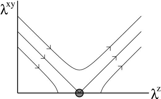
Figure 2: RG flows of Eq. 6.

The effects of Eq. 2 can be deduced by a renormalization group (RG) analysis. More generally, we will consider

$$H_{\rm int} = t\left(\tau^{+}\sigma^{-}_{i,j}\psi^{\dagger}_{i,s}(0)\psi^{\phantom{\dagger}}_{j,s}(0)+h.c.\right)$$ (5)

$$+ t^{\prime}~{}\tau^{z}\sigma^{z}_{i,j}\psi^{\dagger}_{i,s}(0)\psi^{\phantom{\dagger}}_{j,s}(0)-h\tau^{z}\,.$$

Though the $t^{\prime}$ term is not present in Eq. 2, it will be generated upon renormalization. To lowest non-trivial order, the RG equations for the parameters are

$$\frac{d\lambda^{xy}}{dl}=\frac{1}{2}\left(1-\frac{1}{K}\right)\lambda^{xy}+\frac{1}{K}\lambda^{xy}\lambda^{z}\ \ \frac{d\lambda^{z}}{dl}=\left(\lambda^{xy}\right)^{2}\,,$$ , (6)

$$\frac{d\lambda^{h}}{dl}=\lambda^{h}-K(\lambda^{xy})^{2}\lambda^{h}\,.$$

where $\lambda^{xy}\sim t$, $\lambda^{z}\sim t^{\prime}$, and $\lambda^{h}\sim h$. The RG flows in the $\lambda^{z}-\lambda^{xy}$-plane are plotted in Fig. 2. Notice that there is a critical point occurring when $\lambda^{xy}_{c}\equiv(1-K)/(2\sqrt{K})$. For $\lambda^{xy}\leq\lambda^{xy}_{c}$ the coupling flows to zero, while for $\lambda^{xy}>\lambda^{xy}_{c}$ the system flows to strong coupling. Since this critical point arises in the same way as in the pseudogap Kondo model, we will refer to it as the pseudogap Kondo critical point.model For $\lambda^{xy}\leq\lambda^{xy}_{c}$, the system flows to the fixed point where the dot is decoupled from the reservoir. (We will refer to this as the decoupled fixed point.) In terms of the effective Kondo model, the “impurity” is unscreened at low energies. For $\lambda^{xy}>\lambda^{xy}_{c}$, $\lambda^{xy}$ initially decreases under the RG. However, it will eventually start to increase and then flow off to strong coupling. Integrating Eq. 6, we find that $\lambda^{xy}={\cal O}(1)$ at a scale

$$T_{K}=E_{c}\exp\left[\frac{-1}{|\delta|}\left[{\rm arccos}(|\delta|)-{\rm arctan}(x_{0}/|\delta|)\right]\right]\,,$$ (7)

where $x_{0}=(K-1)/(2K)$ and $|\delta|=\sqrt{(\lambda^{xy})^{2}/K-x_{0}^{2}}$. For energies below $T_{K}$, the dot and the reservoir are strongly coupled. The strong coupling fixed point which arises is non-trivial — it corresponds to the 2-channel Kondo fixed point with a spin-1/2 impurity.matveev2 This occurs because both spin-up and spin-down electrons in the reservoir try to occupy the single available charge state on the dot.

It should be noted that a related system was considered recently in Ref. akira, . In that work, the authors considered a resonant level coupled to a Luttinger liquid of spinless fermions. If the Luttinger parameter was smaller than some critical value, $K<K_{c}$, they too found a transition as one tuned the coupling between the dot and the Luttinger liquid. The authors of Ref. akira, focussed on the zero temperature properties of their system. In this work, we show that much rich physics can be observed at finite temperatures and frequencies.

The quantity of experimental interest is the differential capacitance. In terms of the effective Kondo model, this corresponds to the impurity susceptibility. matveev1 ; matveev2 Hence, we will need to calculate correlation functions of impurity operators. To begin with, we will focus on the regime where $\lambda^{xy}<{\cal O}(1)$. In this regime, we can calculate the impurity susceptibility using the RG. In general, an N-point impurity correlation function $G_{N}(\tau_{1},\cdots\tau_{N};\lambda_{i},E_{c})\equiv\langle\tau^{z}(\tau_{1})\cdots\tau^{z}(\tau_{N})\rangle$ satisfies the RG equation

$$\left[\frac{\partial}{\partial l}+\sum_{i}\beta_{i}\frac{\partial}{\partial\lambda_{i}}+N\gamma\right]G_{N}(\tau_{1},\cdots\tau_{N};\lambda_{i},E_{c})=0\,,$$ (8)

where $\beta_{i}=d\lambda_{i}/dl$, and $\gamma$ is the anomalous exponent. The solution of Eq. 8 is

$$G_{N}(\tau_{1},\cdots\tau_{N};\lambda_{i},E_{c})=\exp\left[-N\int_{0}^{l^{*}}dl~{}\gamma(l)\right]$$

$$\hskip 68.65627pt\times G_{N}(\tau_{1},\cdots\tau_{N};\lambda_{i}(l^{*}),e^{-l^{*}}E_{c})\,.$$

Using Eq. 6, we obtain

$$G_{N}(\tau_{1},\cdots\tau_{N};\lambda_{i},E_{c})=e^{-NK(1-K)/2}e^{-NK^{2}f(l^{*})}$$

$$\hskip 54.2025pt\times G_{N}(\tau_{1},\cdots\tau_{N};\lambda_{i}(l^{*}),e^{-l^{*}}E_{c})\,,$$ (9)

where

$$f(l^{*}) = |\delta|\left[\frac{y_{0}^{2}+(|\delta|-x_{0})^{2}e^{2|\delta|l^{*}}}{y_{0}^{2}-(|\delta|-x_{0})^{2}e^{2|\delta|l^{*}}}\right]\ (\lambda^{xy}<\lambda^{xy}_{c})$$ (10a)

$$f(l^{*}) = \frac{x_{0}}{1-x_{0}~{}l^{*}}\ \ \ \ \ (\lambda^{xy}=\lambda^{xy}_{c})$$ (10b)

$$f(l^{*}) = |\delta|\tan\left[|\delta|~{}l^{*}+{\rm arctan}\left(\frac{x_{0}}{|\delta|}\right)\right]\ (\lambda^{xy}>\lambda^{xy}_{c})\,.$$

In Eq. 10, $x_{0}=(K-1)/(2K)$; $y_{0}=\lambda^{xy}/\sqrt{K}$ and $|\delta|=\sqrt{x_{0}^{2}-y_{0}^{2}}$ in Eq. 10a; $|\delta|=\sqrt{(\lambda^{xy})^{2}/K-x_{0}^{2}}$ in Eq. LABEL:RGsolutionc. Choosing $e^{l^{*}}\sim E_{c}/E$, the correlation function on the right-hand-side of Eq. 9 can be evaluated perturbatively.

Figure 3: $C(h;T=0)$ vs. $h$ for $\lambda^{xy}\leq\lambda^{xy}_{c}$ (with $K=0.6$). Solid line: $|\delta|=0$; dashed line: $|\delta|=0.1$; dash-dotted line: $|\delta|=0.2$; dotted line: $|\delta|=0.3$.

We start by considering the temperature dependence of the differential capacitance on resonance, $C(h\rightarrow 0;T)$. Using Eq. 9 with $N=2$, we obtain

$$C(h\rightarrow 0;T)=\frac{e^{K(K-1)}}{4T}~{}e^{-2K^{2}f(T)}\,,$$ (11)

where $f(T)$ is given by Eq. 10 with $l^{*}=\ln(E_{C}/c_{1}T)$. ($c_{1}$ is an ${\cal O}(1)$ constant.) From Eq. 11, we see that $C(h\rightarrow 0;T)\sim T^{-1}$ near the decoupled fixed point ($T\rightarrow 0$ for $\lambda^{xy}\leq\lambda^{xy}_{c}$). Moreover, near the pseudogap Kondo critical point ($\lambda^{xy}=\lambda^{xy}_{c}$ for $T\gg E_{c}\exp[2K/(K-1)]$) $C(h\rightarrow 0;T)\sim T^{\Delta_{T}-1}$ where $\Delta_{T}=(1-K)^{2}/2$. It is also interesting to consider the differential capacitance at $T=0$ as a function of gate voltage, $C(h;T=0)=E_{c}~{}d\langle\tau^{z}\rangle/dh$. Using Eq. 9 with $N=1$, we obtain

$$\langle\tau^{z}\rangle=\pm\frac{e^{K(K-1)/2}}{2}e^{-K^{2}f(|h|)}\,,$$ (12)

where the plus (minus) sign is for $h>0$ ($h<0$), and $f(|h|)$ is given by Eq. 10 with $l^{*}=\ln(E_{C}/c_{2}|h|)$. ($c_{2}$ is another ${\cal O}(1)$ constant.) The differential capacitance vs. gate voltage is plotted in Fig. 3. Near the decoupled fixed point, we find $C(h;T=0)\sim|h|^{2|\delta|-1}$ as $|h|\rightarrow 0$ ($|\delta|$ is as in Eq. 10a). Also, near the pseudogap Kondo critical point $C(h;T=0)\sim|h|^{\Delta_{h}-1}$ where $\Delta_{h}=(1-K)^{2}/4$ ($|h|\gg E_{c}\exp[2K/(K-1)]$).

Notice that near the decoupled fixed point, $C(h\rightarrow 0;T)\sim T^{-1}$ as $T\rightarrow 0$. This Curie-Weiss-like form arises because the “impurity” behaves basically like a free spin. However, the local “moment” is reduced from its non-interacting value.vojta ; konik ; akira From Eqs. 12, we see that the amount by which the local “moment” is reduced depends on $K$, as well as the value of $\lambda^{xy}$. Also, notice that $\Delta_{T}=2\Delta_{h}$ near the pseudogap Kondo critical point. In Ref. si1, , it was shown that the exponents near the critical point of the pseudogap Kondo model satisfy certain hyperscaling relations. To the order of accuracy that we have worked, our results are consistent with these hyperscaling relations.

Now, we consider the physics in the regime $\lambda^{xy}>\lambda^{xy}_{c}$ for energies below $T_{K}$ (with $T_{K}$ given by Eq. 7). In this regime, the system is close to the 2-channel Kondo fixed point. To proceed, we follow Ref. schiller, and form combinations of the fields in the dot and the reservoir: $\phi_{R,c}$, $\phi_{R,sp}$, $\phi_{R,f}$, and $\phi_{R,sf}$. Then, we perform the unitary transformation, $U=\exp\left(i\sqrt{4\pi/K}~{}\tau^{z}\phi_{R,f}(0)\right)$, which ties charge to the “impurity”. Finally, we introduce new fermion fields, $d\sim\tau^{-}$, $X\sim e^{i\sqrt{4\pi}\phi_{R,sf}}$, and $f\sim e^{i\sqrt{4\pi}\phi_{R,f}}$. Upon performing these transformations, $H_{\rm int}$ becomes

$$H_{\rm int} = v_{F}\tilde{\lambda}^{xy}\left(d^{\dagger}+d~{}\right)\left(X^{\dagger}(0)-X(0)\right)$$ (13)

$$+ v_{F}\sqrt{4\pi/K}\left(\tilde{\lambda}^{z}-1\right)\left(d^{\dagger}d^{\phantom{\dagger}}-1/2\right)f^{\dagger}(0)f(0)$$

$$- v_{F}\tilde{\lambda}^{h}\left(d^{\dagger}d^{\phantom{\dagger}}-1/2\right)\,,$$

where $\tilde{\lambda}^{xy}$, $\tilde{\lambda}^{z}$, and $\tilde{\lambda}^{h}$ are the renormalized values of the couplings.

Using Eq. 13, we can calculate the differential capacitance near the 2-channel Kondo fixed point. Starting with the differential capacitance on resonance, we find (ignoring the irrelevant $(\tilde{\lambda}^{z}-1)$ term)

$$C(h\rightarrow 0;\omega,T)=$$ (14)

$$\hskip 14.45377pt\frac{1}{T_{K}}\int\frac{dx}{2\pi}{\rm tanh}\left(\frac{xT_{K}}{2T}\right)\frac{1}{x^{2}+1}\frac{1}{x-(\omega/T_{K})-i0^{+}}\,,$$

For $\omega=0$ and $T\ll T_{K}$, this reduces to the well-known result for the impurity susceptibility of the 2-channel Kondo model $C(h\rightarrow 0;T)=1/(\pi T_{K})\ln(T_{K}/T)$. We can also calculate $C(h;T=0)$. Using Eq. 13 (ignoring the irrelevant $(\tilde{\lambda}^{z}-1)$ term)

$$\langle\tau^{z}\rangle=\frac{h}{T_{K}}\int\frac{dx}{2\pi}{\rm tanh}\left(\frac{xT_{K}}{2T}\right)\frac{x}{(x^{2}-(h/T_{K})^{2})^{2}+x^{2}}\,.$$ (15)

For $T=0$ and $|h|\ll T_{K}$, $C(h;T=0)=4/(\pi T_{K})\ln(T_{K}/|h|)$. Notice that $C(h\rightarrow 0;T)$ ($C(h;T=0)$) diverges as $T\rightarrow 0$ ($|h|\rightarrow 0$). However, the divergence in this case is weaker than what occurs near the decoupled fixed point. This is because, near the 2-channel Kondo fixed point, charge is tied to the “impurity”. As a result, the ground states $\tau^{z}=1/2$ and $\tau^{z}=-1/2$ are orthogonal, in that they are not connected by $\tau^{+}$ or $\tau^{-}$.giamarchi This removes the power-law divergence which occurs near the decoupled fixed point, and replaces it with the weaker logarithmic divergence.

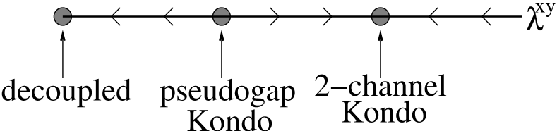
Figure 4: Fixed points and RG flows for the pseudogap Kondo model.

In the above discussion, we saw three fixed points arise (shown schematically in Fig. 4): (1) the decoupled fixed point, (2) the pseudogap Kondo critical point, and (3) the 2-channel Kondo fixed point. The pseudogap Kondo critical point and the 2-channel Kondo fixed points are particularly interesting because they are non-trivial scale invariant fixed points. As a consequence, one should be able to observe $\omega/T$-scaling near these fixed points by applying an AC component to the gate voltage. More specifically, we expect the dynamical capacitance on resonance to have the form

$$C(h\rightarrow 0;\omega,T)=T^{\nu-1}X(\omega/T)\,.$$ (16)

Near the pseudogap Kondo critical point, we can calculate the scaling function $X(\omega/T)$ for $(1-K)\ll 1$. In the leading logarithm approximation, we find $\nu=\Delta_{T}$ ($\Delta_{T}=(1-K)^{2}/2$) and

$$X(\omega/T)=\frac{1}{4\pi}\left(\frac{2\pi}{E_{c}}\right)^{\nu}\sin\left(\frac{\pi\nu}{2}\right)B\left(\frac{\nu}{2}-i\frac{\omega}{2\pi T},1-\nu\right)$$

where $B$ is the beta function. Near the 2-channel Kondo fixed point, we use Eq. 14 to obtain $\nu=1$ and

$$X(\omega/T)=\frac{1}{\pi T_{K}}\ln\left(\frac{T_{K}}{{\rm max}(\omega,T)}\right)+\frac{i}{2T_{K}}~{}{\rm tanh}\left(\frac{\omega}{2T}\right)\,.$$

Note that $X(\omega/T)$ is, in general, complex. Therefore, the differential capacitance will have components both in-phase and out-of-phase with the gate voltage.

To summarize, a (large) quantum dot coupled to an interacting one-dimensional electron liquid could provide a controlled environment to observe pseudogap Kondo physics. By tuning the coupling between the dot and the one-dimensional electron liquid, one can access the various fixed points which arise: the decoupled fixed point, the pseudogap Kondo critical point, and the 2-channel Kondo fixed point. Moreover, this system provides the remarkable opportunity to directly probe impurity properties via differential capacitance measurements. As the differential capacitance of a large quantum dot has recently been measured,ashoori we are hopeful that the physics described in this work can be observed in the near future.

We would like to thank G. Sierra and A. Furusaki for very helpful discussions. This work was supported by the NSERC of Canada (EHK, YBK, CK), Materials and Manufacturing of Ontario (EHK, YBK, CK), Canada Research Chair (YBK), and Alfred P. Sloan Foundation (YBK).

References

• (1) For a review, see L. Kouwenhoven and L. Glazman, Physics World 14(1), 33 (2001).
• (2) D. Withoff and E. Fradkin, Phys. Rev. Lett. 64, 1835 (1990).
• (3) A. Polkovnikov, S. Sachdev, and M. Vojta, Phys. Rev. Lett. 86, 296 (2001); M. Vojta and R. Bulla, Phys. Rev. B 65, 014511 (2002).
• (4) Q. Si, et. al., Nature 413, 804 (2001).
• (5) K. Ingersent and Q. Si, cond-mat/0109417.
• (6) K.Β A. Matveev, Sov. Phys. JETP 72, 892 (1991).
• (7) E.Β B. Kolomeisky, R.Β M. Konik, and X. Qi, cond-mat/0203573.
• (8) C. de C. Chamon and E. Fradkin, Phys. Rev. B 56, 2012 (1997).
• (9) S. Eggert and I. Affleck, Phys. Rev. B 46, 10866 (1992).
• (10) Our model is not identical to the pseudogap Kondo model. In the pseudogap Kondo model, the $x$, $y$, and $z$ components of the Kondo interaction scale in the same way. In our model, the $x$ and $y$ components scale differently from the $z$ component. (See Eq.Β 6.)
• (11) K.Β A. Matveev, Phys. Rev. B 51, 1743 (1995).
• (12) A. Furusaki and K.Β A. Matveev, cond-mat/0112426.
• (13) M. Vojta, Phys. Rev. Lett. 87, 097202 (2001); C. Gonzalez-Buxton and K. Ingersent, Phys. Rev. B 57, 14254 (1998).
• (14) A. Schiller and S. Hershfield, Phys. Rev. B 51, R12896 (1995); K. Majumdar, A. Schiller, and S. Hershfield, ibid 57, 2991 (1998).
• (15) D.Β G. Clarke, T. Giamarchi, and B.Β I. Shraiman, Phys. Rev. B 48, 7070 (1993).
• (16) D. Berman, et. al., Phys. Rev. Lett. 82, 161 (1999).