The spread of epidemic disease on networks

Abstract

The study of social networks, and in particular the spread of disease on networks, has attracted considerable recent attention in the physics community. In this paper, we show that a large class of standard epidemiological models, the so-called susceptible/infective/removed (SIR) models can be solved exactly on a wide variety of networks. In addition to the standard but unrealistic case of fixed infectiveness time and fixed and uncorrelated probability of transmission between all pairs of individuals, we solve cases in which times and probabilities are non-uniform and correlated. We also consider one simple case of an epidemic in a structured population, that of a sexually transmitted disease in a population divided into men and women. We confirm the correctness of our exact solutions with numerical simulations of SIR epidemics on networks.

I Introduction

Many diseases spread through human populations by contact between infective individuals (those carrying the disease) and susceptible individuals (those who do not have the disease yet, but can catch it). The pattern of these disease-causing contacts forms a network. In this paper we investigate the effect of network topology on the rate and pattern of disease spread.

Most mathematical studies of disease propagation make the assumption that populations are “fully mixed,” meaning that an infective individual is equally likely to spread the disease to any other member of the population or subpopulation to which they belong Bailey75 ; AM91 ; Hethcote00 . In the limit of large population size this assumption allows one to write down nonlinear differential equations governing, for example, numbers of infective individuals as a function of time, from which solutions for quantities of interest can be derived, such as typical sizes of outbreaks and whether or not epidemics occur. (Epidemics are defined as outbreaks that affect a non-zero fraction of the population in the limit of large system size.) Epidemic behavior usually shows a phase transition with the parameters of the model—a sudden transition from a regime without epidemics to one with. This transition happens as the “reproductive ratio” $R_{0}$ of the disease, which is the fractional increase per unit time in the number of infective individuals, passes though one.

Within the class of fully mixed models much elaboration is possible, particularly concerning the effects of age structure in the population, and population turnover. The crucial element however that all such models lack is network topology. It is obvious that a given infective individual does not have equal probability of infecting all others; in the real world each individual only has contact with a small fraction of the total population, although the number of contacts that people have can vary greatly from one person to another. The fully mixed approximation is made primarily in order to allow the modeler to write down differential equations. For most diseases it is not an accurate representation of real contact patterns.

In recent years a large body of research, particularly within the statistical physics community, has addressed the topological properties of networks of various kinds, from both theoretical and empirical points of view, and studied the effects of topology on processes taking place on those networks Strogatz01 ; AB02 . Social networks WS98 ; ASBS00 ; Liljeros01 ; GN02 , technological networks ABW98 ; AJB99 ; FFF99 ; Broder00 , and biological networks Jeong00 ; Jeong01 ; FW00 ; WM00 ; MS02 have all been examined and modeled in some detail. Building on insights gained from this work, a number of authors have pursued a mathematical theory of the spread of disease on networks MN00a ; KA01 ; PV01a ; MPV02 ; WSS01 ; Warren02 . This is also the topic of the present paper, in which we show that a large class of standard epidemiological models can be solved exactly on networks using ideas drawn from percolation theory.

The outline of the paper is as follows. In Section II we introduce the models studied. In Section III we show how percolation ideas and generating function methods can be used to provide exact solutions of these models on simple networks with uncorrelated transmission probabilities. In Section IV we extend these solutions to cases in which probabilities of transmission are correlated, and in Section V to networks representing some types of structured populations. In Section VI we give our conclusions.

II Epidemic models and percolation

The mostly widely studied class of epidemic models, and the one on which we focus in this paper, is the class of susceptible/infective/removed or SIR models. The original and simplest SIR model, first formulated (though never published) by Lowell Reed and Wade Hampton Frost in the 1920s, is as follows. A population of $N$ individuals is divided into three states: susceptible (S), infective (I), and removed (R). In this context “removed” means individuals who are either recovered from the disease and immune to further infection, or dead. (Some researchers consider the R to stand for “recovered” or “refractory.” Either way, the meaning is the same.) Infective individuals have contacts with randomly chosen individuals of all states at an average rate $\beta$ per unit time, and recover and acquire immunity (or die) at an average rate $\gamma$ per unit time. If those with whom infective individuals have contact are themselves in the susceptible state, then they become infected. In the limit of large $N$ this model is governed by the coupled nonlinear differential equations Bailey75 :

$${{\rm d}s\over{\rm d}t}=-\beta is,\quad{{\rm d}i\over{\rm d}t}=\beta is-\gamma i,\quad{{\rm d}r\over{\rm d}t}=\gamma i,$$ (1)

where $s(t)$, $i(t)$, and $r(t)$ are the fractions of the population in each of the three states, and the last equation is redundant, since necessarily $s+i+r=1$ at all times. This model is appropriate for a rapidly spreading disease that confers immunity on its survivors, such as influenza. In this article we will consider only diseases of this type. Diseases that are endemic because they propagate on timescales comparable to or slower than the rate of turnover of the population, or because they confer only temporary immunity, are not well represented by this model; other models have been developed for these cases Hethcote00 .

The model described above assumes that the population is fully mixed, meaning that the individuals with whom a susceptible individual has contact are chosen at random from the whole population. It also assumes that all individuals have approximately the same number of contacts in the same time, and that all contacts transmit the disease with the same probability. In real life none of these assumptions is correct, and they are all grossly inaccurate in at least some cases. In the work presented here we remove these assumptions by a series of modifications of the model.

First, as many others have done, we replace the “fully mixed” aspect with a network of connections between individuals MN00a ; KA01 ; PV01a ; WSS01 ; Warren02 ; MPV02 ; SS88 ; Longini88 ; KM96 ; BMS97 . Individuals have disease-causing contacts only along the links in this network. We distinguish here between “connections” and actual contacts. Connections between pairs of individuals predispose those individuals to disease-causing contact, but do not guarantee it. An individual’s connections are the set of people with whom the individual may have contact during the time he or she is infective—people that the individual lives with, works with, sits next to on the bus, and so forth.

We can vary the number of connections each person has with others by choosing a particular degree distribution for the network. (Recall that the degree of a vertex in a network is the number of other vertices to which it is attached.) For example, in the case of sexual contacts, which can transmit STDs, the degree distribution has been found to follow a power-law form Liljeros01 . By placing the model on a network with a power-law degree distribution we can emulate this effect in our model.

Our second modification of the model is to allow the probability of disease-causing contact between pairs of individuals who have a connection to vary, so that some pairs have higher probability of disease transmission than others.

Consider a pair of individuals who are connected, one of whom $i$ is infective and the other $j$ susceptible. Suppose that the average rate of disease-causing contacts between them is $r_{ij}$, and that the infective individual remains infective for a time $\tau_{i}$. Then the probability $1-T_{ij}$ that the disease will not be transmitted from $i$ to $j$ is

$$1-T_{ij}=\lim_{\delta t\to 0}(1-r_{ij}\delta t)^{\tau_{i}/\delta t}={\rm e}^{-r_{ij}\tau_{i}},$$ (2)

and the probability of transmission is

$$T_{ij}=1-{\rm e}^{-r_{ij}\tau_{i}}.$$ (3)

Some models, particularly computer simulations, use discrete time-steps rather than continuous time, in which case instead of taking the limit in Eq. (2) we simply set $\delta t=1$, giving

$$T_{ij}=1-(1-r_{ij})^{\tau_{i}},$$ (4)

where $\tau$ is measured in time-steps.

In general $r_{ij}$ and $\tau_{i}$ will vary between individuals, so that the probability of transmission also varies. Let us assume initially that these two quantities are iid random variables chosen from some appropriate distributions $P(r)$ and $P(\tau)$. (We will relax this assumption later.) The rate $r_{ij}$ need not be symmetric—the probability of transmission in either direction might not be the same. In any case, $T_{ij}$ is in general not symmetric because of the appearance of $\tau_{i}$ in Eqs. (3) and (4).

Now here’s the trick: because $r_{ij}$ and $\tau_{i}$ are iid random variables, so is $T_{ij}$, and hence the a priori probability of transmission of the disease between two individuals is simply the average $T$ of $T_{ij}$ over the distributions $P(r)$ and $P(\tau)$, which is

$$T=\left\langle T_{ij}\right\rangle=1-\int_{0}^{\infty}{\rm d}r\>{\rm d}\tau\>P(r)P(\tau)\,{\rm e}^{-r\tau}$$ (5)

for the continuous time case or

$$T=1-\int_{0}^{\infty}{\rm d}r\>\sum_{\tau=0}^{\infty}\>P(r)P(\tau)\,(1-r)^{\tau}$$ (6)

for the discrete case WSS01 . We call $T$ the “transmissibility” of the disease. It is necessarily always in the range $0\leq T\leq 1$.

Thus the fact that individual transmission probabilities vary makes no difference whatsoever; in the population as a whole the disease will propagate as if all transmission probabilities were equal to $T$. We demonstrate the truth of this result by explicit simulation in Section III.5. It is this result that makes our models solvable. Cases in which the variables $r$ and $\tau$ are not iid are trickier, but, as we will show, these are sometimes solvable as well.

We note further that more complex disease transmission models, such as SEIR models in which there is an infected-but-not-infective period (E), are also covered by this formalism. The transmissibility $T_{ij}$ is essentially just the integrated probability of transmission of the disease between two individuals. The precise temporal behavior of infectivity and other variables is unimportant. Indeed the model can be generalized to include any temporal variation in infectivity of the infective individuals, and transmission can still be represented correctly by a simple transmissibility variable $T$, as above.

Now imagine watching an outbreak of the disease, which starts with a single infective individual, spreading across our network. If we were to mark or “occupy” each edge in the graph across which the disease is transmitted, which happens with probability $T$, the ultimate size of the outbreak would be precisely the size of the cluster of vertices that can be reached from the initial vertex by traversing only occupied edges. Thus, the model is precisely equivalent to a bond percolation model with bond occupation probability $T$ on the graph representing the community. The connection between the spread of disease and percolation was in fact one of the original motivations for the percolation model itself FH63 , but seems to have been formulated in the manner presented here first by Grassberger Grassberger83 for the case of uniform $r$ and $\tau$, and by Warren et al. WSS01 ; Warren02 for the non-uniform case.

In the next section we show how the percolation problem can be solved on random graphs with arbitrary degree distributions, giving exact solutions for the typical size of outbreaks, presence of an epidemic, size of the epidemic (if there is one), and a number of other quantities of interest.

III Exact solutions on networks with arbitrary degree distributions

One of the most important results to come out of empirical work on networks is the finding that the degree distributions of many networks are highly right-skewed. In other words, most vertices have only a low degree, but there are a small number whose degree is very high Price65 ; AJB99 ; ASBS00 ; AB02 . The network of sexual contacts discussed above provides one example of such a distribution Liljeros01 . It is known that the presence of highly connected vertices can have a disproportionate effect on certain properties of the network. Recent work suggests that the same may be true for disease propagation on networks PV01a ; LM01 , and so it will be important that we incorporate non-trivial degree distributions in our models. As a first illustration of our method therefore, we look at a simple class of unipartite graphs studied previously by a variety of authors BC78 ; MR95 ; MR98 ; NSW01 ; NWS02 ; CEBH00 ; CEBH01 ; CNSW00 ; DMS01a ; ALPH01 , in which the degree distribution is specified, but the graph is in other respects random.

Our graphs are simply defined. One specifies the degree distribution by giving the properly normalized probabilities $p_{k}$ that a randomly chosen vertex has degree $k$. A set of $N$ degrees $\left\{k_{i}\right\}$, also called a degree sequence, is then drawn from this distribution and each of the $N$ vertices in the graph is given the appropriate number $k_{i}$ of “stubs”—ends of edges emerging from it. Pairs of these stubs are then chosen at random and connected together to form complete edges. Pairing of stubs continues until none are left. (If an odd number of stubs is by chance generated, complete pairing is not possible, in which case we discard one $k_{i}$ and draw another until an even number is achieved.) This technique guarantees that the graph generated is chosen uniformly at random from the set of all graphs with the selected degree sequence.

All the results given in this section are averaged over the ensemble of possible graphs generated in this way, in the limit of large graph size.

III.1 Generating functions

We wish then to solve for the average behavior of graphs of this type under bond percolation with bond occupation probability $T$. We will do this using generating function techniques Wilf94 . Following Newman et al. NSW01 , we define a generating function for the degree distribution thus:

$$G_{0}(x)=\sum_{k=0}^{\infty}p_{k}x^{k}.$$ (7)

Note that $G_{0}(1)=\sum_{k}p_{k}=1$ if $p_{k}$ is a properly normalized probability distribution.

This function encapsulates all of the information about the degree distribution. Given it, we can easily reconstruct the distribution by repeated differentiation:

$$p_{k}={1\over k!}{{\rm d}^{k}G_{0}\over{\rm d}x^{k}}\bigg{|}_{x=0}.$$ (8)

We say that the generating function $G_{0}$ “generates” the distribution $p_{k}$. The generating function is easier to work with than the degree distribution itself because of two crucial properties:

Powers If the distribution of a property $k$ of an object is generated by a given generating function, then the distribution of the sum of $k$ over $m$ independent realizations of the object is generated by the $m^{\rm th}$ power of that generating function. For example, if we choose $m$ vertices at random from a large graph, then the distribution of the sum of the degrees of those vertices is generated by $[G_{0}(x)]^{m}$.

Moments The mean of the probability distribution generated by a generating function is given by the first derivative of the generating function, evaluated at 1. For instance, the mean degree $z$ of a vertex in our network is given by

$$z=\left\langle k\right\rangle=\sum_{k}kp_{k}=G_{0}^{\prime}(1).$$ (9)

Higher moments of the distribution can be calculated from higher derivatives also. In general, we have

$$\left\langle k^{n}\right\rangle=\sum_{k}k^{n}p_{k}=\biggl{[}\biggl{(}x{{\rm d}\over{\rm d}x}\biggr{)}^{\!n}G_{0}(x)\biggr{]}_{x=1}.$$ (10)

A further observation that will also prove crucial is the following. While $G_{0}$ above correctly generates the distribution of degrees of randomly chosen vertices in our graph, a different generating function is needed for the distribution of the degrees of vertices reached by following a randomly chosen edge. If we follow an edge to the vertex at one of its ends, then that vertex is more likely to be of high degree than is a randomly chosen vertex, since high-degree vertices have more edges attached to them than low-degree ones. The distribution of degrees of the vertices reached by following edges is proportional to $kp_{k}$, and hence the generating function for those degrees is

$${\sum_{k}kp_{k}x^{k}\over\sum_{k}kp_{k}}=x{G_{0}^{\prime}(x)\over G_{0}^{\prime}(1)}.$$ (11)

In general we will be concerned with the number of ways of leaving such a vertex excluding the edge we arrived along, which is the degree minus 1. To allow for this, we simply divide the function above by one power of $x$, thus arriving at a new generating function

$$G_{1}(x)={G_{0}^{\prime}(x)\over G_{0}^{\prime}(1)}={1\over z}\,G_{0}^{\prime}(x),$$ (12)

where $z$ is the average vertex degree, as before.

In order to solve the percolation problem, we will also need generating functions $G_{0}(x;T)$ and $G_{1}(x;T)$ for the distribution of the number of occupied edges attached to a vertex, as a function of the transmissibility $T$. These are simple to derive. The probability of a vertex having exactly $m$ of the $k$ edges emerging from it occupied is given by the binomial distribution ${k\choose m}T^{m}(1-T)^{k-m}$, and hence the probability distribution of $m$ is generated by

$$G_{0}(x;T) = \sum_{m=0}^{\infty}\sum_{k=m}^{\infty}p_{k}\biggl{(}{k\atop m}\biggr{)}T^{m}(1-T)^{k-m}x^{m}$$ (13)

$$= \sum_{k=0}^{\infty}p_{k}\sum_{m=0}^{k}\biggl{(}{k\atop m}\biggr{)}(xT)^{m}(1-T)^{k-m}$$

$$= \sum_{k=0}^{\infty}p_{k}(1-T+xT)^{k}$$

$$= G_{0}(1+(x-1)T).$$

Similarly, the probability distribution of occupied edges leaving a vertex arrived at by following a randomly chosen edge is generated by

$$G_{1}(x;T)=G_{1}(1+(x-1)T).$$ (14)

Note that, in our notation

$$G_{0}(x;1) = G_{0}(x),$$ (15a)

$$G_{0}(1;T) = G_{0}(1),$$ (15b)

$$G_{0}^{\prime}(1;T) = TG_{0}^{\prime}(1),$$ (15c)

and similarly for $G_{1}$. ($G_{0}^{\prime}(x;T)$ here represents the derivative of $G_{0}(x;T)$ with respect to its first argument.)

III.2 Outbreak size distribution

The first quantity we will work out is the distribution $P_{s}(T)$ of the sizes $s$ of outbreaks of the disease on our network, which is also the distribution of sizes of clusters of vertices connected together by occupied edges in the corresponding percolation model. Let $H_{0}(x;T)$ be the generating function for this distribution:

$$H_{0}(x;T)=\sum_{s=0}^{\infty}P_{s}(T)x^{s}.$$ (16)

By analogy with the previous section we also define $H_{1}(x;T)$ to be the generating function for the cluster of connected vertices we reach by following a randomly chosen edge.

Now, following Ref. NSW01, , we observe that $H_{1}$ can be broken down into an additive set of contributions as follows. The cluster reached by following an edge may be:

1. a single vertex with no occupied edges attached to it, other than the one along which we passed in order to reach it;

2. a single vertex attached to any number $m\geq 1$ of occupied edges other than the one we reached it by, each leading to another cluster whose size distribution is also generated by $H_{1}$.

We further note that the chance that any two finite clusters that are attached to the same vertex will have an edge connecting them together directly goes as $N^{-1}$ with the size $N$ of the graph, and hence is zero in the limit $N\to\infty$. In other words, there are no loops in our clusters; their structure is entirely tree-like.

Using these results, we can express $H_{1}(x;T)$ in a Dyson-equation-like self-consistent form thus:

$$H_{1}(x;T)=xG_{1}(H_{1}(x;T);T).$$ (17)

Then the size of the cluster reachable from a randomly chosen starting vertex is distributed according to

$$H_{0}(x;T)=xG_{0}(H_{1}(x;T);T).$$ (18)

It is straightforward to verify that for the special case $T=1$ of 100% transmissibility, these equations reduce to those given in Ref. NSW01, for component size in random graphs with arbitrary degree distributions. Equations (17) and (18) provide the solution for the more general case of finite transmissibility which applies to SIR models. Once we have $H_{0}(x;T)$, we can extract the probability distribution of clusters $P_{s}(T)$ by differentiation using Eq. (8) on $H_{0}$. In most cases however it is not possible to find arbitrary derivatives of $H_{0}$ in closed form. Instead we typically evaluate them numerically. Since direct evaluation of numerical derivatives is prone to machine precision problems, we recommend evaluating the derivatives by numerical contour integration using the Cauchy formula:

$$P_{s}(T)={1\over s!}\,{{\rm d}^{s}\!H_{0}\over{\rm d}x^{s}}\bigg{|}_{x=0}={1\over 2\pi{\rm i}}\oint{H_{0}(\zeta;T)\over\zeta^{s+1}}{\rm d}\zeta,$$ (19)

where the integral is over the unit circle MN00b . It is possible to find the first thousand derivatives of a function without difficulty using this method NSW01 . By this method then, we can find the exact probability $P_{s}$ that a particular outbreak of our disease will infect $s$ people in total, as a function of the transmissibility $T$.

III.3 Outbreak sizes and the epidemic transition

Although in general we must use numerical methods to find the complete distribution $P_{s}$ of outbreak sizes from Eq. (19), we can find the mean outbreak size in closed form. Using Eq. (9), we have

$$\left\langle s\right\rangle=H_{0}^{\prime}(1;T)=1+G_{0}^{\prime}(1;T)H_{1}^{\prime}(1;T),$$ (20)

where we have made use of the fact that the generating functions are 1 at $x=1$ if the distributions that they generate are properly normalized. Differentiating Eq. (17), we have

$$H_{1}^{\prime}(1;T)=1+G_{1}^{\prime}(1;T)H_{1}^{\prime}(1;T)={1\over 1-G_{1}^{\prime}(1;T)},$$ (21)

and hence

$$\left\langle s\right\rangle=1+{G_{0}^{\prime}(1;T)\over 1-G_{1}^{\prime}(1;T)}=1+{TG_{0}^{\prime}(1)\over 1-TG_{1}^{\prime}(1)}.$$ (22)

Given Eqs. (7), (12), (13), and (14), we can then evaluate this expression to get the mean outbreak size for any value of $T$ and degree distribution.

We note that Eq. (22) diverges when $TG_{1}^{\prime}(1)=1$. This point marks the onset of an epidemic; it is the point at which the typical outbreak ceases to be confined to a finite number of individuals, and expands to fill an extensive fraction of the graph. The transition takes place when $T$ is equal to the critical transmissibility $T_{c}$, given by

$$T_{c}={1\over G_{1}^{\prime}(1)}={G_{0}^{\prime}(1)\over G_{0}^{\prime\prime}(1)}={\sum_{k}kp_{k}\over\sum_{k}k(k-1)p_{k}}.$$ (23)

For $T>T_{c}$, we have an epidemic, or “giant component” in the language of percolation. We can calculate the size of this epidemic as follows. Above the epidemic threshold Eq. (17) is no longer valid because the giant component is extensive and therefore can contain loops, which destroys the assumptions on which Eq. (17) was based. The equation is valid however if we redefine $H_{0}$ to be the generating function only for outbreaks other than epidemic outbreaks, i.e., isolated clusters of vertices that are not connected to the giant component. These however do not fill the entire graph, but only the portion of it not affected by the epidemic. Thus, above the epidemic transition, we have

$$H_{0}(1;T)=\sum_{s}P_{s}=1-S(T),$$ (24)

where $S(T)$ is the fraction of the population affected by the epidemic. Rearranging Eq. (24) for $S$ and making use of Eq. (18), we find that the size of the epidemic is

$$S(T)=1-G_{0}(u;T),$$ (25)

where $u\equiv H_{1}(1;T)$ is the solution of the self-consistency relation

$$u=G_{1}(u;T).$$ (26)

Results equivalent to Eqs. (22) to (26) were given previously in a different context in Ref. CNSW00, .

Note that it is not the case, even above $T_{c}$, that all outbreaks give rise to epidemics of the disease. There are still finite outbreaks even in the epidemic regime. While this appears very natural, it stands nonetheless in contrast to the standard fully mixed models, for which all outbreaks give rise to epidemics above the epidemic transition point. In the present case, the probability of an outbreak becoming an epidemic at a given $T$ is simply equal to $S(T)$.

III.4 Degree of infected individuals

The quantity $u$ defined in Eq. (26) has a simple interpretation: it is the probability that the vertex at the end of a randomly chosen edge remains uninfected during an epidemic (i.e., that it belongs to one of the finite components). The probability that a vertex becomes infected via one of its edges is thus $v=1-T+Tu$, which is the sum of the probability $1-T$ that the edge is unoccupied, and the probability $Tu$ that it is occupied but connects to an uninfected vertex. The total probability of being uninfected if a vertex has degree $k$ is $v^{k}$, and the probability of having degree $k$ given that a vertex is uninfected is $p_{k}v^{k}/\sum_{k}p_{k}v^{k}=p_{k}v^{k}/G_{0}(v)$, which distribution is generated by the function $G_{0}(vx)/G_{0}(v)$. Differentiating and setting $x=1$, we then find that the average degree $z_{\rm out}$ of vertices outside the giant component is

$$z_{\rm out}={vG_{0}^{\prime}(v)\over G_{0}(v)}={vG_{1}(v)\over G_{0}(v)}\,z={u[1-T+Tu]\over 1-S}\,z.$$ (27)

Similarly the degree distribution for an infected vertex is generated by $[G_{0}(x)-G_{0}(vx)]\big{/}[1-G_{0}(v)]$, which gives a mean degree $z_{\rm in}$ for vertices in the giant component of

$$z_{\rm in}={1-vG_{1}(v)\over 1-G_{0}(v)}\,z={1-u[1-T+Tu]\over S}\,z.$$ (28)

Note that $1-S=G_{0}(u;T)\leq u$, since all coefficients of $G_{0}(x;T)$ are by definition positive (because they form a probability distribution) and hence $G_{0}(x;T)$ has only positive derivatives, meaning that it is convex everywhere on the positive real line within its domain of convergence. Thus, from Eq. (27), $z_{\rm out}\leq z$. Similarly, $z_{\rm in}\geq z$, and hence, as we would expect, the mean degree of infected individuals is always greater than or equal to the mean degree of uninfected ones. Indeed, the probability of a vertex being infected, given that it has degree $k$, goes as $1-v^{k}=1-{\rm e}^{-k\log(1/v)}$, i.e., tends exponentially to unity as degree becomes large.

III.5 An example

Let us now look at an application of these results to a specific example of disease spreading. First of all we need to define our network of connections between individuals, which means choosing a degree distribution. Here we will consider graphs with the degree distribution

$$p_{k}=\biggl{\{}\begin{array}[]{ll}0&\mbox{for $k=0$}\\ Ck^{-\alpha}{\rm e}^{-k/\kappa}\hbox{}&\mbox{for $k\geq 1$.}\end{array}$$ (29)

where $C$, $\alpha$, and $\kappa$ are constants. In other words, the distribution is a power-law of exponent $\alpha$ with an exponential cutoff around degree $\kappa$. This distribution has been studied before by various authors ASBS00 ; NSW01 ; NWS02 ; CNSW00 . It makes a good example for a number of reasons:

1. distributions of this form are seen in a variety of real-world networks ASBS00 ; Newman01a ;

2. it includes pure power-law and pure exponential distributions, both of which are also seen in various networks Price65 ; AJB99 ; FFF99 ; ASBS00 , as special cases when $\kappa\to\infty$ or $\alpha\to 0$;

3. it is normalizable and has all moments finite for any finite $\kappa$;

The constant $C$ is fixed by the requirement of normalization, which gives $C=[\mathop{\rm Li}_{\alpha}({\rm e}^{-1/\kappa})]^{-1}$ and hence

$$p_{k}={k^{-\alpha}{\rm e}^{-k/\kappa}\over\mathop{\rm Li}_{\alpha}({\rm e}^{-1/\kappa})}\qquad\mbox{for $k\geq 1$,}$$ (30)

where $\mathop{\rm Li}_{n}(x)$ is the $n$th polylogarithm of $x$.

We also need to choose the distributions $P(r)$ and $P(\tau)$ for the transmission rate and the time spent in the infective state. For the sake of easier comparison with computer simulations we use discrete time and choose both distributions to be uniform, with $r$ real in the range $0\leq r<r_{\rm max}$ and $\tau$ integer in the range $1\leq\tau\leq\tau_{\rm max}$. The transmissibility $T$ is then given by Eq. (6). From Eq. (30), we have

$$G_{0}(x)={\mathop{\rm Li}_{\alpha}(x{\rm e}^{-1/\kappa})\over\mathop{\rm Li}_{\alpha}({\rm e}^{-1/\kappa})}.$$ (31)

and

$$G_{1}(x)={\mathop{\rm Li}_{\alpha-1}(x{\rm e}^{-1/\kappa})\over x\mathop{\rm Li}_{\alpha-1}({\rm e}^{-1/\kappa})}.$$ (32)

Thus the epidemic transition in this model occurs at

$$T_{c}={\mathop{\rm Li}_{\alpha-1}({\rm e}^{-1/\kappa})\over\mathop{\rm Li}_{\alpha-2}({\rm e}^{-1/\kappa})-\mathop{\rm Li}_{\alpha-1}({\rm e}^{-1/\kappa})}.$$ (33)

Below this value of $T$ there are only small (non-epidemic) outbreaks, which have mean size

$$\left\langle s\right\rangle = 1+$$

$${T[\mathop{\rm Li}_{\alpha-1}({\rm e}^{-1/\kappa})]^{2}\over\mathop{\rm Li}_{\alpha}({\rm e}^{-1/\kappa})[(T+1)\mathop{\rm Li}_{\alpha-1}({\rm e}^{-1/\kappa})-T\mathop{\rm Li}_{\alpha-2}({\rm e}^{-1/\kappa})]}.$$

Above it, we are in the region in which epidemics can occur, and they affect a fraction $S$ of the population in the limit of large graph size. We cannot solve for $S$ in closed form, but we can solve Eqs. (25) and (26) by numerical iteration and hence find $S$.

Figure 1: Epidemic size (top) and average outbreak size (bottom) for the SIR model on networks with degree distributions of the form (30) as a function of transmissibility. Solid lines are the exact solutions, Eqs. (25) and (22), for $\alpha=2$ and (left to right in each panel) $\kappa=20$, 10, and 5. Each of the points is an average result for $10\,000$ simulations on graphs of $100\,000$ vertices each with distributions of $r$ and $\tau$ as described in the text.

In Fig. 1 we show the results of calculations of the average outbreak size and the size of epidemics from the exact formulas, compared with explicit simulations of the SIR model on networks with the degree distribution (30). Simulations were performed on graphs of $N=100\,000$ vertices, with $\alpha=2$, a typical value for networks seen in the real world, and $\kappa=5$, 10, and 20 (the three curves in each panel of the figure). For each pair of the parameters $\alpha$ and $\kappa$ for the network, we simulated $10\,000$ disease outbreaks each for $(r,\tau)$ pairs with $r_{\rm max}$ from 0.1 to 1.0 in steps of $0.1$, and $\tau_{\rm max}$ from 1 to 10 in steps of 1. Fig. 1 shows all of these results on one plot as a function of the transmissibility $T$, calculated from Eq. (6).

The figure shows two important things. First, the points corresponding to different values of $r_{\rm max}$ and $\tau_{\rm max}$ but the same value of $T$ fall in the same place and the two-parameter set of results for $r$ and $\tau$ collapses onto a single curve. This indicates that the arguments leading to Eqs. (5) and (6) are correct (as also demonstrated by Warren et al. WSS01 ; Warren02 ) and that the statistical properties of the disease outbreaks really do depend only on the transmissibility $T$, and not on the individual rates and times of infection. Second, the data clearly agree well with our analytic results for average outbreak size and epidemic size, confirming the correctness of our exact solution. The small disagreement between simulations and exact solution for $\left\langle s\right\rangle$ close to the epidemic transition in the lower panel of the figure appears to be a finite size effect, due to the relatively small system sizes used in the simulations.

To emphasize the difference between our results and those for the equivalent fully mixed model, we compare the position of the epidemic threshold in the two cases. In the case $\alpha=2$, $\kappa=10$ (the middle curve in each frame of Fig. 1), our analytic solution predicts that the epidemic threshold occurs at $T_{c}=0.329$. The simulations agree well with this prediction, giving $T_{c}=0.32(2)$. By contrast, a fully mixed SIR model in which each infective individual transmits the disease to the same average number of others as in our network, gives a very different prediction of $T_{c}=0.558$.

IV Correlated transmission probabilities

It is possible to imagine many cases in which the probabilities of transmission of a disease from an infective individual to those with whom he or she has connections are not iid random variables. In other words, the probabilities of transmission from a given individual to others could be drawn from different distributions for different individuals. This allows, for example, for cases in which the probabilities tend either all to be high or all to be low but are rarely a mixture of the two. In this section, we show how the model of Section III can be generalized to allow for this.

Suppose that the transmission rates $r$ for transmission from an infective individual $i$ to each of the $k_{i}$ others with whom they have connections are drawn from a distribution $P_{i}(r)$, which can vary from one individual to another in any way we like. Thus the a priori probability of transmission from $i$ to any one of his or her neighbors in the network is

$$T_{i}=1-\int_{0}^{\infty}{\rm d}r\>{\rm d}\tau\>P_{i}(r)P(\tau)\,{\rm e}^{-r\tau}.$$ (35)

One could of course also allow the distribution from which the time $\tau$ is drawn to vary from one individual to another, although this doesn’t result in any functional change in the theory, so it would be rather pointless. In any case, the formalism developed here can handle this type of dependency perfectly well.

Following Eq. (13), we note that in the percolation representation of our model the distribution of the number of occupied edges leading from a particular vertex is now generated by the function

$$G_{0}(x;\left\{T_{i}\right\}) = {1\over N}\sum_{i=0}^{N}\sum_{m=0}^{k_{i}}\biggl{(}{k_{i}\atop m}\biggr{)}T_{i}^{m}(1-T_{i})^{k_{i}-m}x^{m}$$ (36)

$$= {1\over N}\sum_{i=0}^{N}(1+(x-1)T_{i})^{k_{i}}.$$

And similarly, the probability distribution of occupied edges leaving a vertex arrived at by following a randomly chosen edge is generated by

$$G_{1}(x;\left\{T_{i}\right\})={\sum_{i}k_{i}(1+(x-1)T_{i})^{k_{i}-1}\over\sum_{i}k_{i}}.$$ (37)

Clearly these reduce to Eqs. (13) and (14) when $T_{i}$ is independent of $i$.

With these definitions of the basic generating functions, our derivations proceed as before. The complete distribution of the sizes of outbreaks of the disease, excluding epidemic outbreaks if there are any, is generated by

$$H_{0}(x;\left\{T_{i}\right\})=xG_{0}(H_{1}(x;\left\{T_{i}\right\});\left\{T_{i}\right\}),$$ (38)

where

$$H_{1}(x;\left\{T_{i}\right\})=xG_{1}(H_{1}(x;\left\{T_{i}\right\});\left\{T_{i}\right\}).$$ (39)

The average outbreak size when there is no epidemic is given by Eq. (22) as before, and the size of epidemics above the epidemic transition is given by Eqs. (25) and (26). The transition itself occurs when $G_{1}^{\prime}(1;\left\{T_{i}\right\})=1$ and, substituting for $G_{1}$ from Eq. (37), we can also write this in the form

$$\sum_{i=0}^{N}k_{i}[(k_{i}-1)T_{i}-1]=0.$$ (40)

In fact, it is straightforward to convince oneself that when the sum on the left-hand side of this equation is greater than zero epidemics occur, and when it is less than zero they do not.

For example, consider the special case in which the distribution of transmission rates $P(r)$ depends on the degree of the vertex representing the infective individual. One could imagine, for example, that individuals with a large number of connections to others tend to have lower transmission rates than those with only a small number. In this case $T_{i}$ is a function only of $k_{i}$ and hence we have

$$G_{0}(x;\left\{T_{k}\right\}) = {1\over N}\sum_{i=0}^{N}(1+(x-1)T_{k_{i}})^{k_{i}}$$ (41)

$$= \sum_{k=0}^{\infty}p_{k}(1+(x-1)T_{k})^{k},$$

and

$$G_{1}(x;\left\{T_{k}\right\})={\sum_{k}kp_{k}(1+(x-1)T_{k})^{k-1}\over\sum_{k}kp_{k}},$$ (42)

where $T_{k}$ is the mean transmissibility for vertices of degree $k$.

One can also treat the case in which the transmissibility is a function of the number of connections which the individual being infected has. If the probability of transmission to an individual with degree $k$ is $U_{k}$, then we define

$$G_{0}(x;\left\{U_{k}\right\}) = \sum_{k}p_{k}x^{k},$$ (43)

$$G_{1}(x;\left\{U_{k}\right\}) = {\sum_{k}kp_{k}[1+(x^{k-1}-1)U_{k}]\over\sum_{k}kp_{k}},$$ (44)

and then the calculation of cluster size distribution and so forth proceeds as before.

Further, one can solve the case in which probability of transmission of the disease depends on both the probabilities of giving it and catching it, which are arbitrary functions $T_{k}$ and $U_{k}$ of the numbers of connections of the infective and susceptible individuals. (This means that transmission from a vertex with degree $j$ to a vertex with degree $k$ occurs with a probability equal to the product $T_{j}U_{k}$.) The appropriate generating functions for this case are

$$G_{0}(x;\left\{T_{k}\right\},\left\{U_{k}\right\}) = \sum_{k}p_{k}(1+(x-1)T_{k})^{k},$$ (45)

$$G_{1}(x;\left\{T_{k}\right\},\left\{U_{k}\right\}) =$$ (46)

$${\sum_{k}kp_{k}[1+((1+(x-1)T_{k})^{k-1}-1)U_{k}]\over\sum_{k}kp_{k}},$$

and indeed Eqs. (41) to (44) can be viewed as special cases of these equations when either $T_{k}=1$ or $U_{k}=1$ for all $k$. Note that $G_{0}(x;\left\{U_{k}\right\})$ and $G_{0}(x;\left\{T_{k}\right\},\left\{U_{k}\right\})$ are both independent of $\left\{U_{k}\right\}$, since the probability of a randomly-chosen infective individual having the disease is unity, regardless of the probability that they caught it in the first place.

As a concrete example of the developments of this section, consider the physically plausible case in which the transmissibility $T$ depends inversely on the degree of the infective individual: $T_{k}=T_{1}/k$. Then from Eq. (40) we find that there is epidemic behavior only if

$$T_{1}>{z\over z-1},$$ (47)

regardless of the degree distribution. Since $T$ lies strictly between zero and one however, this is impossible. In networks of this type, we therefore conclude that diseases cannot spread. Only if transmissibilities fall off slower than inversely with degree in at least some part of their range are epidemics possible. One plausible way in which this might happen is if $T_{k}\sim(T_{0}+k)^{-1}$. In this case it is straightforward to show that epidemics are possible for some degree distributions for some values of $T_{0}$.

Other extensions of the model are possible too. One area of current interest is models incorporating vaccination MN00a ; PV02 . Disease propagation on networks incorporating vaccinated individuals can be represented as a joint site/bond percolation process, which can also be solved exactly CNSW00 , both in the case of uniform independent vaccination probability (i.e., random vaccination of a population) and in the case of vaccination that is correlated with properties of individuals such as their degree (so that vaccination can be directed at the so-called core group of the disease-carrying network—those with the highest degrees).

V Structured populations

The models we have studied so far have made use of simple unipartite graphs as the substrate for the spread of disease. These graphs may have any distribution we choose of the degrees of their vertices, but in all other respects are completely random. Many of the really interesting cases of disease spreading take place on networks that have more structure than this. Cases that have been studied previously include disease spreading among children who attend a common school and among patients in different wards of a hospital between whom pathogens are communicated by peripatetic caregivers Hyde01 . Here, we give just one example of disease spreading in a population with a very simple structure. The example we consider is the spread of a sexually transmitted disease. The important structural element of the population in this case is its division into men and women.

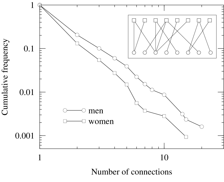
Figure 2: Distributions of the numbers of sexual contacts of men and women in the study of Liljeros et al. Liljeros01 . The histogram is cumulative, meaning that the vertical axis indicates the fraction of individuals studied who have greater than or equal to the number of contacts specified on the horizontal axis. Both distributions approximately follow power laws—straight lines on the logarithmic axes used here. Inset: the bipartite form of the modeled network of contacts.

V.1 Bipartite populations

Consider then a population of $M$ men and $N$ women, who have distributions $p_{j}$, $q_{k}$ of their numbers $j$ and $k$ of possibly disease-causing contacts with the opposite sex (connections in our nomenclature). In a recent study of 2810 respondents Liljeros et al. Liljeros01 recorded the numbers of sexual partners of men and women over the course of a year and found the distributions $p_{j}$, $q_{k}$ shown in Fig. 2. As the figure shows, the distributions appear to take a power-law form $p_{j}\sim j^{\alpha_{m}}$, $q_{k}\sim k^{\alpha_{f}}$, with exponents $\alpha_{m}$ and $\alpha_{f}$ that fall in the range $3.1$ to $3.3$ for both men and women . (The exponent for women seems to be a little higher than that for men, but the difference is smaller than the statistical error on the measurement.)

We will assume that the disease of interest is transmitted primarily by contacts between men and women (true only for some diseases in some communities HY84 ), so that, to a good approximation, the network of contacts is bipartite, as shown in the inset of Fig. 2. That is, there are two types of vertices representing men and women, and edges representing connections run only between vertices of unlike kinds. With each edge we associate two transmission rates, one of which represents the probability of disease transmission from male to female, and the other from female to male. These rates are drawn from appropriate distributions as before, as are the times for which men and women remain infective. Also as before, however, it is only the average integrated probability of transmission in each direction that matters for our percolation model, so that we have two transmissibilities $T_{mf}$ and $T_{fm}$ for the two directions .

We define two pairs of generating functions for the degree distributions of males and females:

$$f_{0}(x) = \sum_{j}p_{j}x^{j},\qquad f_{1}(x)=\frac{1}{\mu}f_{0}^{\prime}(x),$$ (48a)

$$g_{0}(x) = \sum_{k}q_{k}x^{k},\hskip 19.34787ptg_{1}(x)=\frac{1}{\nu}g_{0}^{\prime}(x),$$ (48b)

where $\mu$ and $\nu$ are the averages of the two degree distributions, and are related by

$${\mu\over M}={\nu\over N},$$ (49)

since the total numbers of edges ending at male and female vertices are necessarily the same. Using these functions we further define, as before

$$f_{0}(x;T) = f_{0}(1+(x-1)T),$$ (50a)

$$f_{1}(x;T) = f_{1}(1+(x-1)T),$$ (50b)

$$g_{0}(x;T) = g_{0}(1+(x-1)T),$$ (50c)

$$g_{1}(x;T) = g_{1}(1+(x-1)T).$$ (50d)

Now consider an outbreak that starts at a single individual, who for the moment we take to be male. From that male the disease will spread to some number of females, and from them to some other number of males, so that after those two steps a number of new males will have contracted the disease, whose distribution is generated by

$$F_{0}(x;T_{mf},T_{fm})=f_{0}(g_{1}(x;T_{fm});T_{mf}).$$ (51)

For a disease arriving at a male vertex along a randomly chosen edge we similarly have

$$F_{1}(x;T_{mf},T_{fm})=f_{1}(g_{1}(x;T_{fm});T_{mf}).$$ (52)

And one can define the corresponding generating functions $G_{0}$ and $G_{1}$ for the vertices representing the females.

Using these generating functions, we can now calculate generating functions $H_{0}$ and $H_{1}$ for the sizes of outbreaks of the disease in terms either of number of women or of number of men affected. The calculation proceeds exactly as in the unipartite case, and the resulting equations for $H_{0}$ and $H_{1}$ are identical to Eqs. (17) and (18). We can also calculate the average outbreak size and the size of an epidemic outbreak, if one is possible, from Eqs. (22), (25), and (26). The average outbreak size for males, for example, is

$$\left\langle s\right\rangle = 1+{F_{0}^{\prime}(1;T_{mf},T_{fm})\over 1-F_{1}^{\prime}(1;T_{fm},T_{mf})}$$ (53)

$$= 1+{T_{mf}T_{fm}f_{0}^{\prime}(1)g_{1}^{\prime}(1)\over 1-T_{mf}T_{fm}f_{1}^{\prime}(1)g_{1}^{\prime}(1)}.$$

The epidemic transition takes place when $F_{1}^{\prime}(1;T_{mf},T_{fm})=1$, or equivalently when

$$T_{mf}T_{fm}f_{1}^{\prime}(1)g_{1}^{\prime}(1)=1,$$ (54)

and hence the epidemic threshold takes the form of a hyperbola in $T_{mf}$–$T_{fm}$ space:

$$T_{mf}T_{fm}={1\over f_{1}^{\prime}(1)g_{1}^{\prime}(1)}={\mu\nu\over\sum_{j}j(j-1)p_{j}\sum_{k}k(k-1)p_{k}}.$$ (55)

Note that this expression is symmetric in the variables describing the properties of males and females. Although we derived it by considering the generating function for males $F_{1}$, we get the same threshold if we consider $G_{1}$ instead. Eq. (53) is not symmetric in this way, so that the typical numbers of males and females affected by an outbreak may be different. On the other hand Eq. (55) involves the transmissibilities $T_{mf}$ and $T_{fm}$ only in the form of their product, and hence the quantities of interest are a function only of a single variable $T_{mf}T_{fm}$.

The generalizations of Section IV, where we considered transmission probabilities that vary from one vertex to another, are possible also for the bipartite graph considered here. The derivations are straightforward and we leave them as an exercise for the reader.

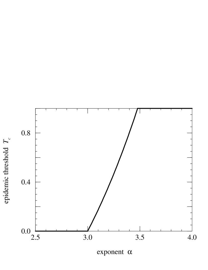
Figure 3: The critical transmissibility $T_{c}$ for the model of a sexually transmitted disease discussed in the text. $T_{c}$ is greater than zero and less than one only in the small range $3<\alpha<3.4788$ of the exponent $\alpha$.

V.2 Discussion

One important result that follows immediately from Eq. (55) is that if the degree distributions are truly power-law in form, then there exists an epidemic transition only for a small range of values of the exponent of the power law. Let us assume, as appears to be the case, that the exponents are roughly equal for men and women: $\alpha_{m}=\alpha_{f}=\alpha$. Then Eq. (55) tells us that the epidemic falls on the hyperbola $T_{mf}T_{fm}=T_{c}^{2}$, where

$$T_{c}={\zeta(\alpha-1)\over\zeta(\alpha-2)-\zeta(\alpha-1)},$$ (56)

where $\zeta(x)$ is the Riemann $\zeta$-function. The behavior of $T_{c}$ as a function of $\alpha$ is depicted in Fig. 3. As the figure shows, if $\alpha\leq 3$, $T_{c}=0$ and hence $T_{mf}T_{fm}=0$, which is only possible if at least one of the transmissibilities $T_{mf}$ and $T_{fm}$ is zero. As long as both are positive, we will always be in the epidemic regime, and this would clearly be bad news. No amount of precautionary measures to reduce the probability of transmission would ever eradicate the disease. (Lloyd and May LM01 have pointed out that a related result appears in the theory of fully mixed models, where a heterogeneous distribution of the infection parameter $\beta$ (see Eq. (1)) with a divergent coefficient of variation will result in the absence of an epidemic threshold. Pastor-Satorras and Vespignani PV01a have made similar predictions using mean-field-like solutions for SIRS-type endemic disease models on networks with power-law degree distributions and a similar result has also been reported for percolation models by Cohen et al. CEBH00 .) Conversely, if $\alpha>\alpha_{c}$, where $\alpha_{c}=3.4788\ldots$ is the solution of $\zeta(\alpha-2)=2\zeta(\alpha-1)$, we find that $T_{c}=1$ and hence $T_{mf}T_{fm}=1$, which is only possible if both $T_{mf}$ and $T_{fm}$ are 1. When either is less than 1 no epidemic will ever occur, which would be good news. Only in the small intermediate region $3<\alpha<3.4788$ does the model possess an epidemic transition. Interestingly, the real-world network measured by Liljeros et al. Liljeros01 appears to fall precisely in this region, with $\alpha\simeq 3.2$. If true, this would be both good and bad news. On the bad side, it means that epidemics can occur. But on the good side, it means that it is in theory possible to prevent an epidemic by reducing the probability of transmission, which is precisely what most health education campaigns attempt to do. The predicted critical value of the transmissibility is $T_{c}=0.363\ldots$ for $\alpha=3.2$. Epidemic behavior would cease were it possible to arrange for the transmissibility to fall below this value.

Some caveats are in order here. The error bars on the values of the exponent $\alpha$ are quite large (about $\pm 0.3$ Liljeros01 ). Thus, assuming that the conclusion of a power-law degree distribution is correct in the first place, it is still possible that $\alpha<3$, putting us in the regime where there is always epidemic behavior regardless of the value of the transmissibility. (The error bars are also large enough to put us in the regime $\alpha>\alpha_{c}$ in which there are no epidemics. Empirical evidence suggests that the real world is not in this regime however, since epidemics plainly do occur.)

It is also quite possible that the distribution is not a perfect power law. Although the measured distributions do appear to have power-law tails, it seems likely that these tails are cut off at some point. If this is the case, then there will always be an epidemic transition at finite $T$, regardless of the value of $\alpha$. Furthermore, if it were possible to reduce the number of partners that the most active members of the network have, so that the cutoff moves lower, then the epidemic threshold rises, making it easier to eradicate the disease. Interestingly, the fraction of individuals in the network whose degree need change in order to make a significant difference is quite small. At $\alpha=3$, for instance, a change in the value $\kappa$ of the cutoff from $\kappa=\infty$ to $\kappa=100$ affects only 1.3% of the population, but increases the epidemic threshold from $T_{c}=0$ to $T_{c}=0.52$. In other words, targeting preventive efforts at changing the behavior of the most active members of the network may be a much better way of limiting the spread of disease than targeting everyone. (This suggestion is certainly not new, but our models provide a quantitative basis for assessing its efficacy.)

Another application of the techniques presented here is described in Ref. ANMS02, . In that paper we model in detail the spread of walking pneumonia (Mycoplasma pneumoniae) in a closed setting (a hospital) for which network data are available from observation of an actual outbreak. In this example, our exact solutions agree well both with simulations and with data from the outbreak studied. Furthermore, examination of the analytic solution allows us to make specific suggestions about possible new control strategies for M. pneumoniae infections in settings of this type.

VI Conclusions

In this paper, we have shown that a large class of the so-called SIR models of epidemic disease can be solved exactly on networks of various kinds using a combination of mapping to percolation models and generating function methods. We have given solutions for simple unipartite graphs with arbitrary degree distributions and heterogeneous and possibly correlated infectiveness times and transmission probabilities. We have also given one example of a solution on a structured network—the spread of a sexually transmitted disease on a bipartite graph of men and women. Our methods provide analytic expressions for the sizes of both epidemic and non-epidemic outbreaks and for the position of the epidemic threshold, as well as network measures such as the mean degree of individuals affected in an epidemic.

Applications of the techniques described here are possible for networks specific to many settings, and hold promise for the better understanding of the role that network structure plays in the spread of disease.

- (1) N. T. J. Bailey, The Mathematical Theory of Infectious Diseases and its Applications. Hafner Press, New York (1975).
- (2) R. M. Anderson and R. M. May, Infectious Diseases of Humans. Oxford University Press, Oxford (1991).
- (3) H. W. Hethcote, Mathematics of infectious diseases. SIAM Review 42, 599–653 (2000).
- (4) S. H. Strogatz, Exploring complex networks. Nature 410, 268–276 (2001).
- (5) R. Albert and A.-L. Barabási, Statistical mechanics of complex networks. Rev. Mod. Phys. 74, 47–97 (2002).
- (6) D. J. Watts and S. H. Strogatz, Collective dynamics of ‘small-world’ networks. Nature 393, 440–442 (1998).
- (7) L. A. N. Amaral, A. Scala, M. Barthélémy, and H. E. Stanley, Classes of small-world networks. Proc. Natl. Acad. Sci. USA 97, 11149–11152 (2000).
- (8) F. Liljeros, C. R. Edling, L. A. N. Amaral, H. E. Stanley, and Y. Åberg, The web of human sexual contacts. Nature 411, 907–908 (2001).
- (9) M. Girvan and M. E. J. Newman, Community structure in social and biological networks. Proc. Natl. Acad. Sci. USA (in press).
- (10) J. Abello, A. Buchsbaum, and J. Westbrook, A functional approach to external graph algorithms. In Proceedings of the 6th European Symposium on Algorithms, Springer, Berlin (1998).
- (11) R. Albert, H. Jeong, and A.-L. Barabási, Diameter of the world-wide web. Nature 401, 130–131 (1999).
- (12) M. Faloutsos, P. Faloutsos, and C. Faloutsos, On power-law relationships of the internet topology. Computer Communications Review 29, 251–262 (1999).
- (13) A. Broder, R. Kumar, F. Maghoul, P. Raghavan, S. Rajagopalan, R. Stata, A. Tomkins, and J. Wiener, Graph structure in the web. Computer Networks 33, 309–320 (2000).
- (14) H. Jeong, B. Tombor, R. Albert, Z. N. Oltvai, and A.-L. Barabási, The large-scale organization of metabolic networks. Nature 407, 651–654 (2000).
- (15) H. Jeong, S. Mason, A.-L. Barabási, and Z. N. Oltvai, Lethality and centrality in protein networks. Nature 411, 41–42 (2001).
- (16) D. A. Fell and A. Wagner, The small world of metabolism. Nature Biotechnology 18, 1121–1122 (2000).
- (17) R. J. Williams and N. D. Martinez, Simple rules yield complex food webs. Nature 404, 180–183 (2000).
- (18) J. M. Montoya and R. V. Solé, Small world patterns in food webs. J. Theor. Bio. 214, 405–412 (2002).
- (19) C. Moore and M. E. J. Newman, Epidemics and percolation in small-world networks. Phys. Rev. E 61, 5678–5682 (2000).
- (20) M. Kuperman and G. Abramson, Small world effect in an epidemiological model. Phys. Rev. Lett. 86, 2909–2912 (2001).
- (21) R. Pastor-Satorras and A. Vespignani, Epidemic spreading in scale-free networks. Phys. Rev. Lett. 86, 3200–3203 (2001).
- (22) Y. Moreno, R. Pastor-Satorras, and A. Vespignani, Epidemic outbreaks in complex heterogeneous networks. Preprint cond-mat/0107267 (2001).
- (23) C. P. Warren, L. M. Sander, and I. Sokolov, Firewalls, disorder, and percolation in epidemics. Preprint cond-mat/0106450 (2001).
- (24) C. P. Warren, L. M. Sander, I. Sokolov, C. Simon, and J. Koopman, Percolation on disordered networks as a model for epidemics. Math. Biosci. (in press).
- (25) L. Sattenspiel and C. P. Simon, The spread and persistence of infectious diseases in structured populations. Math. Biosci. 90, 341–366 (1988).
- (26) I. M. Longini, A mathematical model for predicting the geographic spread of new infectious agents. Math. Biosci. 90, 367–383 (1988).
- (27) M. Kretzschmar and M. Morris, Measures of concurrency in networks and the spread of infectious disease. Math. Biosci. 133, 165–195 (1996).
- (28) F. Ball, D. Mollison, and G. Scalia-Tomba, Epidemics with two levels of mixing. Annals of Applied Probability 7, 46–89 (1997).
- (29) H. L. Frisch and J. M. Hammersley, Percolation processes and related topics. J. SIAM 11, 894–918 (1963).
- (30) P. Grassberger, On the critical behavior of the general epidemic process and dynamical percolation. Math. Biosci. 63, 157–172 (1983).
- (31) D. J. de S. Price, Networks of scientific papers. Science 149, 510–515 (1965).
- (32) A. L. Lloyd and R. M. May, How viruses spread among computers and people. Science 292, 1316–1317 (2001).
- (33) E. A. Bender and E. R. Canfield, The asymptotic number of labeled graphs with given degree sequences. Journal of Combinatorial Theory A 24, 296–307 (1978).
- (34) M. Molloy and B. Reed, A critical point for random graphs with a given degree sequence. Random Structures and Algorithms 6, 161–179 (1995).
- (35) M. Molloy and B. Reed, The size of the giant component of a random graph with a given degree sequence. Combinatorics, Probability and Computing 7, 295–305 (1998).
- (36) M. E. J. Newman, S. H. Strogatz, and D. J. Watts, Random graphs with arbitrary degree distributions and their applications. Phys. Rev. E 64, 026118 (2001).
- (37) M. E. J. Newman, D. J. Watts, and S. H. Strogatz, Random graph models of social networks. Proc. Natl. Acad. Sci. USA 99, 2566–2572 (2002).
- (38) R. Cohen, K. Erez, D. ben-Avraham, and S. Havlin, Resilience of the Internet to random breakdowns. Phys. Rev. Lett. 85, 4626–4628 (2000).
- (39) R. Cohen, K. Erez, D. ben-Avraham, and S. Havlin, Breakdown of the Internet under intentional attack. Phys. Rev. Lett. 86, 3682–3685 (2001).
- (40) D. S. Callaway, M. E. J. Newman, S. H. Strogatz, and D. J. Watts, Network robustness and fragility: Percolation on random graphs. Phys. Rev. Lett. 85, 5468–5471 (2000).
- (41) S. N. Dorogovtsev, J. F. F. Mendes, and A. N. Samukhin, Giant strongly connected component of directed networks. Phys. Rev. E 64, 025101 (2001).
- (42) L. A. Adamic, R. M. Lukose, A. R. Puniyani, and B. A. Huberman, Search in power-law networks. Phys. Rev. E 64, 046135 (2001).
- (43) H. Wilf, Generatingfunctionology. Academic Press, London, 2nd edition (1994).
- (44) C. Moore and M. E. J. Newman, Exact solution of site and bond percolation on small-world networks. Phys. Rev. E 62, 7059–7064 (2000).
- (45) M. E. J. Newman, The structure of scientific collaboration networks. Proc. Natl. Acad. Sci. USA 98, 404–409 (2001).
- (46) R. Pastor-Satorras and A. Vespignani, Immunization of complex networks. Phys. Rev. E 65, 036104 (2002).
- (47) T. B. Hyde, M. Gilbert, S. B. Schwartz, E. R. Zell, J. P. Watt, W. L. Thacker, D. F. Talkington, and R. E. Besser, Azithromycin prophylaxis during a hospital outbreak of Mycoplasma pneumoniae pneumonia. Journal of Infectious Diseases 183, 907–912 (2001).
- (48) H. W. Hethcote and J. A. Yorke, Gonorrhea Transmission Dynamics and Control. Springer, New York (1984).
- (49) L. W. Ancel, M. E. J. Newman, M. Martin, and S. Schrag, Applying network theory to epidemics: Modelling the spread and control of Mycoplasma pneumoniae. Working paper 01–12–078, Santa Fe Institute (2001).
- (50) S. Gupta, R. M. Anderson, and R. M. May, Networks of sexual contacts: Implications for the pattern of spread of HIV. AIDS 3, 807–817 (1989).
- (51) A. S. Klovdahl, J. J. Potterat, D. E. Woodhouse, J. B. Muth, S. Q. Muth, and W. W. Darrow, Social networks and infectious disease: The Colorado Springs study. Soc. Sci. Med. 38, 79–88 (1994).