Generating Generalized Distributions from Dynamical Simulation
Abstract
We present a general molecular-dynamics simulation scheme, based on the Nosé thermostat, for sampling according to arbitrary phase space distributions. We formulate numerical methods based on both Nosé-Hoover and Nosé-Poincaré thermostats for two specific classes of distributions; namely, those that are functions of the system Hamiltonian and those for which position and momentum are statistically independent. As an example, we propose a generalized variable temperature distribution that is designed to accelerate sampling in molecular systems.
I Introduction
Molecular-dynamics (MD) computer simulation is a widely used tool in biology, chemistry, physics and materials scienceFrenkel02 ; Allen87 . Much of the power in the technique lies in the ability to generate phase-space trajectories weighted according to a relevant statistical-mechanical distribution. In the first MD simulations, straightforward integration of the equations of motion for the system under study yielded energy conserving trajectories that, assuming ergodicity, generated microcanonical (constant ) equilibrium distributions of phase-space configurations. Later, to better mimic experimental conditions, a variety of MD techniques were developed that generate phase-space distributions according to other standard statistical-mechanical distributions, such as canonical ()Nose84a ; Hoover85 ; Bond99 , isothermal-isobaric ()Andersen80 ; Sturgeon00 , and grand-canonicalLynch97 . Recently, however, there has been growing interest in the simulation of systems with distributions that go beyond textbook statistical mechanical ensembles. For example, molecular-dynamics methods for the simulation of systems obeying Tsallis statisticsTsallis88 have been developed by Plastino and AnteneodoPlastino97 and Andriciaoaei and StraubAndricioaei97 . In this work we outline a general molecular-dynamics scheme, based on the Nosé thermostatNose84a ; Nose84b , to generate configurations according to an arbitrary phase-space distribution.
A primary motivation for the development of algorithms for the generation of non-standard distributions is the need for methods that accelerate the configurational sampling of systems. Many systems are not sufficiently ergodic on the time scale of standard molecular-dynamics simulations to ensure the convergence of statistical averages. This is especially true of macromolecules, biomolecules and amorphous materials. Over the past decade, a number of methods have been developed to enhance sampling in MD. Berne and StraubBerne97 have recently written an excellent review of new sampling methods. Central to these approaches has been the recognition that high activation barriers cause a bottleneck in phase space, rendering transitions between states unlikely. A common thread among many methods is the systematic deformation of the potential (or total) energy surface to accelerate barrier crossing, either by lowering the barriers or raising the potential valleys. From a statistical mechanical perspective, such energy modifications induce a corresponding modification in the phase-space distribution by enhancing the statistical weight of configurations in the vicinity of energy barriers. Explicit knowledge of the modified sampling distribution allows for statistical reweighting of the computed trajectories to achieve averages in the original ensemble.
The simplest method for enhancing sampling is to scale the full Hamiltonian by some factor less than unity. This is equivalent to performing the simulation at a higher temperature. If averages are desired at temperature , isothermal MD simulations can be carried out at some higher temperature , with averages at the original temperature computed by reweighting the probability of each configuration by a factor of . A significant disadvantage with such temperature boost approaches is that, unless the boost is sufficiently small, low energy configurations are not visited with a frequency large enough to obtain acceptable statistics. A related approach, Multicanonical MD, is based on a Monte Carlo technique of the same nameBerg91 and uses preliminary high temperature trajectories to construct a distribution that is nearly flat in the position coordinates, allowing nearly uniform sampling of coordinate space in subsequent simulations. Multicanonical MD has been demonstrated to accelerate conformational sampling in model polypeptidesNakajima97 and atomic clusters.
Another approach is Voter’s hyperdynamicsVoter96 ; Voter97 , which employs a “boost potential” to reduce the sampling probability in low energy regions, thereby accelerating barrier crossing due to diminished relative energetic cost. With boost potentials chosen to leave the potential energy in barrier regions unchanged, transition state theory arguments can be used to obtain good transition rate statistics. However, the low-energy sampling problem remains as in high temperature dynamics. Hyperdynamics has been used successfully in solid state systems, but the method is not generally applicable to liquids, where the presence of many saddle points hampers the identification of well-defined barrier regions.
Among recent methods of enhanced sampling, the approach of Straub and co-workersAndricioaei97 is of particular interest, with Monte Carlo and MD methods based on potential energy modifications that sample coordinates from alternative densities according to a formalism motivated by the non-extensive Tsallis entropyTsallis88 . The Tsallis-Straub approach is easy to implement, amounting to a simple modification of the interaction forces according to the gradient of an effective potential. Recently, a more direct application of Tsallis entropy to MD was suggested by Plastino and AnteneodoPlastino97 . Based on the idea of an effective Hamiltonian, these authors showed that canonical sampling with respect to the effective Hamiltonian is equivalent to Tsallis sampling. Significantly, this work considered only the Tsallis regime in which coordinate sampling is restricted to low energy regions.
In this paper we present a dynamical framework for sampling according to a general class of probability density functions, including but not limited to the Tsallis density. In order to introduce the idea of sampling from non-microcanonical distributions and to provide the necessary background for our generalized dynamics we discuss in Section II the extended Hamiltonian approach of NoséNose84a to canonical (constant temperature) sampling, as well as the Nosé-HooverHoover85 and Nosé-PoincaréBond99 approaches for implementing real-time formulations of Nosé dynamics. In Section III we introduce Generalized Distribution Dynamics (GDD) and discuss the technique for two special classes of systems: those for which the position and momentum distributions are separable and those for which the phase space distribution is a function of the full Hamiltonian, and show how the Nosé framework can be used to derive the equations of motion that produce trajectories that sample from generalized distributions. In section IV we present as an example the variable temperature distribution for accelerating the sampling of systems with high barriers. Numerical experiments on a double well potential using both the separable and full Hamiltonian GDD approaches are presented in section V.
II Sampling from a Canonical Distribution: the Nosé Thermostat
In traditional (NVE) MD simulation, the equations of motion corresponding to the system Hamiltonian, , are integrated to generate the trajectories. The trajectory is constrained to the constant energy surface, determined by the initial values of coordinates and momenta. States in phase space along solutions are said to be sampled from the microcanonical, or constant energy, distribution according to the probability density that is proportional to where is the Dirac delta function.
Due in part to a desire to bring simulation into accord with laboratory experiments that are typically conducted at some fixed temperature, methods have been developed for generating trajectories which sample from the canonical, or constant temperature, ensemble according to the probability density , which is proportional to where , being the temperature and the Boltzmann constant. In contrast to the microcanonical case, canonical sampling allows states at all energies, though higher energy states have lower probabilities depending on the value of temperature .
Although other methods exist, the most widely used techniques for generating canonically distributed trajectories in MD simulation are based on the extended Hamiltonian of NoséNose84a ; Nose84b :
| (1) |
where and are conjugate thermostat variables, is a fictional thermostat mass which determines the strength of thermal coupling to the system, (with being the number of degrees of freedom in the system) and is a virtual momentum related to the actual momentum of the system by Nose84a . The equations of motion generated by the Nosé Hamiltonian (Eq. 1) are
| (2) | |||||
| (3) | |||||
| (4) | |||||
| (5) |
The Nosé method regulates the temperature of the system through a dynamical time transformation given by , where is the Nosé (virtual) time and is real time. The remarkable property of Nosé dynamics is that microcanonical sampling of the extended phase space yields canonical sampling in the reduced phase space,, provided that the system is ergodic.
For practical calculations of averages such as velocity autocorrelation functions, it is convenient to work in a real time implementation of the Nosé thermostat. The most commonly used real-time modification is due to HooverHoover85 . Hoover recognized that one can generate a set of real-time equations of motion by making the following transformations to the Nosé equations of motion
-
1.
change of variables: .
-
2.
time transformation: ,
-
3.
change of variables: and .
The result is the following time-reversible system of equations, known as the Nosé-Hoover (NH) equationsHoover85 :
| (6) | |||||
| (7) | |||||
| (8) | |||||
| (9) |
where , the number of degrees of freedom in the system. These equations of motion are non-Hamiltonian in form since the coordinate transformations were not canonical; however, a conserved energy does exist given by
| (10) |
(Although the variable has been decoupled from the system, it is helpful to include it in the calculations so that can be monitored as an indicator of trajectory stability.)
Recently, Bond, Leimkuhler and LairdBond99 have developed an alternative real-time Nosé thermostat scheme, the Nosé-Poincaré method, which is Hamiltonian in form, allowing for the use of symplectic integration schemes (which have been shown to give superior stability in long time simulationSanz-Serna95 ). This is accomplished by performing a time transformation, not to the Nosé equations of motion as with Nosé-Hoover, but directly to the Hamiltonian using a Poincaré time transformation, as follows:
| (11) |
where is the initial value of . It can be easily verifiedBond99 that the phase space trajectory generated by is identical to that generated by except for a time transformation . The Nosé-Poincaré equations of motion are
| (12) | |||||
| (13) | |||||
| (14) | |||||
| (15) |
where
| (16) |
Note that, the exact solution to Nosé-Poincaré equations of motion generates trajectories that are identical to those generated by the Nosé-Hoover scheme, exactly solved. It is in the construction of approximate numerical methods that these two approaches differ.
Although we favor the Nosé-Poincaré method in all cases, the Nosé-Hoover formalism is more familiar within the simulation community. For this reason, in the current article, we present schemes based on both the Nosé-Hoover and Nosé-Poincaré approaches.
In certain systems, for example those with few particles or strong harmonic components, the ergodicity assumption basic to the Nosé approaches is not met. For these cases, the notion of Nosé-Hoover chains has been developedMartyna92 , in which the Hamiltonian is further extended with additional thermostat variables that are coupled to each other. It has been demonstrated that NH chains, with properly chosen thermostat masses, can induce the needed ergodicity so that NH dynamics provides a means of sampling from the canonical distribution. We discuss NH chains further in section V and in the Appendix.
III Generalized Distribution Dynamics
In this section we present a dynamical scheme for sampling points in phase space according to general function which satisfies the properties of a probability density function in the phase space variables :
In analogy to the procedure used by Plastino and AnteneodoPlastino97 to develop an MD method to generate the canonical Tsallis distribution, we relate the general density to the canonical density by way of an effective Hamiltonian as
which yields
| (17) |
It is clear that canonical sampling with respect to the effective Hamiltonian is equivalent to sampling according to the generalized probability density . To achieve canonical sampling with we write the Nosé Hamiltonian for Generalized Distribution Dynamics:
| (18) |
From the equations of motion generated from this Nosé Hamiltonian and after applying the transformations described in the previous section, we obtain the Nosé-Hoover GDD equations of motion:
| (19) | |||||
| (20) | |||||
| (21) | |||||
| (22) |
Similarly, the Nosé-Poincaré equations of motion for GDD are
| (23) | |||||
| (24) | |||||
| (25) | |||||
| (26) | |||||
These formulations disrupt the separability of variables present in the original NH and NP equations of motion [Eqs. (6)–(9) and (13–16), respectively]. A time reversible discretization of the GDD equations would involve the solution of nonlinear equations in and at every step. Iterative solution would require many evaluations of the potential energy and its gradient at each step, likely adding tremendously to the computational burden. We address this issue by considering two special classes of probability density u functions that maintain variable separability:
Case 1: GDD for Separable Distribution Functions
Consider separable probability distribution functions of the form
We can relate the separable density to the canonical density by way of effective kinetic and potential energies and as
leading to
| (27) |
Canonical sampling with respect to the effective Hamiltonian is equivalent to sampling according to the generalized probability density . Following the procedure outlined in the previous section, canonical sampling with can be achieved using the Nosé-Hoover GDD equations of
motion, which for a separable distribution function are obtained as:
| (28) | |||||
| (29) | |||||
| (30) | |||||
| (31) |
Generation of the Nosé-Poincaré equations of motion for this class of distributions follows similarly.
Note that these equations have a simple relationship with the NH equations (6)–(9). Any existing implementation of the NH (or NP) equations of motion can be easily modified for separable GDD by the replacement of by in equations (6), (9), and by in equation (7).
The most important applications for GDD for separable distributions are those in which only the coordinate distribution is altered through modification of the potential. Such potential-only modifications are at the heart of Voter dynamicsVoter97 and the Tsallis statistics based methods for accelerated sampling of Straub and AndricioaeiAndricioaei97 . For such systems is equal to its standard form and is given by eq. (27). Implementation of GDD for such systems is straightforward as any existing Nosé-Hoover (or Nosé-Poincaré) code could be used without modification (other than the use of a modified input potential surface).
Case 2: GDD for distributions that are functions of the Hamiltonian
Here we consider distributions that are formal functions of the scalar Hamiltonian: . Defining the effective Hamiltonian as
with associated Nosé Hamiltonian, the Nosé-Hoover GDD equations of motion for this case are
| (32) | |||||
| (33) | |||||
| (34) | |||||
| (35) |
We can arrive at the natural expression for the momenta by performing the time transformation :
| (36) | |||||
| (37) | |||||
| (38) | |||||
| (39) |
These equations have a suggestive form. The influence of the modified distribution is manifested solely in the thermostat variables. Deviation of from unity can be viewed as a time-dependent scaling of simulation temperature along with an inverse scaling of the thermostat mass .
It is possible to rewrite these equations yet again to achieve separation of the coordinates and momenta. Just as the quantity in (10) is constant along solutions of the NH equations, the GDD equations (36)–(39) conserve the related quantity
| (40) |
Making use of our assumption that and (and also ) is monotonic and hence one-to-one, we can solve (40):
and define a new function of and
| (41) |
so that the GDD equations become
| (42) | |||||
| (43) | |||||
| (44) | |||||
| (45) |
Equations (42)–(45) introduce coupling between the thermostat variables, but leave the coordinates and momenta separated, allowing for efficient discretization schemes. A similar trick can also be used to simplify the numerical calculations in the symplectic Nosé-Poincaré method. We discuss numerical methods in the appendix.
IV Example Application: A Variable Temperature Distribution
The methods of this paper are very general in the sense that dynamical simulations can be made to sample any smooth, invertible density function . In this section we propose a particular distribution function both for the purpose of demonstrating the methods of this paper and to outline a potentially useful method for accelerating sampling in systems with high barriers.
As mentioned earlier, one way to enhance the sampling of systems that are not ergodic on the time scale of standard simulation due to high barriers is to carry out the simulations at high temperature. The original distribution can the be recovered by reweighting the trajectory to compensate for the change in the distribution. However, for most situations the low energy configurations that have large weight in the original distribution are not sampled with sufficient frequency at high temperatures to yield adequate statistics after reweighting.
To address the low energy sampling problem with high temperatures, we propose a generalized distribution that has the effect of raising temperature only in high energy regions while leaving the low energy dynamics unaffected. To begin, we define the monotonic function , designed to smoothly switch between the identity function and a linear function of slope :
| (49) |
where control the size of the switching window and the shape of the switching function, and the polynomial coefficients of the switching function are given by
A graph of the function with , , , and is shown in the left view of Figure 2.
We now define a probability distribution as a function the Hamiltonian :
| (50) |
The same switching function can be used to generate a separable distribution with
| (51) |
in which the momentum distribution remains canonical. At (and ) both the Hamiltonian and potential versions of the variable temperature distribution reduce to the canonical distribution at temperature . For , the distributions give canonical sampling in low energy (total or potential, respectively) regions ( for some predetermined value ) of phase space at reference temperature while sampling high energy regions () at the higher temperature where . Note that approaches in the limit of large . This distribution modification has similarities with the Tsallis-based distributions used by Andricioaei and StraubAndricioaei97 and Plastino and AnteneodoPlastino97 in that the effective temperature is a monotonically increasing function of energy; however, in these cases the temperature (and thus the dynamics) is altered at all energies whereas in our present case the dynamics at low energies is unaltered.
V Numerical Experiments
To test our methods, we consider the double well potential
with minima at and barrier height .
We have performed a number of GDD simulations using the variable temperature distribution (50) in both its full Hamiltonian and potential forms. For all simulations, the reference temperature was . For such low dimensional systems it is necessary to use Nosé-Hoover chains to enhance the ergodicity of the dynamics — see the Appendix for discussion. In all simulations six thermostats were used. The switching window parameters in (49) were taken as , and (except when , then ). We report experiments with the variable temperature parameter =1.0, 0.9, 0.8, 0.7, 0.6, 0.5, 0.4, 0.3, 0.2. As decreases from unity, stability considerations dictate smaller timesteps. The timestep was for the modified potential energy calculations. For the full Hamiltonian approach, we use timestep .
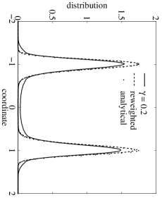
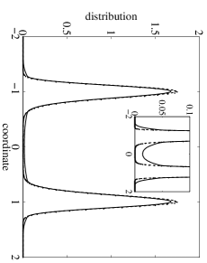
The left view of Figure 1 shows the distribution of coordinates for the full Hamiltonian calculations at . It can be seen by the good agreement with the theoretical distribution that the coordinates along the trajectory are sampled according to . Also shown is the reweighted distribution which recovers the canonical distribution. Note that at this temperature () standard NH chain dynamics fails to sample effectively. It must be pointed out that because the GDD equations for the full Hamiltonian case were derived with a time transformation in (41), it is necessary to include as a weighting function when computing averages using trajectories produced by equations (42)–(45). The right view of Figure 1 shows the distribution of coordinates for the modified potential calculations at . As for the results for the full Hamiltonian, it can be seen that the canonical coordinate distribution is also recovered by reweighting. Note that the unweighted coordinate distributions from the full Hamiltonian and modified potential formulations are not identical. In particular, the trajectory from the full Hamiltonian method spends slightly more time in high energy configurations.
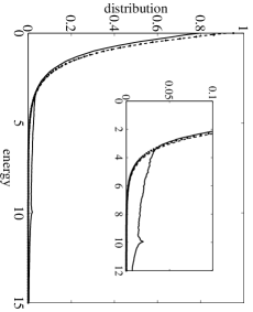
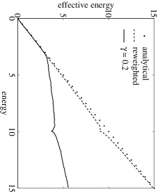
In Figure 2 we show the distribution of total energy along the computed full Hamiltonian trajectory for with , which can be seen to closely approximate the theoretical energy distribution for . Also shown is the function from equation (49), along with the computed values of calculated as the natural logarithm of the energy distribution from the trajectory.
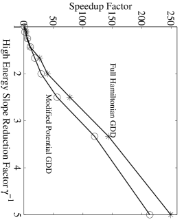
In Figure 3 we illustrate the success of the variable temperature density in hastening barrier crossings for the double well system. The figure shows waiting time plotted versus the temperature boost factor . It can be seen that both the full Hamiltonian and modified potential approaches yield dramatic reductions in waiting time between barrier crossings.
VI Conclusion
In this paper we have presented a general dynamical formalism, which we call Generalized Distribution Dynamics (GDD), that generates trajectories according to any of a broad class of probability distribution functions. In addition we show that the GDD scheme, which is based on the Nosé thermostatNose84a , can be easily implemented numerically for two classes of distribution functions: distributions that are functions of the full Hamiltonian and those that separate into a product of momentum and position distributions. In these two cases, the GDD scheme is equivalent to the dynamics of a system with a modified full Hamiltonian or effective potential energy surface, respectively. To implement GDD for these two classes, we outline specific numerical methods for both the Nosé-HooverHoover85 and Nosé-PoincaréBond99 real-time formulations of Nosé dynamics. As an example, we have introduced a specific form of a probability density function, the Variable Temperature Distribution, which has application in accelerating configurational sampling in systems with high energy barriers. To illustrate the numerical scheme and evaluate the method we performed numerical experiments using a one-dimensional bistable oscillator and demonstrate that the Variable Temperature Distribution is very effective for accelerated sampling of coordinates when used in the effective potential energy setting. We are currently applying this work to enhance the dynamical sampling of model polypeptides.
VII Acknowledgements
This work was undertaken during visits of EJB and BBL to the Centre for Mathematical Modelling at the University of Leicester, UK. Acknowledgment is made by EJB to the donors of The Petroleum Research Fund, administered by the ACS, for partial support of this research. BBL acknowledges the support of the National Science Foundation under grant CHE-9970903. BJL acknowledges the UK Engineering and Physical Sciences Research Council grant GR/R03259/01.
Appendix
A-1 Numerical Methods for Nosé-Hoover GDD for distributions that are functions of the Hamiltonian
The NH equations (6)–(9) can be discretized in a number of ways which generalize the basic Verlet approach. One such method is Martyna96 :
| (A-1) | |||||
| (A-2) | |||||
| (A-3) | |||||
| (A-4) | |||||
| (A-5) | |||||
| (A-6) | |||||
Equations (A-1) and (A-2) can be solved by computing the vector
and rewriting (A-2)
This scalar equation for can now be solved analytically or with an iterative solver. Using the computed , we can compute
The discretization scheme (A-1)–(A-6) can be generalized to the GDD equations (42)–(45):
| (A-7) | |||||
| (A-8) | |||||
| (A-9) | |||||
| (A-10) | |||||
| (A-11) | |||||
| (A-12) | |||||
| (A-13) | |||||
Two of the formulae are implicit. The procedure for is the same as for (A-8), while (A-11) may require the use of an iterative method, depending on the nature of the function . In the numerical results presented here, we use Newton-Raphson iteration with tolerance of in double precision.
The GDD scaling function introduced in equation (41) serves two interesting purposes. The resulting dynamical formalism retains the form of the NH equations, with coordinates and momenta coupled to a generalized thermostat (subject to a time transformation) via the thermostat variables and . From a practical point of view the introduction of allows for discretization schemes which are explicit in the coordinates and momenta, which is important for overall efficiency. Implementation of a timestepping scheme such as (A-7)–(A-13) requires repeated evaluation of the function , requiring the inversion of the function in (17) which defines the effective Hamiltonian of the generalized density. In general an analytic expression will not be available for . For the work described here, we have implemented the GDD scaling function using an algorithm which relies on the Newton-Raphson method for finding a zero of a scalar equation. For the variable temperature distribution based on (49), we evaluate by first evaluating from equation (41), then evaluating
and
With a good initial approximation (such as or the average ) the Newton-Raphson method above converges to the desired root with two or three iterations in our experience, subject to a convergence tolerance of in double precision calculations.
A-2 A symplectic numerical method for Nosé-Poincaré GDD for distributions that are functions of the Hamiltonian
Starting from the Nosé extended Hamiltonian applied to the effective Hamiltonian,
| (A-14) |
Assuming is one to one, we can invert to obtain, along the energy surface , the new Hamiltonian
| (A-15) |
The zero energy dynamics in this Hamiltonian correspond to dynamics. We next introduce a time-transformation of Poincaré type, resulting in
| (A-16) | |||||
It is natural to use a splitting method here, breaking the Hamiltonian into two parts according to the obvious additive decomposition and solving each term successively using an appropriate symplectic numerical method. Note that the splitting suggested here is different than that used recently by Nosé Nose00 in his variation of the Nosé-Poincaré method, but the basic technique is similar. Integration of the term
| (A-17) |
can be easily performed using the standard (and symplectic) Verlet method; note that during this fraction of the propagation timestep, will be constant. Formally, the integration of
| (A-18) |
can be done analytically. However, this is relatively painful. A simpler approach is to use an implicit method, such as the implicit midpoint method. For a general Hamiltonian , the midpoint method advances from step to step by solving
| (A-19) | |||||
| (A-20) |
where and is defined similarly. In the present case, this means solving a nonlinear system in at each timestep.
A-3 Nosé-Hoover chains
For systems that are small or contain stiff oscillatory components, lack of ergodicity may render the Nosé scheme ineffective. Chains of Nosé-Hoover thermostats have been shownMartyna92 to allow canonical sampling in these cases. For a chain of thermostat variables the equations of motion are
| (A-21) | |||||
| (A-22) | |||||
| (A-23) | |||||
| (A-24) | |||||
| (A-25) | |||||
| (A-27) | |||||
| (A-28) | |||||
| (A-29) | |||||
| (A-30) |
Along solutions of the Nosé-Hoover Chain (NHC) equations the conserved quantity is
| (A-31) | |||||
Discretization schemes for NH chains are discussed in References Jang97 and Martyna92 . Extension of Nosé-Poincaré to incorporate chains is somewhat delicate; this is work in progress by two of the authors.
References
- (1) D. Frenkel and B. Smit, Understanding Molecular Simulation, 2nd Ed., (Academic Press, New York, 2002).
- (2) M.A. Allen and D.J. Tildesley, Computer Simulation of Liquids, (Oxford Science Press, Oxford, 1987).
- (3) S. Nosé, Mol. Phys. 52, 255 (1984).
- (4) W.G. Hoover, Phys. Rev. A 31, 1695 (1985).
- (5) S.D. Bond, B.J. Leimkuhler, and B.B. Laird, J. Comp. Phys. 151, 114 (1999).
- (6) H.C. Andersen, J. Chem. Phys 72, 2384 (1980).
- (7) J.B. Sturgeon and B.B. Laird, J. Chem. Phys. 112, 3474 (2000).
- (8) G. Lynch and B.M. Pettit, J. Chem. Phys. 107, 8594 (1997).
- (9) C. Tsallis, J. Stat. Phys. 542, 479 (1988).
- (10) A.R. Plastino and C. Anteneodo, Ann. Phys. 255, 250 (1997).
- (11) I. Andricioaei and J.E. Straub, J. Chem. Phys. 107, 9117 (1997).
- (12) S. Nosé, J. Chem. Phys. 81, 511 (1984).
- (13) B.J. Berne and J.E. Straub, Curr. Opin. Struc. Biol 7, 181 (1997).
- (14) B.A. Berg and T. Neuhaus, Phys. Lett. B267, 249 (1991).
- (15) N. Nakajima, H. Nakamura, and K. Kidera, J. Chem. Phys. 101, 817 (1997).
- (16) A.F. Voter, J. Chem. Phys. 106, 465 (1996).
- (17) A.F. Voter, Phys. Rev Lett 78, 3908 (1997).
- (18) J.M. Sanz-Serna and M.P Calvo, Numerical Hamiltonian Problems, (Chapman and Hall, New York, 1995).
- (19) M.L. Klein G.J. Martyna and M. Tuckermann, J. Chem. Phys. 97, 2635 (1992).
- (20) Douglas J. Tobias Glenn J. Martyna, Mark E. Tuckerman and Michael L. Klein, Mol. Phys. 87, 1117 (1996).
- (21) S. Nosé, J. Phys. Soc. Japan 70, 75 (2000).
- (22) S. Jang and G.A. Madden, J. Chem. Phys. 107, 9514 (1997).