Volatility Fingerprints of Large Shocks:
Endogeneous Versus Exogeneous

Abstract

Finance is about how the continuous stream of news gets incorporated into prices. But not all news have the same impact. Can one distinguish the effects of the Sept. 11, 2001 attack or of the coup against Gorbachev on Aug., 19, 1991 from financial crashes such as Oct. 1987 as well as smaller volatility bursts? Using a parsimonious autoregressive process with long-range memory defined on the logarithm of the volatility, we predict strikingly different response functions of the price volatility to great external shocks compared to what we term endogeneous shocks, i.e., which result from the cooperative accumulation of many small shocks. These predictions are remarkably well-confirmed empirically on a hierarchy of volatility shocks. Our theory allows us to classify two classes of events (endogeneous and exogeneous) with specific signatures and characteristic precursors for the endogeneous class. It also explains the origin of endogeneous shocks as the coherent accumulations of tiny bad news, and thus unify all previous explanations of large crashes including Oct. 1987.

1 Introduction

A market crash occurring simultaneously on most of the stock markets of the world as witnessed in Oct. 1987 would amount to the quasi-instantaneous evaporation of trillions of dollars. Market crashes are the extreme end members of a hierarchy of market shocks, which shake stock markets repeatedly. Among recent events still fresh in memories are the Hong-Kong crash and the turmoil on US markets on oct. 1997, the Russian default in Aug. 1998 and the ensuing market turbulence in western stock markets and the collapse of the “new economy” bubble with the crash of the Nasdaq index in March 2000.

In each case, a lot of work has been carried out to unravel the origin(s) of the crash, so as to understand its causes and develop possible remedies. However, no clear cause can usually be singled out. A case in point is the Oct. 1987 crash, for which many explanations have been proposed but none has been widely accepted unambiguously. These proposed causes include computer trading, derivative securities, illiquidity, trade and budget deficits, over-inflated prices generated by speculative bubble during the earlier period, the auction system itself, the presence or absence of limits on price movements, regulated margin requirements, off-market and off-hours trading, the presence or absence of floor brokers, the extent of trading in the cash market versus the forward market, the identity of traders (i.e. institutions such as banks or specialized trading firms), the significance of transaction taxes, etc. More rigorous and systematic analyses on univariate associations and multiple regressions of these various factors conclude that it is not at all clear what caused the crash [Barro et al. (1989)]. The most precise statement, albeit somewhat self-referencial, is that the most statistically significant explanatory variable in the October crash can be ascribed to the normal response of each country’s stock market to a worldwide market motion [Barro et al. (1989)].

In view of the stalemate reached by the approaches attempting to find a proximal cause of a market shock, several researchers have looked for more fundamental origins and have proposed that a crash may be the climax of an endogeneous instability associated with the (rational or irrational) imitative behavior of agents (see for instance [Orléan (1989), Orléan (1995), Johansen and Sornette (1999), Shiller (2000)]). Are there qualifying signatures of such a mechanism? According to [Johansen and Sornette (1999), Sornette and Johansen (2001)] for which a crash is a stochastic event associated with the end of a bubble, the detection of such bubble would provide a fingerprint. A large literature has emerged on the empirical detectability of bubbles in financial data and in particular on rational expectation bubbles (see [Camerer (1989), Adam and Szafarz (1992)] for a survey). Unfortunately, the present evidence for speculative bubbles is fuzzy and unresolved at best, according to the standard economic and econometric literature. Other than the still controversial [Feigenbaum (2001)] suggestion that super-exponential price acceleration [Sornette and Andersen (2002)] and log-periodicity may qualify a speculative bubble [Johansen and Sornette (1999), Sornette and Johansen (2001)], there are no unambiguous signatures that would allow one to qualify a market shock or a crash as specifically endogeneous.

On the other end, standard economic theory holds that the complex trajectory of stock market prices is the faithful reflection of the continuous flow of news that are interpreted and digested by an army of analysts and traders [Cutler et al. (1989)]. Accordingly, large shocks should result from really bad surprises. It is a fact that exogeneous shocks exist, as epitomized by the recent events of Sept. 11, 2001 and the coup against Gorbachev on Aug., 19, 1991, and there is no doubt about the existence of utterly exogeneous bad news that move stock market prices and create strong bursts of volatility. However, some could argue that precursory fingerprints of these events were known to some elites, suggesting the possibility the action of these informed agents may have been reflected in part in stock markets prices. Even more difficult is the classification (endogeneous versus exogeneous) of the hierarchy of volatility bursts that continuously shake stock markets. While it is a common practice to associate the large market moves and strong bursts of volatility with external economic, political or natural events [White (1996)], there is not convincing evidence supporting it.

Here, we provide a clear and novel signature allowing us to distinguish between an endogeneous and an exogeneous origin to a volatility shock. Tests on the Oct. 1987 crash, on a hierarchy of volatility shocks and on a few of the obvious exogeneous shocks validate the concept. Our theoretical framework combines a rather novel but really powerful and parsimonious so-called multifractal random walk with conditional probability calculations.

2 Long-range memory and distinction between endogeneous and exogeneous shocks

While returns do not exhibit discernable correlations beyond a time scale of a few minutes in liquid arbitraged markets, the historical volatility (measured as the standard deviation of price returns or more generally as a positive power of the absolute value of centered price returns) exhibits a long-range dependence characterized by a power law decaying two-point correlation function [Ding et al. (1993), Ding and Granger (1996), Arneodo et al. (1998)] approximately following a $(t/T)^{-\nu}$ decay rate with an exponent $\nu\approx 0.2$. A variety of models have been proposed to account for these long-range correlations [Granger and Ding (1996), Baillie (1996), Müller et al. (1997), Muzy et al. (2000), Muzy et al. (2001), Müller et al. (1997)].

In addition, not only are returns clustered in bursts of volatility exhibiting long-range dependence, but they also exhibit the property of multifractal scale invariance (or multifractality), according to which moments $m_{q}\equiv\langle|r_{\tau}|^{q}\rangle$ of the returns at time scale $\tau$ are found to scale as $m_{q}\propto\tau^{\zeta_{q}}$, with the exponent $\zeta_{q}$ being a non-linear function of the moment order $q$ [Mandelbrot (1997), Muzy et al. (2000)].

To make quantitative predictions, we use a flexible and parsimonious model, the so-called multifractal random walk (MRW) (see Appendix A and [Muzy et al. (2000), Bacry et al. (2001)]), which unifies these two empirical observations by deriving naturally the multifractal scale invariance from the volatility long range dependence.

The long-range nature of the volatility correlation function can be seen as the direct consequence of a slow power law decay of the response function $K_{\Delta}(t)$ of the market volatility measured a time $t$ after the occurrence of an external perturbation of the volatility at scale $\Delta t$. We find that the distinct difference between exogeneous and endogeneous shocks is found in the way the volatility relaxes to its unconditional average value.

The prediction of the MRW model (see Appendix B for the technical derivation) is that the excess volatility ${\rm E}_{\rm exo}[\sigma^{2}(t)~{}|~{}{\omega}_{0}]-\overline{\sigma^{2}(t)}$, at scale $\Delta t$, due to an external shock of amplitude ${\omega}_{0}$ relaxes to zero according to the universal response

$${\rm E}_{\rm exo}[\sigma^{2}(t)~{}|~{}{\omega}_{0}]-\overline{\sigma^{2}(t)}\propto e^{2K_{0}t^{-1/2}}-1\approx\frac{2K_{0}}{\sqrt{t}}~{},$$ (1)

for not too small times, where $\overline{\sigma^{2}(t)}=\sigma^{2}{\Delta t}$ is the unconditional average volatility. This prediction is nothing but the response function $K_{\Delta t}(t)$ of the MRW model to a single piece of very bad news that is sufficient by itself to move the market significantly. This prediction is well-verified by the empirical data shown in figure 1.

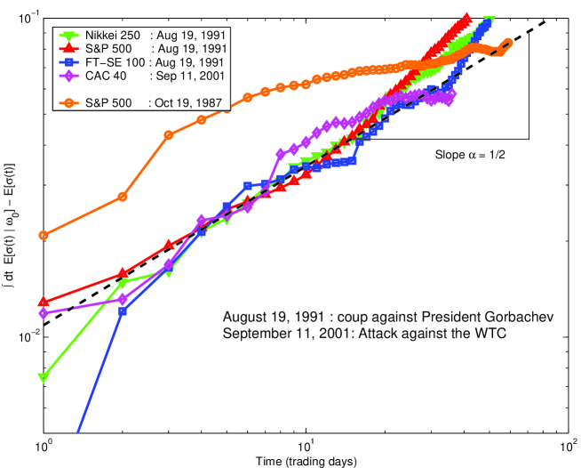
Figure 1: Cumulative excess volatility at scale $\Delta t=1$ day, that is, integral over time of ${\rm E}_{\rm exo}[\sigma^{2}(t)~{}|~{}{\omega}_{0}]-\overline{\sigma^{2}(t)}$, due to the volatility shock induced by the coup against President Gorbachev observed in three British, Japanese and USA indices and the shock induced by the attack of September 11, 2001 against the World Trade Center. The dashed line is the theoretical prediction obtained by integrating (1), which gives a $\propto\sqrt{t}$ time-dependence. The cumulative excess volatility following the crash of October 1987 is also shown with circles. Notice that the slope of the non-constant curve for the October 1987 crash is very different from the value $1/2$ expected and observed for exogeneous shocks. This crash and the resulting volatility relaxation can be interpreted as an endogeneous event.

On the other hand, an “endogeneous” shock is the result of the cumulative effect of many small bad news, each one looking relatively benign taken alone, but when taken all together collectively along the full path of news can add up coherently due to the long-range memory of the volatility dynamics to create a large “endogeneous” shock. This term “endogeneous” is thus not exactly adequate since prices and volatilities are always moved by external news. The difference is that an endogeneous shock in the present sense is the sum of the contribution of many “small” news adding up according to a specific most probable trajectory. It is this set of small bad news prior to the large shock that not only led to it but also continues to influence the dynamics of the volatility time series and creates an anomalously slow relaxation. Appendix C gives the derivation of the specific relaxation (21) associated with endogeneous shocks.

Figure 2: Measuring the conditional volatility response exponent $\alpha(s)$ for S&P 100 intradaily time series as a function of the endogeneous shock amplitude parameterized by $s$, defined by (19). (a) The original $5$ minute intradaily time series from 04/08/1997 to 12/24/2001. The $5$ minute de-seasonalized squared returns are aggregated in order to estimate the $40$ minutes and daily volatilities. (b) $40$ minute log-volatility covariance $C_{40}(\tau)$ as a function of the logarithm of the lag $\tau$. The MRW theoretical curve with $\lambda^{2}=0.018$ and $T=1$ year (dashed line) provides an excellent fit of the data up to lags of one month. (c) Conditional volatility response $\ln({\rm E}_{\rm endo}[\sigma^{2}(t)~{}|~{}s])$ as a function of $\ln(t)$ for three shocks with amplitudes given by $s=-1,0,1$. (d) Estimated exponent $\alpha(s)$ for ${\Delta t}=40$ minutes ($\bullet$) as a function of $s$. The solid line is the prediction corresponding to Eq. (22). The dashed line corresponds to the empirical MRW estimate obtained by averaging over 500 Monte-Carlo trials. It fits more accurately for negative $s$ (volatility lower than normal) due to the fact that the estimations of the variance by aggregation over smaller scales is very noisy for small variance values. The error bars give the 95 % confidence intervals estimated by Monte-Carlo trials of the MRW process. In the inset, $\alpha(s)$ is compared for ${\Delta t}=40$ minutes ($\bullet$) and ${\Delta t}=1$ day ($\times$).

Figure 2 reports empirical estimates of the conditional volatility relaxation after local maxima of the S&P100 intradaily series made of 5 minute close prices during the period from 04/08/1997 to 12/24/2001 (figure 1(a)). The original intraday squared returns have been preprocessed in order to remove the U-shaped volatility modulation associated with the intraday variations of market activity. Figure 2(b) shows that the MRW model provides a very good fit of the empirical volatility covariance in a range of time scales from $5$ minutes to one month. Fig. 2(c) plots in a double logarithmic representation, for the time scale ${\Delta t}=40$ minutes, the estimated conditional volatility responses for $s=1,0,-1$, where the endogeneous shocks are parameterized by $e^{2s}~{}\overline{\sigma^{2}(t)}$. A value $s>0$ (resp. $s<0$) corresponds to a positive bump (resp. negative dip) of the volatility above (resp. below) the average level $\overline{\sigma^{2}(t)}$. The straight lines are the predictions (Eqs. (24,22)) of the MRW model and qualify power law responses whose exponents $\alpha(s)$ are continuous function of the shock amplitude $s$. Figure 1(d) plots the conditional response exponent $\alpha(s)$ as a function of $s$ for the two time scales ${\Delta t}=40$ minutes and ${\Delta t}=$ 1 day (inset). For ${\Delta t}=40$ minutes, we observe that $\alpha$ varies between $-0.2$ for the largest positive shocks to $+0.2$ for the largest negative shocks, in excellent agreement with MRW estimates (dashed line) and, for $\alpha\geq 0$, with Eq. (22) obtained without any adjustable parameters. The error bars represent the 95 % confidence intervals estimated using 500 trials of synthetic MRW with the same parameters as observed for the S&P 100 series. By comparing $\alpha(s)$ for different ${\Delta t}$ (inset), we can see the the MRW model is thus able to recover not only the $s$-dependence of the exponent $\alpha(s)$ of the conditional response function to endogeneous shocks but also its time scale ${\Delta t}$ variations: this exponent increases as one goes from fine to coarse scales. Similar results are obtained for other intradaily time series (Nasdaq, FX-rates, etc.). We also obtain the same results for 17 years of daily return times series of various indices (French, German, canada, Japan, etc.).

In summary, the most remarkable result is the qualitatively different functional dependence of the response (1) to an exogeneous compared to the response (24,22) to an endogeneous shock. The former gives a decay of the burst of volatility $\propto 1/t^{1/2}$ compared to $1/t^{\alpha(s)}$ for endogeneous shocks with amplitude $e^{2s}~{}\overline{\sigma^{2}(t)}$, with an exponent $\alpha(s)$ being a linear function of $s$.

3 Discussion

What is the source of endogeneous shocks characterized by the response function (21)? Appendix D and equation (29) predict that the expected path of the continuous information flow prior to the endogeneous shock grows proportionally to the response function $K(t_{c}-t)$ measured in backward time to the shock occuring at $t_{c}$. In other words, conditioned on the observation of a large endogeneous shock, there is specific set of trajectories of the news flow that led to it. This specific flow has an expectation given by (29). This result allows us to understand the distinctive features of an endogeneous shock compared to an external shock. The later is a single piece of very bad news that is sufficient by itself to move the market significantly according to (1). In contrast, an “endogeneous” shock is the result of the cumulative effect of many small bad news, each one looking relatively benign taken alone, but when taken all together collectively along the full path of news can add up coherently due to the long-range memory of the log-volatility dynamics to create a large “endogeneous” shock. This term “endogeneous” is thus not exactly adequate since prices and volatilities are always moved by external news. The difference is that an endogeneous shock in the present sense is the sum of the contribution of many “small” news adding up according to a specific most probable trajectory. It is this set of small bad news prior to the large shock that not only led to it but also continues to influence the dynamics of the volatility time series and creates the anomalously slow relaxation (21).

In this respect, this result allows us to rationalize and unify the many explanations proposed to account for the Oct. 1987 crash: according to the present theory, each of the explanations is insufficient to explain the crash; however, our theory suggests that it is the cumulative effect of many such effects that led to the crash. In a sense, the different commentators and analysts were all right in attributing the origin of the Oct. 1987 crash to many different factors but they missed the main point that the crash was the extreme response of the system to the accumulation of many tiny bad news contributions. To test this idea, we note that the decay of the volatility response after the Oct. 1987 crash has been described by a power law $1/t^{0.3}$ [Lillo and Mantegna (2001)], which is in line with the prediction of our MRW theory with equation (22) for such a large shock (see also figure 2 panel d). This value of the exponent is still significantly smaller than $0.5$. Figure 1 demonstrates further the difference between the relaxation of the volatility after this event shown with circle and those following the exogenous coup against Gorbachev and the September 11 attack. There is clearly a strong constrast which qualifies the Oct. 1987 crash as endogeneous, in the sense of our theory of “conditional response.” This provides an independent confirmation of the concept advanced before in [Johansen and Sornette (1999), Sornette and Johansen (2001)].

It is also interesting to compare the prediction (21) with those obtained with a linear autoregressive model of the type (5), in which ${\omega}(t)$ is replaced by $\sigma(t)$. FIGARCH models fall in this general class. It is easy to show in this case that this linear (in volatility) model predicts the same exponent for the response of the volatility to endogeneous shocks, independently of their magnitude. This prediction is in stark constrast with the prediction (21) of the log-volatility MRW model. The later model is thus strongly validated by our empirical tests.

Appendix A: The Multifractal Randow Walk (MRW) model

The multifractal random walk model is the continuous time limit of a stochastic volatility model where log-volatility correlations decay logarithmically. It possesses a nice “stability” property related to its scale invariance property: For each time scale ${\Delta t}\leq T$, the returns at scale ${\Delta t}$, $r_{{\Delta t}}(t)\equiv\ln[p(t)/p(t-{\Delta t})]$, can be described as a stochastic volatility model:

$$r_{{\Delta t}}(t)=\epsilon(t)\cdot\sigma_{{\Delta t}}(t)=\epsilon(t)\cdot e^{{\omega}_{{\Delta t}}(t)}~{},$$ (2)

where $\epsilon(t)$ is a standardized Gaussian white noise independent of ${\omega}_{{\Delta t}}(t)$ and ${\omega}_{{\Delta t}}(t)$ is a nearly Gaussian process with mean and covariance:

$$\mu_{{\Delta t}} = {1\over 2}\ln(\sigma^{2}{\Delta t})-C_{\Delta t}(0)$$ (3)

$$C_{\Delta t}(\tau) = {\rm Cov}[{\omega}_{{\Delta t}}(t),{\omega}_{{\Delta t}}(t+\tau)]=\lambda^{2}\ln\left(\frac{T}{|\tau|+e^{-3/2}{\Delta t}}\right)~{}.$$ (4)

$\sigma^{2}{\Delta t}$ is the return variance at scale ${\Delta t}$ and $T$ represents an “integral” (correlation) time scale. Such logarithmic decay of log-volatility covariance at different time scales has been demonstrated empirically in [Arneodo et al. (1998), Muzy et al. (2000)]. Typical values for $T$ and $\lambda^{2}$ are respectively $1$ year and $0.02$. According to the MRW model, the volatility correlation exponent $\nu$ is related to $\lambda^{2}$ by $\nu=4\lambda^{2}$.

The MRW model can be expressed in a more familiar form, in which the log-volatility $\omega_{\Delta t}(t)$ obeys an auto-regressive equation whose solution reads

$$\omega_{\Delta t}(t)=\mu_{\Delta t}+\int_{-\infty}^{t}d\tau~{}\eta(\tau)~{}K_{\Delta t}(t-\tau)~{},$$ (5)

where $\eta(t)$ denotes a standardized Gaussian white noise and the memory kernel $K_{\Delta t}(\cdot)$ is a causal function, ensuring that the system is not anticipative. The process $\eta(t)$ can be seen as the information flow. Thus ${\omega}(t)$ represents the response of the market to incoming information up to the date $t$. At time $t$, the distribution of ${\omega}_{\Delta t}(t)$ is Gaussian with mean $\mu_{\Delta t}$ and variance $V_{\Delta t}=\int_{0}^{\infty}d\tau~{}K^{2}_{\Delta t}(\tau)=\lambda^{2}\ln\left(\frac{Te^{3/2}}{\Delta t}\right)$. Its covariance, which entirely specifies the random process, is given by

$$C_{\Delta t}(\tau)=\int_{0}^{\infty}dt~{}K_{\Delta t}(t)K_{\Delta t}(t+|\tau|)~{}.$$ (6)

Performing a Fourier tranform, we obtain $\hat{K}_{\Delta t}(f)^{2}=\hat{C}_{\Delta t}(f)=2\lambda^{2}~{}f^{-1}\left[\int_{0}^{Tf}{\sin(t)\over t}dt+O\left(f{\Delta t}\ln(f{\Delta t})\right)\right]$, which shows that for $\tau$ small enough

$$K_{\Delta t}(\tau)\sim K_{0}\sqrt{\frac{\lambda^{2}T}{\tau}}~{}~{}~{}~{}~{}\mbox{for}~{}~{}{\Delta t}<<\tau<<T~{}.$$ (7)

This slow power law decay (7) of the memory kernel in (5) ensures the long-range dependence and multifractality of the stochastic volatility process (2). Note that equation (5) for the log-volatility ${\omega}_{\Delta t}(t)$ takes a form similar to but simpler than the ARFIMA models usually defined on the (linear) volatility $\sigma$ [Baillie (1996)].

Appendix B: Linear response to an external shock

Let us assume that new major piece of information $\eta(t)={\omega}_{0}~{}\delta(t)$ impinges on the market at some time (taken without loss of generality to be $t=0$, since the system is stationary). ${\omega}_{0}$ is the amplitude of the external shock. Then, using the formalism of Appendix A, the response of the log-volatility ${\omega}(t)$, $t>0$ to this shock is

$${\omega}(t) = \mu+\int_{-\infty}^{t}d\tau~{}[{\omega}_{0}\cdot\delta(\tau)+\eta(\tau)]~{}K(t-\tau)$$ (8)

$$= \mu+{\omega}_{0}~{}K(t)+\int_{-\infty}^{t}d\tau~{}\eta(\tau)~{}K(t-\tau)~{}.$$ (9)

where, for notation convenience, we have omitted the reference to the scale ${\Delta t}$. The expected volatility conditional on this incoming major information is thus

$${\rm E}_{\rm exo}[\sigma^{2}(t)~{}|~{}{\omega}_{0}] = {\rm E}_{\rm exo}\left[e^{2w(t)}~{}|~{}{\omega}_{0}\right]=e^{2{\omega}_{0}~{}K(t)}~{}{\rm E}\left[e^{2\int_{-\infty}^{t}d\tau~{}\eta(\tau)~{}K(t-\tau)}\right]~{}=\overline{\sigma^{2}(t)}e^{2{\omega}_{0}~{}K(t)}$$ (10)

$$\simeq \overline{\sigma^{2}(t)}e^{2K_{0}\sqrt{\lambda^{2}T\over t}}\;~{}\mbox{for}~{}\;{\Delta t}<<t<<T.$$ (11)

For time $t$ large enough, the volatility relaxes to its unconditional average value $\overline{\sigma^{2}(t)}=\sigma^{2}{\Delta t}$, so that the excess volatility ${\rm E}_{\rm exo}[\sigma^{2}(t)~{}|~{}{\omega}_{0}]-\overline{\sigma^{2}(t)}$ due to the external shock decays to zero as

$${\rm E}_{\rm exo}[\sigma^{2}(t)~{}|~{}{\omega}_{0}]-\overline{\sigma^{2}(t)}\propto\frac{1}{\sqrt{t}}~{}.$$ (12)

This universal response of the volatility to an external shock (i.e., independent of the amplitude ${\omega}_{0}$ of the shock) is governed by the time-dependence (7) of the memory kernel $K(t)$. Note also that the exponent $1/2$ of this power law decay does not depend on the specific functional form choosen for the volatility. Indeed, we could have choosen to define the volatily by the expectation of any power of the absolute returns, the exponent $1/2$ of the power law would have remain the same.

Appendix C: “Conditional response” to an endogeneous shock

Let us consider the natural evolution of the system, without any large external shock, which nevertheless exhibits a large volatility burst ${\omega}(t=0)={\omega}_{0}$ at $t=0$. From the definition (2) with (5) and (6), it is clear that a large “endogeneous” shock requires a special set of realization of the “small news” $\{\eta(t)\}$. To quantifies the response in such case, we can evaluate ${\rm E}_{\rm endo}[\sigma^{2}(t)~{}|~{}{\omega}_{0}]={\rm E}_{\rm endo}[e^{2{\omega}(t)}~{}|~{}{\omega}_{0}]$. Since ${\omega}(t)$ is a Gaussian process, the new process ${\omega}(t)$ conditional on ${\omega}_{0}$ remains Gaussian, so that

$${\rm E}_{\rm endo}[\sigma^{2}(t)~{}|~{}{\omega}_{0}] = {\rm E}_{\rm endo}[e^{2{\omega}(t)}~{}|~{}{\omega}_{0}]$$ (13)

$$= \exp\left(2{\rm E}[w(t)~{}|~{}{\omega}_{0}]+2{\rm Var}[{\omega}(t)~{}|~{}{\omega}_{0}]\right).$$ (14)

Due to the still Gaussian nature of the condition log-volatility ${\omega}(t)$, we easily obtain using (3) and (4),

$${\rm E}_{\rm endo}[{\omega}(t)~{}|~{}{\omega}_{0}] = {\rm E}[{\omega}(t)]+\frac{{\rm Cov}[{\omega}(t),{\omega}_{0}]}{{\rm Var}[{\omega}_{0}]}\cdot\left({\omega}_{0}-{\rm E}[{\omega}_{0}]\right),$$ (15)

$$= ({\omega}_{0}-\mu)\cdot\frac{C(t)}{C(0)}+\mu~{},$$ (16)

and

$${\rm Var}_{\rm endo}[{\omega}(t)~{}|~{}{\omega}_{0}] = {\rm Var}[{\omega}(t)]-\frac{{\rm Cov}[{\omega}(t),{\omega}_{0}]^{2}}{{\rm Var}[{\omega}_{0}]},$$ (17)

$$= C(0)\left(1-\frac{C^{2}(t)}{C^{2}(0)}\right)~{}.$$ (18)

Let us set:

$$e^{2{\omega}_{0}}=e^{2s}\overline{\sigma^{2}(t)}\Rightarrow{\omega}_{0}-\mu=s+C(0)$$ (19)

By subsitution in (14), we obtain thanks to (3) and (4),

$${\rm E}_{\rm endo}[\sigma^{2}(t)~{}|~{}{\omega}_{0}] = \overline{\sigma^{2}(t)}\exp\left[2({\omega}_{0}-\mu)\cdot\frac{C(t)}{C(0)}-2\frac{C^{2}(t)}{C(0)}\right],$$ (20)

$$= \overline{\sigma^{2}(t)}\left({T\over t}\right)^{\alpha(s)+\beta(t)}$$ (21)

where

$$\alpha(s) = {2s\over\ln({Te^{3/2}\over{\Delta t}})}~{},$$ (22)

$$\beta(t) = 2\lambda^{2}{\ln(t/{\Delta t})\over\ln(Te^{3/2}/{\Delta t})}~{}.$$ (23)

Within the range ${\Delta t}<t<<{\Delta t}e^{|s|\over\lambda^{2}}$, $\beta(t)<<\alpha(s)$ and Eq. (21) leads to a power-law behavior:

$${\rm E}_{\rm endo}[\sigma^{2}(t)~{}|~{}{\omega}_{0}]\sim t^{-\alpha(s)}$$ (24)

Notice that $|s|\lambda^{-2}$ provides directly the logarithmic scaling range over which the power-law can be observed. Since $\lambda^{-2}\sim 20$, this range can quickly extend over the whole time domain $[\ln({\Delta t}),\ln(T)]$.

Along the same line, we can also compute the conditional variance ${\rm Var}\left[\sigma^{2}(t)~{}|~{}{\omega}_{0}\right]$. After a little algebra, we get:

$${\rm Var}_{\rm endo}\left[\sigma^{2}(t)~{}|~{}{\omega}_{0}\right]=\overline{\sigma^{2}(t)}^{2}\left({T\over t}\right)^{2\alpha(s)+2\beta(t)}\left(({Te^{3/2}\over{\Delta t}})^{4\lambda^{2}}({T\over t})^{-2\beta^{\prime}(t)}-1\right)$$ (25)

where

$$\beta^{\prime}(t)=2\lambda^{2}{\ln(T/t)\over\ln(Te^{3/2}/{\Delta t})}$$ (26)

It is thus easy to obtain the estimate:

$$\sqrt{{\rm Var}_{\rm endo}\left[\sigma^{2}(t)~{}|~{}{\omega}_{0}\right]}\leq{\rm E}_{\rm endo}[\sigma^{2}(t)~{}|~{}{\omega}_{0}]\left(({T\over{\Delta t}})^{2\beta(t)}-1\right)^{1/2}\lesssim\sqrt{6\lambda^{2}\ln(te^{3/2}/\Delta t)}~{}~{}{\rm E}_{\rm endo}[\sigma^{2}(t)~{}|~{}{\omega}_{0}]$$ (27)

We thus conclude, that, for $s$ large enough (i.e., $\alpha(s)$ large enough):

$${{\rm E}_{\rm endo}[\sigma^{2}(t)~{}|~{}{\omega}_{0}]-\overline{\sigma^{2}(t)}\over\sqrt{{\rm Var}_{\rm endo}\left[\sigma^{2}(t)~{}|~{}{\omega}_{0}\right]}}\gtrsim{1\over\sqrt{6\lambda^{2}\ln(te^{3/2}/\Delta t)}}$$ (28)

Over the first decade ${\Delta t}\leq t\leq 10{\Delta t}$, the deviation of the conditional mean volatility from the unconditional volatility $\overline{\sigma^{2}(t)}$ is greater than the conditional variance, which ensures the existence of a strong deterministic component of the conditional response above the stochastic components.

Expressions (24,22) are our two main predictions. These equations predict that the conditional response function ${\rm E}_{\rm endo}[\sigma^{2}(t)~{}|~{}{\omega}_{0}]$ of the volatility decays as a power law $\sim 1/t^{\alpha}$ of the time since the endogeneous shock, with an exponent $\alpha\approx\left(2{\omega}_{0}-\ln(\overline{\sigma^{2}(t)})\right)\frac{\lambda^{2}}{C(0)}$ which depends linearly upon the amplitude ${\omega}_{0}$ of the shock. Note in particular, that $\alpha$ changes sign: it is positive for $w_{0}>{1\over 2}\ln(\overline{\sigma^{2}(t)})$ and negative otherwise.

Appendix D: Determination of the sources of endogeneous shocks

What is the source of endogeneous shocks characterized by the response function (21)? To answer, let us consider the process $W(t)\equiv\int_{-\infty}^{t}d\tau~{}\eta(\tau)$, where $\eta(t)$ is a standardized Gaussian white noise which captures the information flow impacting on the volatility, as defined in (5). Extending the property (16), we find that

$${\rm E}_{\rm endo}[W(t)~{}|~{}{\omega}_{0}]=\frac{{\rm Cov}[W(t),{\omega}_{0}]}{{\rm Var}[{\omega}_{0}]}\cdot\left({\omega}_{0}-{\rm E}[{\omega}_{0}]\right)\propto\left({\omega}_{0}-{\rm E}[{\omega}_{0}]\right)\int_{-\infty}^{t}d\tau~{}K(-\tau)~{}.$$ (29)

Expression (29) predicts that the expected path of the continuous information flow prior to the endogeneous shock (i.e., for $t<0$) grows like $\Delta W(t)=\eta(t)\Delta t\sim K(-t)\Delta t\sim\Delta t/\sqrt{-t}$ for $t<0$ upon the approach to the time $t=0$ of the large endogeneous shock. In other words, conditioned on the observation of a large endogeneous shock, there is specific set of trajectories of the news flow $\eta(t)$ that led to it. These conditional news flows have an expectation given by (29).

References

- [Adam and Szafarz (1992)] Adam, M.C. and A. Szafarz, 1992, Speculative Bubbles and Financial Markets, Oxford Economic Papers 44, 626-640.
- [Arneodo et al. (1998)] Arneodo, A., J.F. Muzy and D. Sornette, 1998, Direct causal cascade in the stock market, The European physical Journal B 2, 277-282.
- [Bacry et al. (2001)] Bacry, E., J. Delour and J.F. Muzy, 2001, Multifractal ranom walk, Physical Review E 64, 026103.
- [Baillie (1996)] Baillie, R.T., 1996, Long memory processes and fractional integration in econometrics, Journal of Econometrics 73, 5-59.
- [Barro et al. (1989)] Barro, R.J., E.F. Fama, D.R. Fischel, A.H. Meltzer, R. Roll and L.G. Telser, 1989, Black monday and the future of financial markets, edited by R.W. Kamphuis, Jr., R.C. Kormendi and J.W.H. Watson (Mid American Institute for Public Policy Research, Inc. and Dow Jones-Irwin, Inc.).
- [Camerer (1989)] Camerer, C., 1989, Bubbles and Fads in Asset Prices, Journal of Economic Surveys 3, 3-41.
- [Cutler et al. (1989)] Cutler, D., J. Poterba and L. Summers, What Moves Stock Prices? 1989, Journal of Portfolio Management, Spring, 4-12.
- [Ding et al. (1993)] Ding, Z., Granger, C.W.J. and Engle, R., 1993, A long memory property of stock returns and a new model, Journal of Empirical Finance 1, 83-106.
- [Ding and Granger (1996)] Ding, Z., Granger, C.W.J., 1996, Modeling volatility persistence of speculative returns: A new approach, Journal of Econometrics 73, 185-215.
- [Feigenbaum (2001)] Feigenbaum, J.A., 2001, A statistical analysis of log-periodic precursors to financial crashes, Quantitative Finance 1(3), 346-360.
- [Granger and Ding (1996)] Granger, C.W.J. and Ding, Z., 1996, Varieties of long memory models, Journal of Econometrics 73, 61-77.
- [Johansen and Sornette (1999)] Johansen, A. and Sornette, 1999, Critical Crashes, Risk 12 (1), 91-94.
- [Lillo and Mantegna (2001)] Lillo, F. and R.N. Mantegna, Power-law relaxation in a complex system: the fluctuation decay after a financial market crash, preprint cond-mat/0111257
- [Mandelbrot (1997)] Mandelbrot, B.B., 1997, Fractals and scaling in finance : discontinuity, concentration, risk : selecta volume E, New York : Springer.
- [Müller et al. (1997)] Müller, U.A., M.M. Dacorogna, R. Dav , R.B. Olsen, O.V. Pictet and J.E. von Weizs”cker, 1997, Volatilities of Different Time Resolutions - Analyzing the Dynamics of Market Components, Journal of Empirical Finance 4, No. 2-3, 213-240.
- [Muzy et al. (2000)] Muzy, J.F., J. Delour and E. Bacry, 2000, Modelling fluctuations of financial time series: from cascade process to stochastic volatility model, The European physical Journal B 17, 537-548.
- [Muzy et al. (2001)] Muzy, J.-F., D. Sornette, J. Delour and A. Arneodo, 2001, Multifractal returns and Hierarchical Portfolio Theory, Quantitative Finance 1 (1), 131-148.
- [Orléan (1989)] Orléan, A., 1989, Mimetic contagion and speculative bubbles, Theory and Decision 27, 63-92.
- [Orléan (1995)] Orléan, A., 1995, Bayesian interactions and collective dynamics of opinion: Heard behavior and mimetic contagion, journal of Economic Behavior & Organization 28, 257-274.
- [Kim et al. (1998)] Kim, S., N. Shepard, and S. Chib , 1998, Stochastic volatility: Likelyhood inference and comparison with ARCH models, Review of Economic Studies 65, 361-393.
- [Shiller (2000)] Shiller, R.J., 2000, Irrational exuberance (Princeton University Press, Princeton, NJ).
- [Sornette and Johansen (2001)] Sornette, D. and A. Johansen, 2001, Significance of log-periodic precursors to financial crashes, Quantitative Finance 1 (4), 452-471.
- [Sornette and Andersen (2002)] Sornette, D. and J.V. Andersen, 2002, A Nonlinear Super-Exponential Rational Model of Speculative Financial Bubbles, Int. J. Mod. Phys. C 13 (2), 171-188.
- [White (1996)] White E.N., 1996, Stock market crashes and speculative manias. In The international library of macroeconomic and financial history, 13 (An Elgar Reference Collection, Cheltenham, UK; Brookfield, US).