Journal of Physics: Condensed Matter 14 (2002) 21
Stripe formation in high-$T_{c}$ superconductors

Abstract

The non-uniform ground state of the two-dimensional three-band Hubbard model for the oxide high-$T_{c}$ superconductors is investigated using a variational Mont Carlo method. We examine the effect produced by holes doped into the antiferromagnetic (AF) background in the underdoped region. It is shown that the AF state with spin modulations and stripes is stabilized due to holes travelling in the CuO plane. The structures of modulated AF spins are dependent upon the parameters used in the model. The effect of boundary conditions is reduced for large systems. We show that there is a region where incommensurability is proportional to the hole density. Our results give a consistent description of stripes observed by the neutron scattering experiments based on the three-band model for the CuO plane.

I Introduction

A mechanism of superconductivity of high-$T_{c}$ cuprates is not still clarified after the intensive efforts over a decade. An origin of the anomalous metallic properties in the underdoped region has also been investigated by many physicists as a challenging problem. In order to solve the mysteries of high-$T_{c}$ cuprates, it is important to examine the ground state of the two-dimensional CuO₂ planes which are usually contained in the crystal structures of high-$T_{c}$ oxide superconductors.^? A basic model for the CuO₂ plane is the two-dimensional three-band Hubbard model with $d$ and $p$ orbitals, which is expected to contain essential features of high-$T_{c}$ cuprates.^?? The undoped oxide compounds exhibit a rich structure of antiferromagnetic (AF) correlations over a wide range of temperature described by the two-dimensional quantum antiferromagnetism.^????? It is also considered that a small number of holes introduced by doping are responsible for the disappearance of long-range AF ordering.^???? Recent neutron-scattering experiments have suggested an existence of incommensurate ground states with modulation vectors given by $Q_{s}=(\pi\pm 2\pi\delta,\pi)$ and $Q_{c}=(\pm 4\pi\delta,0)$ (or $Q_{s}=(\pi,\pi\pm 2\pi\delta)$ and $Q_{c}=(0,\pm 4\pi\delta)$ where $\delta$ denotes the hole-doping ratio.^? We can expect that the incommensurate correlations are induced by holes moving around in the Cu-O plane in the underdoped region.

The purpose of this paper is to investigate the effect of hole doping in the ground state of the three-band Hubbard model in the underdoped region using a variational Monte Carlo method^??? which is a tool to control the correlation from weakly to strongly correlated regions. It is shown that the AF long-range ordering disappears due to extra holes doped into the two-dimensional plane. With respect to the initial indications given by the neutron-scattering measurements, the possibility of incommensurate stripe states is examined concerning any dependences on the hole density $\delta$, especially regarding the region near of 1/8 doping. Although the possible incommensurate states are sensitively dependent upon the boundary conditions in small systems, the effect of boundary conditions is reduced for larger systems.

The paper is arranged as follows. In Section II the wave functions and the method for the three-band Hubbard model are described. In Section III the results are shown and the last Section summarizes the study.

II 2D three-band Hubbard model and wave functions

The three-band Hubbard model has been investigated intensively with respect to superconductivity (SC) in cuprate high-$T_{c}$ materials.^{??????????????} However, a non-uniform AF ground state for the three-band model has not yet been examined as intensively.^? The three-band Hubbard model is written as^???

$$H = \epsilon_{d}\sum_{i\sigma}d^{{\dagger}}_{i\sigma}d_{i\sigma}+U\sum_{i}d^{{\dagger}}_{i\uparrow}d_{i\uparrow}d^{{\dagger}}_{i\downarrow}d_{i\downarrow}$$

$$+ \epsilon_{p}\sum_{i\sigma}(p^{{\dagger}}_{i+\hat{x}/2,\sigma}p_{i+\hat{x}/2,\sigma}+p^{{\dagger}}_{i+\hat{y}/2,\sigma}p_{i+\hat{y}/2,\sigma})$$

$$+ t_{dp}\sum_{i\sigma}[d^{{\dagger}}_{i\sigma}(p_{i+\hat{x}/2,\sigma}+p_{i+\hat{y}/2,\sigma}-p_{i-\hat{x}/2,\sigma}$$

$$- p_{i-\hat{y}/2,\sigma})+h.c.]$$

$$+ t_{pp}\sum_{i\sigma}[p^{{\dagger}}_{i+\hat{y}/2,\sigma}p_{i+\hat{x}/2,\sigma}-p^{{\dagger}}_{i+\hat{y}/2,\sigma}p_{i-\hat{x}/2,\sigma}$$

$$- p^{{\dagger}}_{i-\hat{y}/2,\sigma}p_{i+\hat{x}/2,\sigma}+p^{{\dagger}}_{i-\hat{y}/2,\sigma}p_{i-\hat{x}/2,\sigma}+h.c.].$$

$\hat{x}$ and $\hat{y}$ represent unit vectors in the x and y directions, respectively, $p^{{\dagger}}_{i\pm\hat{x}/2,\sigma}$ and $p_{i\pm\hat{x}/2,\sigma}$ denote the operators for the $p$ electrons at the site $R_{i}\pm\hat{x}/2$, and in a similar way $p^{{\dagger}}_{i\pm\hat{y}/2,\sigma}$ and $p_{i\pm\hat{y}/2,\sigma}$ are defined. $U(\equiv U_{d})$ denotes the strength of Coulomb interaction between the $d$ electrons. For simplicity we neglect the Coulomb interaction among $p$ electrons. Other notations are standard and energies are measured in $t_{dp}$ units. The number of cells which consist of $d$, $p_{x}$ and $p_{y}$ orbitals is denoted as $N$.

The wave functions are given by the normal state, spin density wave (SDW) and modulated SDW wave functions with the Gutzwiller projection. For the three-band Hubbard model the wave functions for normal and SDW states are written as

$$\psi_{n}=P_{G}\prod_{|k|\leq k_{F},\sigma}\alpha_{k\sigma}^{{\dagger}}|0\rangle,$$ (2)

$$\psi_{SDW}=P_{G}\prod_{|k|\leq k_{F},\sigma}\beta_{k\sigma}^{{\dagger}}|0\rangle,$$ (3)

where $\alpha_{k\sigma}$ is the linear combination of $d_{k\sigma}$, $p_{xk\sigma}$ and $p_{yk\sigma}$ constructed to express an operator for the lowest band of a non-interacting Hamiltonian in the hole picture. $P_{G}$ is the Gutzwiller operator given by

$$P_{G}=\prod_{i}(1-(1-g)n_{di\uparrow}n_{di\downarrow}),$$ (4)

for $n_{di\sigma}=d^{{\dagger}}_{i\sigma}d_{i\sigma}$. For $t_{pp}=0$, $\alpha_{k\sigma}$ is expressed in terms of a variational parameter $\tilde{\epsilon_{p}}-\tilde{\epsilon_{d}}$ as follows:   

$$\alpha^{{\dagger}}_{k\sigma}=\left(\frac{1}{2}\left(1+\frac{\tilde{\epsilon_{p}}-\tilde{\epsilon_{d}}}{2E_{k}}\right)\right)^{1/2}d^{{\dagger}}_{k\sigma}+{\rm i}\left(\frac{1}{2}\left(1-\frac{\tilde{\epsilon_{p}}-\tilde{\epsilon_{d}}}{2E_{k}}\right)\right)^{1/2}\left(\frac{w_{xk}}{w_{k}}p^{{\dagger}}_{xk\sigma}+\frac{w_{yk}}{w_{k}}p^{{\dagger}}_{yk\sigma}\right),$$ (5)

  where $w_{xk}=2t_{dp}{\rm sin}(k_{x}/2)$, $w_{yk}=2t_{dp}{\rm sin}(k_{y}/2)$, $w_{k}=(w_{xk}^{2}+w_{yk}^{2})^{1/2}$ and $E_{k}=[(\tilde{\epsilon_{p}}-\tilde{\epsilon_{d}})^{2}/4+w_{k}^{2}]^{1/2}$. For the commensurate SDW $\beta_{k\sigma}$ is given by a linear combination of $d_{k\sigma}$, $p_{xk\sigma}$, $p_{yk\sigma}$, $d_{k+Q\sigma}$, $p_{xk+Q\sigma}$ and $p_{yk+Q\sigma}$ for $Q=(\pi,\pi)$. $P_{G}$ is the Gutzwiller projection operator for the Cu $d$ site. We can easily generalize it to the incommensurate case by diagonalizing the Hartree-Fock Hamiltonian. The wave function with a stripe can be taken to be Gutzwiller, i.e.

$$\psi_{stripe}=P_{G}\psi_{stripe}^{0}.$$ (6)

$\psi_{stripe}^{0}$ is the Slater determinant made from solutions of the Hartree-Fock Hamiltonian given as

$$H_{trial}=H^{0}_{dp}+\sum_{i\sigma}[\delta n_{di}-\sigma(-1)^{x_{i}+y_{i}}m_{i}]d^{{\dagger}}_{i\sigma}d_{i\sigma},$$ (7)

where $H^{0}_{dp}$ is the non-interacting part of the Hamiltonian $H$ with the variational parameter $\tilde{\epsilon_{p}}$ and $\tilde{\epsilon_{d}}$. The Slater determinant is constructed from wave functions of $N_{e}/2$ lowest eigenstates after diagonalizing $H_{trial}$ in $k$-space for each spin, where $N_{e}$ is the number of electrons. $\delta n_{di}$ and $m_{i}$ are expressed by modulation vectors $Q_{s}$ and $Q_{c}$ reprsenting the spin and charge part, respectively. In this paper $\delta n_{di}$ and $m_{i}$ are assumed to have the form^??

$$\delta n_{di}=-\sum_{j}\alpha/{\rm cosh}((x_{i}-x^{str}_{j})/\xi_{c}),$$ (8)

$$m_{i}=\Delta_{incom}\prod_{j}{\rm tanh}((x_{i}-x^{str}_{j})/\xi_{s}),$$ (9)

with parameters $\alpha$, $\Delta_{incom}$, $\xi_{c}$ and $\xi_{s}$, where $x^{str}_{j}$ denote the position of a stripe.

A Monte Carlo algorithm developed using the auxiliary-field quantum Monte Carlo calculations is employed to evaluate the expected values for the wave functions shown above.^?? Using the discrete Hubbard-Stratonovich transformation, the Gutzwiller factor is written as

$${\rm exp}(-\alpha\sum_{i}n_{di\uparrow}n_{di\downarrow})=(\frac{1}{2})^{N}\sum_{\{s_{i}\}}{\rm exp}[2a\sum_{i}s_{i}(n_{di\uparrow}-n_{di\downarrow})-\frac{\alpha}{2}\sum_{i}(n_{di\uparrow}+n_{di\downarrow})],$$ (10)

where $\alpha={\rm log}(1/g)$ and ${\rm cosh}(2a)={\rm e}^{\alpha/2}$. The Hubbard-Stratonovich auxiliary field $s_{i}$ takes the values of $\pm 1$. The norm $\langle\psi_{stripe}|\psi_{stripe}\rangle$ is written as   

$$\langle\psi_{stripe}|\psi_{stripe}\rangle={\rm const.}\sum_{\{u_{i}\}\{s_{i}\}}\prod_{\sigma}{\rm det}(\phi^{\sigma{\dagger}}_{0}{\rm exp}(V^{\sigma}(u,\alpha)){\rm exp}(V^{\sigma}(s,\alpha))\phi^{\sigma}_{0}),$$ (11)

  where $V^{\sigma}(s,\alpha)$ is a diagonal $3N\times 3N$ matrix corresponding to the potential

$$h^{\sigma}(s)=2a\sigma\sum_{i}s_{i}n_{di\sigma}-\frac{\alpha}{2}\sum_{i}n_{di\sigma}.$$ (12)

$V^{\sigma}(s,\alpha)$ is given by $V^{\sigma}(s,\alpha)={\rm diag}(2a\sigma s_{1}-\alpha/2,\cdots,2a\sigma s_{N}-\alpha/2,0,\cdots)$ where diag($a,\cdots$) denotes a diagonal matrix with its elements given by the arguments $a,\cdots$. $V^{\sigma}(s,\alpha)$ has non-zero elements only for the $d$-electron part. The elements of $(\phi^{\sigma}_{0})_{ij}$ ($i=1,\cdots,3N;j=1,\cdots,N_{e}/2$) are given by linear combinations of plane waves:

$$(\phi^{\sigma}_{0})_{ij}=\sum_{\ell}{\rm exp}(i{\bf r}_{i}\cdot{\bf k}_{\ell})w^{d}_{\ell j},$$ (13)

for $d$-electron part ($i=1,\cdots,N$) where $w^{d}_{\ell j}$ is the weight of $d$ electrons for $\ell$-th wave vector and j-th lowest level from below obtained from the diagonalization of $H_{trial}$. The $p$-electron parts are similarly defined. Thus

$$(\phi^{\sigma}_{0})_{ij}=\sum_{\ell}{\rm exp}(i{\bf r}_{i}\cdot{\bf k}_{\ell})w^{x}_{\ell j}~{}~{}(i=N+1,\cdots,2N,j=1,\cdots,N_{e}/2),$$ (14)

$$(\phi^{\sigma}_{0})_{ij}=\sum_{\ell}{\rm exp}(i{\bf r}_{i}\cdot{\bf k}_{\ell})w^{y}_{\ell j}~{}~{}(i=2N+1,\cdots,3N,j=1,\cdots,N_{e}/2),$$ (15)

where $w^{x}_{\ell j}$ and $w^{y}_{\ell j}$ denote the weight of $p_{x}$ and $p_{y}$ electrons, respectively. Then we can apply the standard Monte Carlo sampling method to evaluate the expectation values.^?? In order to perform a search for optimized values of the parameters included in the wave functions, we employ a correlated-measurements method to reduce the cpu time needed to find the most descendent direction in the parameter space.^? In one Monte Carlo step all the Hubbard-Stratonovich variables are updated once following the Metropolis algorithm. We perform several $5\times 10^{4}$ Monte Carlo steps to evaluate the expectation values for optimized parameters.

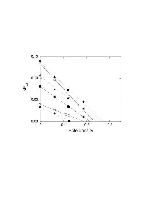
FIG. 1.: Uniform SDW energy gain per site with reference to the normal-state energy as a function of the hole density $\delta$. Data are from $8\times 8$, $10\times 10$, $12\times 12$ and $16\times 12$ systems for $\epsilon_{p}-\epsilon_{d}=2$. For solid symbols $U=4$ (circles), $U=8$ (squares), $U=12$ (triangles) and $U=20$ (diamonds) for $t_{pp}=0.2$. For open squares $U=8$ and $t_{pp}=0$ and for open squares with slash $U=8$ and $t_{pp}=0.4$. The lines are a guide to eyes. The Monte Carlo statistical errors are smaller than the size of symbols.

FIG. 2.: AF region in the plane of $U$ and the hole density for $t_{pp}=0.2$ and $\epsilon_{p}-\epsilon_{d}=2$.

FIG. 3.: Energy per site in reference to the normal state as a function of $t_{pp}$ for $16\times 4$ and $16\times 16$ lattices at $\delta=1/8$. Circles, triangles and squares denote the energy for 4-lattice stripes, 8-lattice stripes, and commensurate SDW, respectively, where $n$-lattice stripe is the incommensurate state with one stripe per $n$ ladders. In (a) the boundary conditions are antiperiodic in $x$-direction and periodic in $y$-direction, and in (b) they are periodic in $x$-direction and antiperiodic in $y$-direction. The Monte Carlo statistical errors are within the size of symbols.

III Antiferromagnetism and Stripes in the underdoped region

We show the energy gain $\Delta E_{AF}$ for the uniform SDW state in reference to the normal state for optimized parameters $g$, $\tilde{\epsilon_{p}}-\tilde{\epsilon_{d}}$ and AF order parameter $\Delta_{AF}$ in Fig.1. The energy is lowered considerably by the AF long-range ordering up to about 20of $U\approx 8-12$.

$\Delta E_{AF}$ decreases monotonically as $t_{pp}$ increases and increases as $U$ increases. One should note that $\Delta E_{AF}$ is larger than the energy gain for the $d$-wave pairing state in the low-doping region near the doping ratio $\delta\sim 0.1$ by two order of magnitude.^? The boundary of the AF state in the plane of $U$ and the hole density is shown in Fig.2 where AF denotes antiferromagnetic region. The doped holes are responsible for reducing AF correlations which leads to an order-disorder transition.

Let us look at doped systems on the two-dimensional plane with respect to modulated spin structures. Recent neutron-scattering measurements have revealed incommensurate structures suggesting stripes.^???????? The AF states with spin modulations in space have been studied for the one-band Hubbard model^????? and t-J model^??? where various stripe structures are proposed. Our purpose is to examine the possible stripe structures and their parameter dependence based on the realistic three-band Hubbard model. We can introduce a stripe in the uniform spin density state so that doped holes occupy new levels close to the original Fermi energy keeping the energy loss of AF background to a minimum.

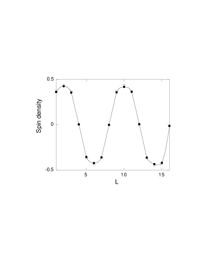
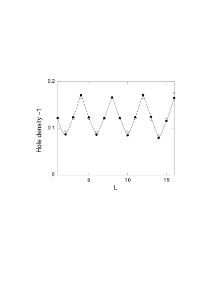
FIG. 4.: Spin density $(-1)^{\ell-1}S_{z}(\ell)$ (a) and hole density (b) functions at $\delta=1/8$ where $S_{z}(\ell)=n_{d\ell\uparrow}-n_{d\ell\downarrow}$. Solid symbols are for the $16\times 16$ square lattice and open symbols are for the $16\times 4$ rectangular lattice. The boundary conditions are antiperiodic in $x$-direction and periodic in $y$-direction, respectively.

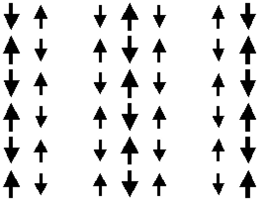
FIG. 5.: Spin structure in the incommensurate stripe state at $\delta=1/8$. The boundary conditions are the same as in Fig.4.

FIG. 6.: Energy per site in reference to the normal state as a function of $t_{pp}$ for a $16\times 16$ square lattice at $\delta=1/16$. Circles, triangles and squares denote the energy for 4-lattice stripes, 8-lattice stripes, and commensurate SDW, respectively. For solid symbols the boundary conditions are antiperiodic in $x$-direction and periodic in $y$-direction, and for open triangles they are periodic in $x$-direction and antiperiodic in $y$-direction, respectively. Monte Carlo statistical errors are smaller than the size of symbols.

FIG. 7.: Energy difference between the commensurate and incommensurate states at $\delta=1/16$ ($16\times 16$ lattice), $\delta=1/12$ ($24\times 12$ lattice) and $\delta=1/8$ ($16\times 16$ lattice). From the top $t_{pp}=0.2$, $t_{pp}=0.25$ and $t_{pp}=0.3$. The boundary conditions are periodic in $x$-direction and antiperiodic in $y$-direction, respectively.

In the actual calculations we set $\xi_{c}=1$ and $\xi_{s}=1$ in eqs.(8) and (9) since the expected values are mostly independent of $\xi_{c}$ and $\xi_{s}$. We optimize $\alpha$ in eq.(8) instead of fixing it in order to lower the expected energy value further because any eigenfunction of $H_{trial}$ can be a variational wave function. It is also possible to assume that $\delta n_{di}$ and $m_{i}$ oscillate according to the cosine curves cos($4\pi\delta x_{i}$) and cos($2\pi\delta x_{i}$), respectively, where $\delta$ is the doping ratio. Both methods give almost the same results within Monte Carlo statistical errors. Let us define $n$-lattice stripe as an incommensurate state with one stripe per $n$ ladders for which the incommensurate wave vector is given by $Q_{s}=(\pi\pm\pi/n,\pi)$ and $Q_{c}=(\pm 2\pi/n,0)$ for the spin and charge parts, respectively. The incommensurate state predicted by neutron experiments at $\delta=1/8$ is four-lattice stripe for which $Q_{s}=(\pi\pm\pi/4,\pi)$ and $Q_{c}=(\pm\pi/2,0)$. In Fig.3 we show the energy for commensurate and incommensurate SDW states on the $16\times 16$ lattice at the doping ratio $\delta$=1/8, where the incommensurability is given by $\pi/4(=2\pi\delta)$ for four-lattice stripes and $\pi/8$ for eight-lattice stripes, respectively. The four-lattice stripe is stable in the range of $0.2\leq t_{pp}\leq 0.4$. In Fig.3 we have shown the energy for two types of boundary conditions, which indicates that the effect of boundary conditions is not crucial for the $16\times 16$ system, whilst the boundary conditions change the ground state completely for small systems such as a $16\times 4$ lattice. The spin-correlation function exhibits an incommensurate structure as shown in Fig.4 and the hole-density function oscillates corresponding to a formation of stripes. The spin structures are illustrated in Fig.5. The energy at $\delta=1/16$ is shown in Fig.6 where the four-lattice stripe state has a higher energy level than for eight-lattice stripe for all values of $t_{pp}$. The energy gain of the incommensurate state per site in reference to the uniform AF state denoted as $\Delta E_{c-in}$ is shown in Fig.7 for $t_{pp}=0.2$, 0.25 and 0.3.

The incommensurability $\Delta q/(2\pi)$ for $t_{pp}=0.3$ is also shown in Fig.8 by solid circles, which is proportional to the doping ratio and is consistent with the neutron-scattering experiments for incommensurability.^? This should be compared with the variational Monte Carlo evaluations for the one-band Hubbard model^? where the stripe states with large intervals are shown to be stable. Inorder to explain the linear dependence of $\Delta q/(2\pi)$ on the hole density, the effect of $t_{pp}$ should be taken into account. The energy gain due to a formation of stripes is approximately proportional to the number of stripes. The size dependence of $\Delta E_{c-in}$ is presented in Fig.9; we observe a tendency that $\Delta E_{c-in}$ increases as the system size $N$ increases. The energy gain in the bulk limit is given by 0.002$t_{dp}\approx$ 3meV for $t_{pp}=0.3$ where $t_{dp}=1.5$eV.^???

We present typical energy scales obtained from variational Monte Carlo calculations in terms of $t_{dp}$ in Table I. The energy scales for superconductivity are consistent with experimental suggestions and energy difference $\Delta E_{c-in}$ between commensurate and incommensurate states are greater than the SC condensation energy by one order of magnitude. The commensurate AF energy gain in reference to the normal state (denoted as $\Delta E_{AF}$) is larger than $\Delta E_{AF}$ by one order of magnitude in the low-doping region.

FIG. 8.: Solid circles denote incommensurability $\Delta q/(2\pi)$ for $t_{pp}=0.3$ where the incommensurability is proportional to the hole density. For large $t_{pp}$ values the incommensurability equals zero as shown by the open circles. The boundary conditions are the same as in Fig.7.

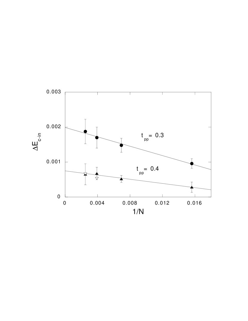
FIG. 9.: Energy difference between the commensurate and incommensurate states as a function of $1/N$ for $t_{pp}=0.3$ (circles) and $t_{pp}=0.4$ (triangles). Solid symbols are for rectangular lattices ($16\times 4$, $24\times 6$, $\cdots$), and open symbols are for square lattices ($16\times 16$, $\cdots$) The incommensurate state is assumed to be the 4-lattice stripe state. The boundary conditions are periodic in $x$-direction and antiperiodic in $y$-direction, respectively.

  

TABLE I.: Typical energy scales obtained from variational Monte Carlo calculations for $U=8$, $t_{pp}\approx 0.3$ and $\epsilon_{p}-\epsilon_{d}=2$. $\Delta_{AF}$ and $\Delta E_{AF}$ denote the magnitude of AF order parameter and the AF energy gain compared to the normal state at half-filling $\delta=0$, respectively. $\Delta_{SC}$ and $\Delta E_{SC}$ represent the optimized SC order parameter and SC energy gain at $\delta\sim 0.2$, respectively. The last column indicates experimental suggestions.

	doping ratio	Energy($t_{dp}$)	Exp.
$\Delta_{SC}$		0.01$\sim$0.015(=15$\sim$ 20meV)	10$\sim$ 20meV??
$\Delta E_{SC}$		$\sim 0.0005$(=0.75meV)??	0.17$\sim$0.26meV??
$\Delta_{AF}$	$\delta=0$	$\sim 0.6$(=900meV)
$\Delta E_{AF}$	$\delta=0$	$\sim 0.06$(=90meV)
$\Delta_{AF}$	$\delta=1/8$	$\sim 0.4$
$\Delta_{incom}$	$\delta=1/8$	$\sim 0.6$
$\Delta E_{c-in}$	$\delta=1/8$	$\sim 0.002$(=3meV)

  

IV Summary

We have presented our evaluations for the two-dimensional three-band Hubbard model using the variational Monte Carlo method. We have examined an effect produced by holes doped into the AF state in the low-doping region. The boundary of AF phase is dependent on $U$ as shown in the phase diagram in Fig.2. The inhomogeneous states with stripes are stabilized due to hole doping so that the energy loss of the AF background is kept to a minimum with the kinetic-energy gain of holes compared to uniform (commensurate) AF state. In large systems the effect of boundary conditions is reduced in our evaluations. The distance between stripes is dependent upon the transfer integral $t_{pp}$ between oxygen orbitals in the three-band model. There is a region where incommensurability is proportional to the doping ratio $\delta$ when $\delta$ is small and the energy gain due to a stripe formation is approximately proportional to the number of stripes. A linearity of the incommensurability is consistent with the neutron-scattering measurements.^? It is expected that the inhomogeneity plays an important role in the underdoped region with respect to anomalous metallic properties in high-$T_{c}$ superconductors. We have also shown the typical energy scales obtained from variational Monte Carlo calculations. It has been already established that the condensation energy $\Delta E_{SC}$ and the magnitude of order parameter for superconductivity are in reasonable agreement with the experimental results.^? The energy gain due to AF ordering is larger than $\Delta E_{SC}$ by about two order of magnitude and the energy difference between the commensurate and incommensurate states is larger than $\Delta E_{SC}$ by one order. The order of AF energy gain in reference to the normal state approximately agrees with that for the t-J model.^? Our evaluations seem to overestimate the antiferromagnetic energy because of the simplicity of the Gutzwiller wave functions, which may give a starting point for more sophisticated evaluations such as Green function Monte Carlo approaches.

References

- 1 See, for example, Proceedings of 22nd International Conference on Low Temperature Physics (LT22,Helsinki, Finland, 1999) Physica B284-288 (2000).
- 2 V.J. Emery, Phys. Rev. Lett. 58, 2794 (1987).
- 3 L.H. Tjeng, H. Eskes, and G.A. Sawatzky, Strong Correlation and Superconductivity edited by H. Fukuyama, S. Maekawa and A.P. Malozemoff (Springer, Berlin Heidelberg, 1989), pp.33.
- 4 G. Shirane, Y. Endoh, R. Birgeneau, M.A. Kastner, Y. Hidaka, M. Oda, M. Suzuki, and T. Murakami, Phys. Rev. Lett. 59, 1613 (1987).
- 5 K. B. Lyons, P.A. Fleury, L.F. Schncemmeyer, and J.V. Waszczak, Phys. Rev. Lett. 60, 732 (1988).
- 6 G. Aeppli and D.J. Buttrey, Phys. Rev. Lett. 61, 203 (1988).
- 7 E. Manousakis and R. Salvadoe, Phys. Rev. Lett. 62, 1310 (1989).
- 8 H.-Q. Ding and M.S. Makivic, Phys. Rev. Lett. 64, 1449 (1990).
- 9 F.C. Zhang and T.M. Rice, Phys. Rev. B37, 3759 (1988).
- 10 P. Prelovsek, Phys. Lett. A126, 287 (1988).
- 11 M. Inui and S. Doniach, Phys. Rev B38, 6631 (1988).
- 12 T. Yanagisawa, Phys. Rev. Lett. 68, 1026 (1992); T. Yanagisawa and Y. Shimoi, Phys. Rev. B48, 6104 (1993).
- 13 J.M. Tranquada, B.J. Sternlieb, J.D. Axe, Y. Nakamura, and S. Uchida, Nature 375, 561 (1995).
- 14 T. Nakanishi, K. Yamaji and T. Yanagisawa, J. Phys. Soc. Jpn. 66, 294 (1997).
- 15 K. Yamaji, T. Yanagisawa, T. Nakanishi and S. Koike, Physica C 304, 225 (1998).
- 16 T. Yanagisawa, S. Koike and K. Yamaji, J. Phys. Soc. Jpn. 67, 3867 (1998); ibid 68, 3867 (1999).
- 17 M. Ogata and H. Shiba, J. Phys. Soc. Jpn. 57, 3074 (1988).
- 18 W.H. Stephan, W. Linden, and P. Horsch, Phys. Rev. B39, 2924 (1989).
- 19 J.E. Hirsch, E.Y. Loh, D.J. Scalapino, and S. Tang, Phys. Rev. B39, 243 (1989).
- 20 R.T. Scalettar, D.J. Scalapino, R.L. Sugar, and S.R. White, Phys. Rev. B44, 770 (1991).
- 21 G. Dopf, A. Muramatsu, and W. Hanke, Phys. Rev. B41, 9264 (1990).
- 22 G. Dopf, A. Muramatsu, and W. Hanke, Phys. Rev. Lett.68, 353 (1992).
- 23 T. Hotta, J. Phys. Soc. Jpn. 63, 4126 (1994).
- 24 T. Asahata, A. Oguri and S. Maekawa, J. Phys. Soc. Jpn. 65, 365 (1996).
- 25 K. Kuroki and H. Aoki, Phys. Rev. Lett. 76, 4400 (1996).
- 26 T. Takimoto and T. Moriya, J. Phys. Soc. Jpn. 66, 2459 (1997).
- 27 M. Guerrero, J.E. Gubernatis and S. Zhang, Phys. Rev.B 57 , 11980 (1998).
- 28 S. Koikegami and K. Yamada, J. Phys. Soc. Jpn. 69, 768 (2000).
- 29 T. Yanagisawa, S. Koike and K. Yamaji, Physica B284, 467 (2000); B281, 933 (2000).
- 30 S. Koikegami and T. Yanagisawa, J. Phys. Soc. Jpn. 70, 3499 (2001); ibid. 71, 671 (2002) (E).
- 31 J. Zaanen and A.M. Oles, Ann. Phys. 5, 224 (1996).
- 32 T. Yanagisawa, S. Koike and K. Yamaji, in Physics in Local Lattice Distortions edited by A. Bianconi and H. Oyanagi (American Institute of Physics, New York, 2001), p. 232.
- 33 T. Yanagisawa, S. Koike and K. Yamaji, Phys. Rev. B64, 184509 (2001).
- 34 T. Giamarchi and C. Lhuillier, Phys. Rev. B43, 12943 (1991).
- 35 R. Blankenbecler, D.J. Scalapino, and R.L. Sugar, Phys. Rev. D24, 2278 (1981).
- 36 C.J. Umrigar, K.G. Wilson, J.W. Wilkins, Phys. Rev. Lett. 60, 1719 (1988).
- 37 J. Tranquada, J.D. Axe, N. Ichikawa, Y. Nakamura, S. Uchida, and B. Nachumi, Phys. Rev. B54, 7489 (1996).
- 38 J.M. Tranquada, J.D. Axe, N. Ichikawa, A.R. Moodenbaugh, Y. Nakamura, and S. Uchida: Phys. Rev. Lett. 78, 338 (1997).
- 39 T. Suzuki, T. Goto, K. Chiba, T. Fukase, H. Kimura, K. Yamada, M. Ohashi, and Y. Yamaguchi, Phys. Rev. B57, 3229 (1998).
- 40 K. Yamada, C.H. Lee, K. Kurahashi, J. Wada, S. Wakimoto, S. Ueki, H. Kimura, and Y. Endoh, Phys. Rev. B57, 6165 (1998).
- 41 M. Arai, T. Nishijima, Y. Endoh, T. Egami, S. Tajima, K. Tomimoto, Y. Shiohara, M. Takahashi, A. Garrett, and S.M. Bennington, Phys. Rev. Lett. 83, 608 (1999).
- 42 S. Wakimoto, R.J. Birgeneau, M.A. Kastner, Y.S. Lee, R. Erwin, P.M. Gehring, S.H. Lee, M. Fujita, K. Yamada, Y. Endoh, K. Hirota, and G. Shirane, Phys. Rev. B61, 3699 (2000).
- 43 M. Matsuda, M. Fujita, K. Yamada, R.J. Birgeneau, M.A. Kastner, H. Hiraka, Y. Endoh, S. Wakimoto, and G. Shirane: Phys. Rev. B62, 9148 (2000).
- 44 H.A. Mook, D. Pengcheng, F. Dogan and R.D. Hunt, Nature 404, 729 (2000).
- 45 D. Poilblanc and T.M. Rice, Phys. Rev. B39, 9749 (1989).
- 46 M. Kato, K. Machida, H. Nakanishi and M. Fujita, J. Phys. Soc. Jpn. 59, 1047 (1990).
- 47 H. Schulz, Phys. Rev. Lett. 64, 1445 (1990).
- 48 M. Ichioka and K. Machida, J. Phys. Soc. Jpn. 68, 4020 (1999).
- 49 S. White and D.J. Scalapino, Phys. Rev. Lett. 80, 1272 (1998).
- 50 S. White and D.J. Scalapino, Phys. Rev. Lett. 81, 3227 (1998).
- 51 C.S. Hellberg and E. Manousakis, Phys. Rev. Lett. 83, 132 (1999).
- 52 H. Eskes, G.A. Sawatzky, L.F. Feiner, Physica C160, 424 (1989).
- 53 M.S. Hybertson, E.B. Stechel, M. Schlüter, D.R. Jennison, Phys. Rev. B41, 11068 (1990).
- 54 A.K. McMahan, J.F. Annett, and R.M. Martin, Phys. Rev. B42, 6268 (1990).
- 55 J.R. Kirtley, C.C. Tsuei, S.I.Park, C.C. Chi, J. Rozen, M.W. Shafer, Phys. Rev. B35, 7216 (1987).
- 56 S. Kashiwaya, T. Ito, K. Oka, S. Ueno, H. Takashima, M. Koyanagi, Y. Tanaka, and K. Kajimura, Phys. Rev. B57, 8680 (1998).
- 57 J.W. Loram, K.A. Mirza, J.R. Cooper, and W.Y. Liang, Phys. Rev. Lett. 71, 1470 (1993).
- 58 P.W. Anderson, Science 279, 1196 (1998).
- 59 H. Yokoyama and M. Ogata, J. Phys. Soc. Jpn. 65, 3615 (1996).