Monte Carlo study of the elastic interaction in heteropitaxial growth

Abstract

We have studied the island size distribution and spatial correlation function of an island growth model under the effect of an elastic interaction of the form $1/r^{3}$. The mass distribution $P_{n}(t)$ that was obtained presents a pronounced peak that widens with the increase of the total coverage of the system, $\theta$. The presence of this peak is an indication of the self-organization of the system, since it demonstrates that some sizes are more frequent than others. We have treated exactly the energy of the system using periodic boundary conditions which were used in the Monte-Carlo simulations. A discussion about the effect of different factors is presented.

]

I Introduction

Epitaxial growth has been the focus of much interest in the past years. This interest is derived mainly from the fact that this kind of processes have numerous applications [1, 2, 3] in developing new types of devices and materials with some special characteristics. Among these processes, there is one type of growth characterized by the presence of long-range elastic interactions that play a special role [4]. Molecular Beam Epitaxy (MBE) under the effect of elastic interactions has been a topic of recent research, with many applications, specially in the fabrication of low dimensional nanostructures, like quantum dots (QD) and quantum wires [2, 5, 6]. One challenging question concerning this topic is how, and by which mechanism, island organization [7, 8] occurs. A wide range of material/substrate combinations have been observed (e.g., InAS on GaAs). When one kind of material is deposited over a different one –, usually, with a different lattice parameter – it will induce, through this structural difference, a long-range elastic interaction between the deposited atoms during surface growth. The deformation thus obtained originates a strain in the substrate that causes different particles to repel each other. This kind of interaction is supposed to be the mechanism responsible of the self-organization observed experimentally. Many recent studies were developed in order to identify the influence of strain on epitaxial and surface morphology during growth [9, 11, 12, 13, 14, 15, 16].

Several authors have studied the effect that strain induces on epitaxial growth on different types of systems. For instance, the effect of elastic strain on the properties of the well know Eden model[16], and for other versions of a harmonic interaction between the lattice atoms[17, 18]. Also, the Lennard-Jones potential was used to study a similar phenomena [19].

In this paper we shall consider that the strain induced on the system is due to an repulsive elastic interaction between the deposited particles proportional to $1/r^{3}$. This type of potential can be derived from elasticity theory considerations [4, 20, 21, 22, 23], when a lattice distortion is created (e.g. by cutting out a sphere of the bulk and substituting it by a different radius sphere) a field of lattice strains is created. It is already known that this type of long-range interaction can be applied to the absorption of atoms onto a surface but is only valid on the case of very thin absorbed clusters (submonolayer regime); in more general cases it can be obtained by scaling laws [15].

II Elastic Interaction Potential

We define the elastic potential to be of the form, $E=Gm_{i}m_{j}/r^{3}$, where $r$ represents the distance between the particles, $m_{i}$ is the “mass” of the particle $i$, and $G$ is the coupling constant. $G$ usually depends on the elastic properties of the substrate, such as the Young modulus, the Poisson ratio and the lattice mismatch. The coupling constant is given by [11] as being, $G=\pi(1-\sigma^{2})a^{2}f^{2}/E$, but other authors define it in different ways [4, 16]. The numerical values of the various forms differ on several orders of magnitude. We overcome this difficulty by leaving the analythical form of $G$ unspecified and determining a reasonable numerical value for it by physical considerations.

Since we are trying to study the behavior of a macroscopic material, we employed periodic boundary conditions during the simulations. The presence of this type of boundary conditions implies that some treatment must be given to the energy defined above in order to avoid some undesirable “finite-size effects” that could originate “unphysical” results. To accomplish this, we consider an infinite succession of replicas of the system and calculate the total energy of the infinite system thus obtained. The total energy has the contribution of two components, the first being the interaction energy between the particle that is currently suffering the absorption on the original system and all the other copies of this particle that belong to the other systems. This contribution is given by

$$E_{1}=\sum_{\forall i}\frac{Gm_{i}^{2}}{L^{3}}\sum_{\forall k\neq 0}\frac{1}{k^{3}}=\frac{2G\zeta(3)}{L^{3}}\sum_{\forall i}m_{i}^{2}$$ (1)

where $L$ is the linear dimension of the system and $\zeta(x)$ is the Riemman Zeta function. The first sum is performed over all particles present in the system at this time.

The second contribution to the total energy is given by the interaction between the deposited particle and all particles deposited previously in the system. This contribution is expressed as,

$$E_{2}=\sum_{i<j}\frac{Gm_{i}m_{j}}{L^{3}}\sum_{k=-\infty}^{\infty}\frac{1}{(a_{ij}+k)^{3}}.$$ (2)

where the first sum is performed over all pairs of particles, $a_{ij}$ is the distance that separates the two particles in the original system divided by $L$. Considering that

$$\sum_{k=0}^{\infty}\frac{1}{(k+a)^{3}}=-\frac{1}{2}\psi^{(2)}(a)$$ (3)

where $\psi^{(2)}(a)$ is the second order Polygamma function, and after performing some straightforward algebraic manipulations, the energy $E_{2}$ takes the following form,

$$E_{2}=\sum_{i<j}\frac{Gm_{i}m_{j}}{L^{3}}\left\{\frac{1}{a_{ij}^{3}}-\frac{1}{2}\left(\psi^{(2)}(a_{ij})+\psi^{(2)}(-a_{ij})\right)\right\}.$$ (4)

The total energy of the system is then given by

$$E_{T}=\frac{2G\zeta(3)}{L^{3}}\sum_{i}m_{i}^{2}+\\ \sum_{i<j}\frac{Gm_{i}m_{j}}{L^{3}}\left\{\frac{1}{a_{ij}^{3}}-\frac{1}{2}\left(\psi^{(2)}(a_{ij})+\psi^{(2)}(-a_{ij})\right)\right\}$$ (5)

During the simulations, and since we are not interested in the absolute value of the energy but only in energy differences, we shall only consider the “effective” value of the energy, that is, the part of the energy that is not constant, in order to shorten the CPU time without loss of precision in the results.

III Simulations

The model described earlier was implemented in a relatively simple way. We consider the substrate to be one dimensional and we shall only consider the regime of submonolayer growth. One site of the system is selected randomly. If that site is occupied, the deposition attempt fails and another site is selected. If the selected position is empty, three possible situations can occur according to the number of nearest neighbor (NN) sites that are occupied. When only one NN is occupied, the particle adheres irreversibly to the preexisting cluster and another deposition attempt is performed. If the two NN are occupied, the particle adheres to both clusters, coalescing them to become one single cluster with mass conservation. Finally, if none of the NN sites is occupied, the particle diffuses, due to the repulsive effect of the potential generated by the mass distribution present in the system, moving away from the larger cluster and becoming closer to the smaller one, until it reaches the local minimum of the energy. At each diffusion step, the energy resulting from the interaction of the adatom with every other particle present in the system is calculated. At this point, the particle begins to diffuse due to the effect of the temperature with probability proportional to $e^{-\Delta E/k_{B}T}$, where $E$ is the total energy of the system [24]. During this process, a number $D$ of random steps is performed. If during this random walk motion, the particle collides with another particle, it aggregates irreversibly and another particle is deposited. This model has several adjustable parameters such as the temperature $T$, the number of diffusion steps $D$ and the value of the interaction constant $G$. In order to make the simulations behave realistically, these parameters must be adjusted and their effect on the final result must be studied and well understood. This has been done by varying the parameters in order to see the effect that each parameter individually has on the final result. During the experimental study of this type of processes, one usually uses temperatures in the interval $300K\leq T\leq 1000K$. To use this values during the simulations, one must adjust $G$ in a way as to make the factor $\Delta E/k_{B}T\sim 1$. The typical value of the energy differences in this model is of the order $10^{9}$, and considering that $T\sim 10^{2}$ we find that $Gm^{2}\Delta E_{ef}/(L^{3}k_{B}T)\sim 1$, and so, $Gm^{2}/L^{3}k_{B}\sim 10^{-7}$.

IV Results

In this section we will present the results obtained using Monte Carlo simulations. To characterize the coarsening dynamics, two quantities were sampled and averaged over the initial conditions: cluster “mass” distribution, $P_{n}(t)$ and the correlation function at equal times $C(r,t)$, defined by

$$C(r,t)=\langle\rho(r^{\prime}+r,t)\rho(r^{\prime},t)\rangle-\langle\rho(r^{\prime},t)\rangle^{2}$$ (6)

where $\rho(r,t)$ is the site density. The most convincing result yielding the self-organization process is the fact that the “mass” distribution function presents a well defined peak.

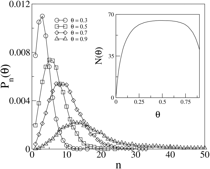
FIG. 1.: Mass distribution variation with the increase of the system coverage. Notice that the distribution function widens as the coverage increases. In the inset we represent the number of clusters present in the system as a function of coverage. It is visible that after a certain point, the number of clusters decreases due to the occurrence of coalescence phenomena. In all the simulations, $T=500K$ and $D=200$ steps.

The shape of the distribution is maintained as one increases the coverage, but the height of the function tends to decrease as the width increases. This fact was expected to happen, larger values of coverage imply that fewer individual clusters are present in the system, but with large sizes.

There exist two basic process that the system has available in order to organize itself. The first, the nucleation of new clusters, is dominant in the early stages of the system evolution, when the coverage is small and the adatoms never collide. The second, is the coalescence of existing clusters. This process becomes dominant as the coverage increases, originating larger clusters but in a smaller number. This two regimes are clearly seen in the inset of Fig.1. In the beginning, the number of clusters in the system seems to grow almost linearly with the coverage. Afterwards, there exists a crossover period when the number of clusters is approximately constant, that happens when the growth of existing clusters becomes more frequent than the nucleation of new ones. Finally, coalescence begins to dominate the dynamics and the number of clusters in the system diminishes until it becomes one when the coverage gets very large.

The behaviour of the system is described by the island-size distribution function, $P_{n}(\theta)$. Assuming there exists a scaling for $P_{n}(\theta)$ one may write, $P_{n}(\theta)=\lambda f(\lambda^{\alpha}n,\lambda^{\beta}\theta)$. The coverage $\theta$ grows with time, but satisfies, $\theta\equiv\sum_{n\geq 1}nP_{n}(\theta)$. This sum can be approximated by an integral, $\theta\approx\int_{0}^{\infty}nP_{n}(\theta)dn$ resulting a relation between the exponents, $\beta=2\alpha-1$. Therefore, one can write,

$$P_{n}(\theta)=\theta^{1-2\alpha/\beta}\Phi\left(\frac{n}{\theta^{\alpha/\beta}}\right)$$ (7)

All this results follows from the assumption that there exist only one characteristic size in the system, the average island size, $S=\sum_{n\geq 1}nP_{n}(\theta)/\sum_{n\geq 1}P_{n}(\theta)\sim\theta^{\alpha/\beta}$. The data colapse of $P_{n}(t)$ is shown in Fig.2. It was obtained for $\alpha=1.47\pm 0.05$ and $\beta=1.23\pm 0.05$.

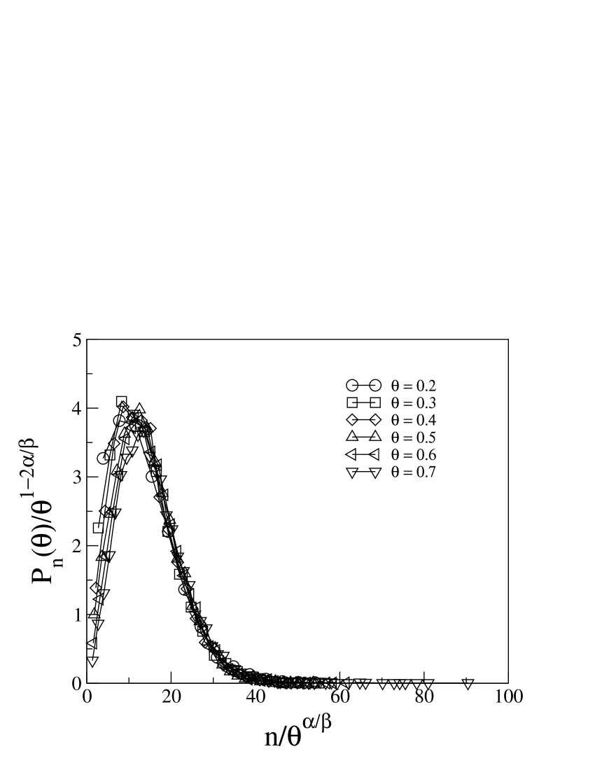
FIG. 2.: Scaling of the mass distribution function Pn(t) with the system coverage. The values of $\alpha$ and $\beta$ are respectively, 1.23 and 1.47 with an error of $0.05$ in both cases. ($T=500K$ and $D=200$)

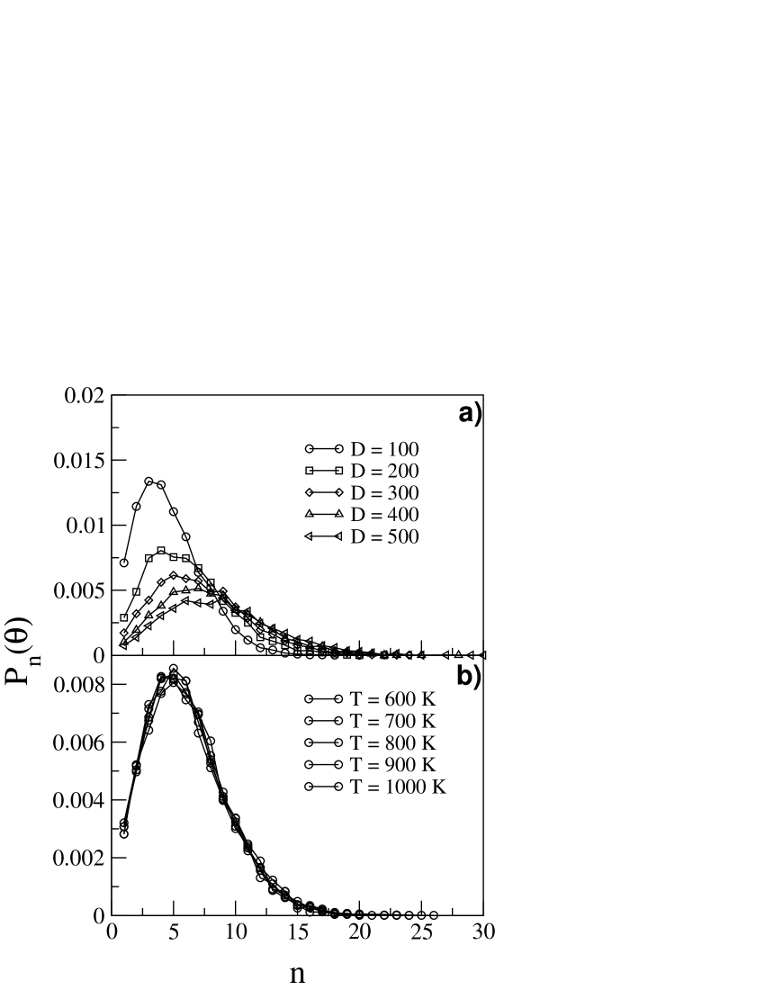
FIG. 3.: Variations in the mass distribution when the number of diffusion steps $D$ and the temperature $T$ changes. a) With the increase in $D$, the mass distribution keeps the same basic shape, but it’s width increases while it’s height decreases in a form similar to the one observed in Fig.1 when we increased the coverage of the system ($T=500$ and $\theta=0.3$). The temperature doesn’t cause any important changes in the form that the system organizes itself.($T=500K$, $\theta=0.3$)

When we keep the value of the coverage fixed and vary $D$, the mass distribution function behaves in a manner similar to the one described above. As $D$ increases, the distribution function widens and flattens. This is due to the fact that, with a larger number of diffusion steps, the adatom has a larger probability of diffusing away from the local minimum of energy and coalescing with other particles present in the system, originating larger clusters. On the other hand, when we change the temperature, nothing seems to happen, the distribution function maintains its basic properties.

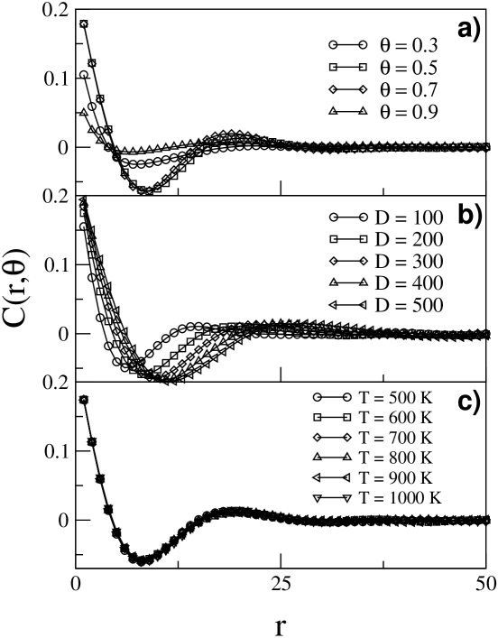
FIG. 4.: Correlation function at various coverages. In a) we observe the evolution of the correlation function as the coverage increases. It is clearly seen that the position of the minimum tends to move to larger values of r ($T=500K$ and $D=200$). b) A similar precession of the minimum is observed when $D$ is increased ($\theta=0.3$ and $T=500$). c) The correlation function doesn’t seem to be affected by the changes in T. This is probably due to the fact that only the diffusing adatom feels the effect of the temperature ($D=200$ and $\theta=0.3$).

As it can be seen in Fig4 a, the correlation function $C(r,t)$, defined in Eq.6, displays a characteristic behavior, starting at values of the order of 0.2 and decreasing until a minimum, at distances of the order of ten lattice units, and finally oscillating with decreasing amplitude around zero until it becomes effectively zero at distances of the order of 40. As it is easily seen from Fig.4, the correlation function always maintains the same shape, even when $\theta$ or $D$ are increased. In the latter case, the position of the minimum seems to move to larger distances as $D$ is increased, which means that the system becomes more correlated. Once again, the temperature doesn’t have any real effect on the results.

A parameter that usually has a great importance in experimental study of this type of systems is the temperature. As can be seen in the previous figures, the temperature doesn’t seem to have a great influence in the final result, contrary to what was expected. This peculiar behavior of the system can probably be explained by the fact that only the adatom that is being currently absorbed feels the temperature, the rest of the system being actually frozen. If we allowed the system to rearrange itself after the deposition of each particle, the temperature dependence would probably be more realistic, but the computation time required would also be much higher.

V Conclusion

In conclusion, the simulations carried in a one dimensional system in the submonolayer regime with long range interactions allowed us to observe the mechanism of self-organization through the formation of islands of similar size over all system. The influence of different factors on this behavior was tested. Surprisingly, it does not show any dependence on the temperature, at least for the tested range ($300K<T<1000K$).

Ordering occurs to minimize the repulsive elastic interactions between absorbed atoms. This self-organization breaks down when the coverage gets large which makes the adatom have less space to find an equilibrium position and makes the coalescence events become more and more frequent and finally dominate the dynamics of the system. We are now extending this results to the $2D$ case.

VI Acknowledgments

It is a pleasure to thank Serguei Dorogovtsev for collaboration in the early stage of this work. We also thank M.P. Santos for a critical reading of the manuscript. This work was funded in part by the project POCTI/1999/FIS/33141 (FCT-Portugal).

^∗ Electronic address: bgoncalves@breathe.com
^† Electronic address: jfmendes@fc.up.pt

REFERENCES

- [1] Y. Saito, Statistical Physics of Cristal Growth (World Scientific, Singapore, 1996
- [2] R. Notzel, J. Temmyo, and T. Tamamura, Nature (London)369, 131 (1994)
- [3] R. Julien, J. Kertesz, P. Meakin, and D.E Wolf, Surface Disordering: Growth, Roughening and Phase Transitions (Nova, Commack, NY, 1993)
- [4] V. I. Marchenko and A. Ya. Parshin, Sov. Phys. 52, 129 (1980)
- [5] H. Brune, M. Giovannini, K. Bromann, and K. Kern, Nature (London) 394, 451 (1998)
- [6] K. Pohl, M.C. Bartelt, J. de la Figuera, N.C. Bartelt, J. Hrbek, and R.Q. Hwang, Nature (London) 397, 238 (1999)
- [7] J.A. Floro, M.B. Sinclair, E. Chason, L.B. Freund, R.D. Twesten, R.Q. Hwang, and G.A. Lucadamo, Phys. Rev. Lett. 84, 701 (2000)
- [8] J.M. Moisson, F. Houzay, F. Barthe, L. Leprince, E. André, and O. Vatel, Appl. Phys. Lett. 64, 196 (1994)
- [9] T.R. Mattsson and H. Metiu, Appl. Phys. Lett. 64, 196 (1994)
- [10] M.Schroeder and D.E. Wolf, Surf. Sci. 375, 129 (1997)
- [11] P. Peyla, A. Vallat, C. Misbah, and H.Müller-Krumbhaar, Phys. Rev. Lett. 82, 787 (1999)
- [12] E.A. Brener, V.I.Marchenco, H.Müller-Krumbhaar, and R. Spatschek, Phys. Rev. Lett. 84, 4914 (2000)
- [13] A.-L. Barabási, Appl. Phys. Lett. 70, 2565 (1997)
- [14] J. Steinbrecher, H.Müller-Krumbhaar, E. Brener, C. Misbah, and P. Pelya, Phys. Rev. E 59, 5600 (1999)
- [15] Paolo Politi, Geneviéve Grenet, Alain Marty, Anne Ponchet and Jaques Villain, Phys. Rep 324, 272 (2000)
- [16] Yukio Saito and Heiner Müller-Krumbhaar, J. Phys. Soc. Japan 11, 3661 (1998)
- [17] Yukio Saito, Phys. Rev B 63, 45422 (2001)
- [18] Yukio Saito, J. Phys. Soc. Japan 69, 734 (2000)
- [19] Alexander Shindler, Theoretical aspects of growth on one and two dimensional strained crystal surfaces, PhD Thesis (1999)
- [20] L.D. Landau and Lifchitz, Theory of Elasticity (Editions Mir, Moscow, 1991)
- [21] J. Hardy and R. Bullough, Philos. Mag. 15, 237 (1967)
- [22] K.H. Lau and W. Kohn, Surf. Sci. 65, 607 (1977)
- [23] A.F. Andreev and Y.A. Kosevich, Sov. Phys. JETP 54, 761 (1981)
- [24] This method of implementation seems to be somewhat unphysical, but gives the same qualitative results with less computational effort that the usual method of allowing the particle to diffuse from the begining. This is due to the fact that the adatom will always tend to difuse to the local energy minimum. Our method only acellerates this process without changing the physics behind it.
- [25] D. Maroudas, L. A. Zepeda-Ruiz, and W. H. Weinberg, Appl. Phys. Lett. 73, 753 (1998)