Helium-4 Energy and Specific Heat
in Superfluid and Normal Phase

Abstract

The calculation of the ⁴He energy and specific heat is carried out in a wide temperature range within the two-time temperature Green functions approach. The approximation improving the random phase approximation is developed providing the correct behaviour of the calculated specific heat at the temperatures $0<T/T_{c}<0.65$ and $T/T_{c}>1.32$ where $T_{c}$ stands for the phase transition point.

Key words: liquid helium-4, specific heat, superfluid and normal phase.

PACS number(s): 05.70.Ce, 67.20.+k, 67.40.-w.

1 Introduction

The problem of the theoretical description for the many-boson system thermodynamics in a wide temperature range is a very curious one and still remains unsolved. Liquid ⁴He is the best example for the theretical studies because of its anomalous low-temperature behaviour. It is well-known how to obtain the thermodynamic functions in the limit $T\to 0$ (this is given by the theory of Bogoliubov [1]). The renormalization group theory also gives a fairly well results at the point of the lambda-transition [2]. But still, quite a large temperature range might be studied by means of numerical computations only.

Sears [3] utilized neutron scattering results in order to determine the internal energy of liquid helium-4 via some simple thermodynamic relations. For these calculations, the potential of Aziz et al [4] was used for representing the He–He interatomic interaction.

Path Integral Monte Carlo (PIMC) technique which allows for the study of the physical quntities temperature dependences was utilized by Ceperley and Pollock [5] for the helium-4 thermodynamic properties calculation at the temperatures above 1 K. Kinetic energy of liquid and solid helium-4 was calculated in [6] at high temperatures. Such numerical simulations are numerous and we do not intend to analize them here. The overview of Path Integral Monte Carlo (PIMC) techniques application in the theory of condensed helium is adduced in the paper by Ceperley [7].

The derivation of the analytical relations for the thermodynamic properties was made by Vakarchuk [11]. In the first of the cited works, the expression for the many-boson two-particle density matrix was written. The second work contains the analysis of the non-linear density fluctuations contribution into the thermodynamic properties of the Bose-system. The expressions found there are expected to provide a good description in a wide temperature range.

In this work, we will proceed from a very well studied random phase approximation (RPA) which allows one to receive a low-temperature asymptotics for the thermodynamic and structure functions of liquid ⁴He. Then, making some quite natural assumptions, we will develop what might be called ‘effective post-RPA’ since the post-RPA corrections will be taken into account in an effective manner. In principle, such a technique will move us substantially ahead form the low-temperature region. But unfortunately the way of the equations solution applied here does not allows to grasp the temperatures $|T/T_{c}-1|\lesssim 1/3$ where $T_{c}$ stands for the lambda-transition point, this seems to be rather a technical problem.

In this paper, we use the previously obtained potential [8] for the calculation of thermodynamic properties of liquid helium. A two-time temperature Green function technique will be utilized for the calculation of the energy and specific heat. The application of this technique is well-known, it was used by Tserkovnikov [9] for the non-ideal Bose-gas in the random phase approximation. Additionally, this method leads to a quite short way to the RPA (Bogoliubov’s) results. Unlike what is usualy done, the collective variables being the density fluctuations Fourier components are utilized for constructing the Green functions instead of the creation–annihilation operators.

The organization of the paper is as follows. In Section II, we introduce the operators for the Green functions and write the Hamiltonian. In Section III, the equations of motion are written and solved. Next, the function $\gamma_{k}(T)$ for the accounting of post-RPA terms is introduced. The equations for it are adduced in Section IV. Also, the expression for the free energy is written and other thermodynamic functions are derived from it in this Section. The discussion is presented in Section V.

2 Collective variables and Hamiltonian

We consider operators

$$\rho_{\bf k} = {1\over\sqrt{N}}\sum_{j=1}^{N}e^{-i{\bf k}{\bf r}_{j}},$$ (1)

$$\hat{\pi}_{\bf k} = {1\over\sqrt{N}}\sum_{j=1}^{N}e^{-i{\bf k}{\bf r}_{j}}\left({-i\hbar^{2}\over m}{\bf k}\mbox{\boldmath{$\nabla$}}_{j}\right),$$ (2)

$$\hat{\xi}_{\bf k} = {1\over\sqrt{N}}\sum_{j=1}^{N}e^{-i{\bf k}{\bf r}_{j}}\left({-i\hbar^{2}\over m}{\bf k}\mbox{\boldmath{$\nabla$}}_{j}\right)^{2},$$ (3)

the operators $\rho_{\bf k}$ being collective variables, operators $\hat{\pi}_{\bf k}$ are usually known as ‘currents’. No special name will be given to $\hat{\xi}_{\bf k}$.

The Hamiltonian $\hat{H}$ of the system is written as $\hat{H}=\hat{H}^{(0)}+\Delta\hat{H}$ where $\hat{H}^{(0)}$ corresponds to RPA and $\Delta\hat{H}$ is the respective correction. Hereafter we will consider only RPA term and therefore use $\hat{H}$ to designate $\hat{H}^{(0)}$:

$$\hat{H}=\hat{K}+\hat{\Phi}$$ (4)

where $\hat{K}$ and $\hat{\Phi}$ being the kinetic and potential energy in RPA respectively.

We have the following expression for the potential energy operator in $\rho$-representation:

$$\hat{\Phi}={N(N-1)\over 2V}\nu_{0}+\sum_{{\bf k}\neq 0}{N\over 2V}\nu_{k}\left(\rho_{{\bf k}}\rho_{-{\bf k}}-1\right),$$ (5)

where $\nu_{k}$ means the Fourier transformation of the interatomic potential in helium [8], while the kinetic energy is given in a usual way:

$$\hat{K}=-{\hbar^{2}\over 2m}\sum_{j=1}^{N}\mbox{\boldmath{$\nabla$}}_{j}^{2}.$$ (6)

It is interesting as well to consider the $\rho$-representation for $\hat{K}$. Neglecting terms with two sums over the wave vector (i. e., leaving the RPA term only) we obtain

$$\hat{K}_{\rho}=\sum_{{\bf k}\neq 0}\left\{{1\over 2}\rho_{-{\bf k}}\hat{\pi}_{{\bf k}}-{1\over 4\varepsilon_{k}}\hat{\pi}_{-{\bf k}}\hat{\pi}_{{\bf k}}\right\},$$ (7)

$\varepsilon_{k}$ is the energy of a free particle:

$$\varepsilon_{k}={\hbar^{2}k^{2}\over 2m}.$$

3 Equations of motion for Green functions

Since the total energy of the system $E$ is the average value of the Hamiltonian we need to know the way of averaging our expressions. In order to find the average values of such expressions as $\rho_{{\bf k}_{1}}\rho_{{\bf k}_{2}}$, $\hat{\pi}_{{\bf k}_{1}}\rho_{{\bf k}_{2}}$, etc. we will use two-time temperature Green functions [10]:

$$\langle\!\langle A(t)|B(t^{\prime})\rangle\!\rangle=i\theta(t-t^{\prime})\langle[A(t),B(t^{\prime})]\rangle$$ (8)

with operators given in the Heisenberg representation, $\theta$ is the Heaviside step function. The following designations will be used:

$$G_{\rho\rho}({\bf k}_{1},{\bf k}_{2})\equiv\langle\!\langle\rho_{{\bf k}_{1}}\,|\,\rho_{{\bf k}_{2}}\rangle\!\rangle,\quad G_{\rho\pi}({\bf k}_{1},{\bf k}_{2})\equiv\langle\!\langle\rho_{{\bf k}_{1}}\,|\,\hat{\pi}_{{\bf k}_{2}}\rangle\!\rangle,\quad\ldots\,.$$ (9)

The averaging might be symbolically represented by an operator $\,\,\hat{\!\!\cal{{A}}\,}$:

$$\langle AB\rangle=\,\,\hat{\!\!\cal{{A}}\,}G_{BA}.$$ (10)

We consider here only the case of ${\bf k}_{2}=-{\bf k}_{1}\equiv{\bf k}$ since such expressions appear in our Hamiltonian (5), (7). Therefore, the indexing of ${\bf k}_{1}$, ${\bf k}_{2}$ will be skipped for the sake of simplicity.

3.1 $\rho$-representation for the kinetic energy

It is easy to show that one can obtain the following equations of motion

$$\hbar\omega\,G_{\rho\rho}(\omega) = -\varepsilon_{k}\,G_{\rho\rho}(\omega)+G_{\pi\rho}(\omega),$$

$$\hbar\omega\,G_{\pi\rho}(\omega) = {\phantom{-}}\varepsilon_{k}\,G_{\pi\rho}(\omega)+\varepsilon_{k}^{2}(\alpha_{k}^{2}-1)\,G_{\rho\rho}(\omega)+{1\over\pi}\varepsilon_{k},$$ (11)

where

$$\alpha_{k}=\sqrt{1+{2\varrho\nu_{k}\over\varepsilon_{k}}},\qquad\varrho={N\over V}.$$ (12)

Using the solutions of the above system we receive the following mean values

$$\langle\rho_{-{\bf k}}\rho_{{\bf k}}\rangle \equiv \,\,\hat{\!\!\cal{{A}}\,}G_{\rho\rho}({\bf k})\equiv S_{k}={1\over\alpha_{k}}\coth{\varepsilon_{k}\alpha_{k}\over 2T},$$

$$\langle\rho_{-{\bf k}}\hat{\pi}_{{\bf k}}\rangle \equiv \,\,\hat{\!\!\cal{{A}}\,}G_{\pi\rho}({\bf k})\equiv{\sl\widetilde{\Pi}}_{k}={1\over 2}\left({1\over\alpha_{k}}\coth{\varepsilon_{k}\alpha_{k}\over 2T}-1\right)={1\over 2}\left(S_{k}-1\right),$$

$$\langle\hat{\pi}_{-{\bf k}}\hat{\pi}_{{\bf k}}\rangle \equiv \,\,\hat{\!\!\cal{{A}}\,}G_{\pi\pi}({\bf k})\equiv{\sl\Pi}_{k}={1-\alpha_{k}^{2}\over 4\alpha_{k}}\coth{\varepsilon_{k}\alpha_{k}\over 2T}={1-\alpha_{k}^{2}\over 4}\,S_{k}.$$ (13)

Here, the average $\langle\rho_{{\bf k}}\rho_{-{\bf k}}\rangle$ is nothing but the structure factor of the system.

3.2 Exact kinetic energy

In this case, the equations of motion read:

$$\hbar\omega\,\bar{G}_{\rho\rho}(\omega) = -\varepsilon_{k}\,\bar{G}_{\rho\rho}(\omega)+\bar{G}_{\pi\rho}(\omega),$$

$$\hbar\omega\,\bar{G}_{\pi\rho}(\omega) = -\varepsilon_{k}\,\bar{G}_{\pi\rho}(\omega)+\varepsilon_{k}^{2}(\alpha_{k}^{2}-1)\,\bar{G}_{\rho\rho}(\omega)+\bar{G}_{\xi\rho}(\omega)+{1\over\pi}\varepsilon_{k}.$$ (14)

Unlike the previous case when the kinetic energy operator was given in the $\rho$-representation, now it turned to be imposible to solve this system with respect to $\bar{G}_{\rho\rho}$ even in the RPA. The problem lies in the appearence of the functions with the higher orders of $(-i\hbar^{2}\mbox{\boldmath{$\nabla$}}/m)$ in each equation following the equation for $\bar{G}_{\xi\rho}$, etc., compare with (3.1). Therefore, one should apply some approximation in order to obtain the closed system of the equations of motion.

Let us consider the system of two equations for the functions $\bar{G}_{\rho\rho}$ and $\bar{G}_{\pi\rho}$ making a suggestion that

$$\bar{G}_{\xi\rho}-2\varepsilon_{k}\,\bar{G}_{\pi\rho}=2\gamma_{k}(T)\varepsilon_{k}^{2}\,\bar{G}_{\rho\rho},$$ (15)

with the factor of $\gamma_{k}(T)$ being of the energy dimension. Its form will be choosed further.

Such a substitution returs us to system (3.1) but the quantity $\alpha_{k}$ looks different now, we will refer it as $\bar{\alpha}_{k}$:

$$\bar{\alpha}_{k} = \sqrt{1+{2\varrho\nu_{k}\over\varepsilon_{k}}+{2\gamma_{k}(T)\over\varepsilon_{k}}}$$ (16)

One should keep in mind that a bar over a letter means ‘exect with respect to RPA’.

3.3 General properties of $\gamma_{k}(T)$.

Let us consider the cases of low and high temperatures.

In the low-temperature limit the results obtained in $\rho$-representation are correct (the theory of Bogoliubov). Thus,

$$\gamma_{k}(T)\biggr{|}_{T\to 0}=0.$$ (17)

In the high-temperature limit, one has the expression for the structure factor:

$$S_{k}(T)\biggr{|}_{T\to\infty}={1\over 1+\varrho\nu_{k}/T}.$$ (18)

It leads to

$$2\gamma_{k}(T)\biggr{|}_{T\to\infty}=2T={4\over 3}K,$$ (19)

where $K$ is the kinetic energy per particle, in the high-temperature limit it equals to the classical expression $K=3T/2$.

4 Equation for $\gamma_{k}(T)$ and calculation of energy

One can calculate the free energy of the system using the expression [11]

$$F=F_{0}+\int_{0}^{1}d\lambda\,\Phi(\lambda),$$ (20)

$F_{0}$ is the free energy of non-interacting system, $\lambda$ is the ‘interaction turn-on’ parameter, $\Phi$ is the potential energy given by

$${\Phi\over N}={\varrho\nu_{0}\over 2}+{1\over 2N}\sum_{{\bf k}\neq 0}\varrho\nu_{k}\left({1\over\bar{\alpha}_{k}}\coth{\beta\over 2}\varepsilon_{k}\bar{\alpha}_{k}-1\right)$$ (21)

In order to integrate $\Phi(\lambda)$ in (20) we will use the integration over $\bar{\alpha}_{k}$ instead of $\lambda$. This involves the derivative $\partial\gamma_{k}/\partial\lambda$. One cannot found it without knowing the explicit dependence $\gamma_{k}(\lambda)$. In this situation, the most simple way is to use the method from [12] and to write the so called first difference:

$${\partial\gamma_{k}\over\partial\lambda}={\gamma_{k}-\gamma^{0}_{k}\over\Delta\lambda}=\gamma_{k}-\gamma^{0}_{k}$$ (22)

since $\Delta\lambda=1$. Here, $\gamma^{0}_{k}$ is the quantity $\gamma_{k}$ for the ideal Bose-gas.

4.1 Low temperatures, $T<T_{\lambda}$

A self-consistent relation for obtaining the quantity $\gamma_{q}(T)$ might be sketched as follows:

$$\framebox{$\begin{array}[]{l}{\rm Energy\ received}\\ {\rm from\ the\ averaged}\\ {\rm RPA{\textrm{-}}Hamiltonian}\end{array}$}\qquad=\qquad\framebox{$\begin{array}[]{l}{\rm Energy\ calculated}\\ {\rm from\ the\ free\ energy}\\ {\rm as}\ \ E=\displaystyle{\partial\;\beta F\over\partial\beta}\end{array}$}\ .$$ (29)

One should remember that every RPA-expression contains $\bar{\alpha}_{k}$ with $\gamma_{k}(T)$.

The left-hand side of the equation (29) equals

$${E\over N}={\varrho\nu_{0}\over 2}+{1\over N}\sum_{{\bf k}\neq 0}\left\{\left({1\over 2}{\sl\widetilde{\Pi}}_{k}-{1\over 4\varepsilon_{k}}{\sl\Pi}_{k}\right)+{1\over 2}\varrho\nu_{k}(S_{k}-1)\right\},$$ (30)

where relation (3.1) is taken into account.

One has for the free energy:

$${F\over N} = {F_{0}\over N}+{\varrho\nu_{0}\over 2}+{1\over 2N}\sum_{{\bf k}\neq 0}\varrho\nu_{k}\left\{{\varepsilon_{k}(\bar{\alpha}_{k}-\bar{\alpha}^{0}_{k})\over\varrho\nu_{k}+\gamma_{k}-\gamma^{0}_{k}}-1+{}\right.$$ (31)

$$\qquad\left.{}+{2T\over\varrho\nu_{k}+\gamma_{k}-\gamma^{0}_{k}}\ln{1-\exp\left(-\beta\varepsilon_{k}\bar{\alpha}_{k}\right)\over 1-\exp\left(-\beta\varepsilon_{k}\bar{\alpha}^{0}_{k}\right)}\right\}.$$

As a result, relation (29) is rewritten as follows:

$${\varrho\nu_{0}\over 2}+{1\over 2N}\sum_{{\bf k}\neq 0}\left[\left(\varepsilon_{k}\alpha_{k}-{\gamma_{k}\over\bar{\alpha}_{k}}\right)\coth{\varepsilon_{k}\bar{\alpha}_{k}\over 2T}-\varepsilon_{k}-\varrho\nu_{k}\right]=$$

$$\qquad=K_{0}(T)+{\varrho\nu_{0}\over 2}+{1\over 2N}\sum_{{\bf k}\neq 0}\varrho\nu_{k}\left\{{2(\gamma^{0}_{k}{}^{\prime}-\gamma_{k}^{\prime})\over(\varrho\nu_{k}+\gamma_{k}-\gamma^{0}_{k})^{2}}\ln{\sinh{\beta\over 2}\varepsilon_{k}\bar{\alpha}_{k}\over\sinh{\beta\over 2}\varepsilon_{k}\bar{\alpha}^{0}_{k}}+{}\right.$$

$$\qquad{}+{\varepsilon_{k}\over\varrho\nu_{k}+\gamma_{k}-\gamma^{0}_{k}}\left[\left(\bar{\alpha}_{k}-\beta\bar{\alpha}_{k}^{\prime}\right)\coth{\beta\over 2}\varepsilon_{k}\bar{\alpha}_{k}-\left(\bar{\alpha}^{0}_{k}-\beta\bar{\alpha}^{0}_{k}{}^{\prime}\right)\coth{\beta\over 2}\varepsilon_{k}\bar{\alpha}^{0}_{k}-1\right]\left.\vphantom{\ln{\sinh{\beta\over 2}\varepsilon_{k}\bar{\alpha}_{k}\over\sinh{\beta\over 2}\varepsilon_{k}\bar{\alpha}^{0}_{k}}}\right\},$$ (32)

where primes mean derivation over $\beta$ and

$$\bar{\alpha}^{0}_{k}=\sqrt{1+{2\gamma^{0}_{k}(T)\over\varepsilon_{k}}}.$$ (33)

For the $\bar{\alpha}_{k}$, $\bar{\alpha}^{0}_{k}$ derivatives we obtain:

$$\bar{\alpha}_{k}^{\prime}={\gamma_{k}^{\prime}\over\varepsilon_{k}\bar{\alpha}_{k}},\qquad\bar{\alpha}^{0}_{k}{}^{\prime}={\gamma^{0}_{k}{}^{\prime}\over\varepsilon_{k}\bar{\alpha}^{0}_{k}}.$$ (34)

The quantity $\gamma^{0}_{k}$ still remains unknown. We will try to find it utilizing the thermodynamic relations for the ideal Bose-gas.

Let us consider an arbitrary (no matter, interacting or non-interacting) system first. Its structure factor in the long-wave limit reads:

$$S_{k}(T)\bigg{|}_{k\to 0}=\lim_{k\to 0}{1\over\bar{\alpha}_{k}}\coth{\beta\over 2}\varepsilon_{k}\bar{\alpha}_{k}={T\over\varepsilon_{0}+\varrho\nu_{0}+\gamma_{0}}.$$ (35)

The expression $\varepsilon_{0}$ obviously equals to zero but we reserve it in the sence of the limit $k\to 0$, this will be necessary for the ideal gas case. Therefore,

$$\gamma_{0}={T\over S_{0}(T)}-\varrho\nu_{0}-\varepsilon_{0}={1\over\varrho\varkappa_{T}}-\varrho\nu_{0}-\varepsilon_{0},$$ (36)

where the connection between structure factor at $k=0$ and the isothermic compressibility $\varkappa_{T}$ is taken into account. For the ideal gas $\nu_{k}=0$, thus at low temperatures one receives:

$$\gamma^{0}_{0}=\left(\partial P_{0}\over\partial\varrho\right)_{T}=0\quad{\rm for}\quad T<T_{c},$$ (37)

where $P_{0}$ is the ideal Bose-gas pressure and $T_{c}$ is the Bose-condensation temperature. As a result, the ideal Bose-gas structure factor $S^{0}_{k}$ reads:

$$S^{0}_{k}(T)\biggr{|}_{k\to 0}={2\over\varepsilon_{k}}\propto{1\over k^{2}},$$ (38)

as it should be [13].

Now, we accept for the simplicity that the dependences on the wave vector and the temperature in quantities $\gamma_{k}$ and $\gamma^{0}_{k}$ separate:

$$\gamma_{k}(T)=\gamma(T)f_{k},\quad\gamma^{0}_{k}(T)=\gamma^{0}(T)f^{0}_{k},\qquad f_{0}=f^{0}_{0}=1.$$ (39)

Te above statement means the separation of the ‘primary’ temperature dependence in the comparison with the ‘secondary’ dependence on the wave vector. The latter will be integrated up when calculating the thermodynamic properties. The condition $f_{0}=f^{0}_{0}=1$ is nothing but the specific normalization condition.

Now, from $\gamma^{0}_{0}=0$ one obtains $\gamma^{0}=0$ and, taking (34) into account, also $\gamma^{0}_{k}{{}^{\prime}}=0$, $\bar{\alpha}^{0}_{k}{{}^{\prime}}=0$. These equalities are valid for $T<T_{c}$.

Let us consider the expansion of (4.1) in terms of $\gamma$ in order to obtain the equation for $\gamma_{k}(T)$. The first-order terms read:

$$T\dot{\gamma}(T)\int_{0}^{\infty}k^{2}f_{k}\left\{{2T\over\varrho\nu_{k}}\ln{\sinh{\varepsilon_{k}\alpha_{k}\over 2T}\over\sinh{\varepsilon_{k}\over 2T}}-{1\over\varrho\nu_{k}}\coth{\varepsilon_{k}\alpha_{k}\over 2T}\right\}+{}$$ (40)

$${}+\gamma(T)\int_{0}^{\infty}k^{2}f_{k}\left\{{1\over\alpha_{k}}\coth{\varepsilon_{k}\alpha_{k}\over 2T}+{\varepsilon_{k}\over\varrho\nu_{k}}\left[\coth{\varepsilon_{k}\over 2T}-\alpha_{k}\coth{\varepsilon_{k}\alpha_{k}\over 2T}\right]\right\}=0,$$

where the dot denotes the derivative with respect to the temperature and $\alpha_{q}$ is defined by the Bogoliubov’s expression (12)

Similar expansion for energy (30) leads to the following equation:

$$E = {1\over 4\pi^{2}\varrho}\int_{0}^{\infty}dk\,k^{2}\varepsilon_{k}\left[\alpha_{k}\coth{\varepsilon_{k}\alpha_{k}\over 2T}-{\alpha_{k}^{2}+1\over 2}\right]-\gamma{1\over 4\pi^{2}\varrho}\int_{0}^{\infty}dk\,k^{2}f_{k}{1\over 2T}\varepsilon_{k}{1\over\sinh^{2}{\varepsilon_{k}\alpha_{k}\over 2T}}$$

$$+ \gamma^{2}{1\over 4\pi^{2}\varrho}\int_{0}^{\infty}dk\,k^{2}\,f_{k}^{2}\Biggl{\{}{1\over 4T{\alpha_{k}}}\left[{1\over\alpha_{k}}+{\varepsilon_{k}\coth{\varepsilon_{k}\alpha_{k}\over 2T}\over T}\right]{1\over\sinh^{2}{\varepsilon_{k}\alpha_{k}\over 2T}}+{1\over 2T\varepsilon_{k}{\alpha_{k}}^{3}}\coth{\varepsilon_{k}\alpha_{k}\over 2T}\Biggr{\}}$$

The last item in the second integral causes some difficulties since it does not converge at $k\to\infty$. One can ensure the convergence by means of the function $f_{k}$ (it is arbitrary by now). The next problem with this item is the incorrect behaviour of the heat capacity at low temperatures. As it will be shown further, $\gamma(T)$ is proportional to $T$ when $T\to 0$. It leads to the linear temperature dependence of heat capacity while one should have $\propto T^{3}$. We can avoid this problem by choosing $f_{k}$ in the special form. We will demand the following:

$$\int^{\infty}_{0}dk\,k^{2}\,f_{k}^{2}\,{1\over\varepsilon_{k}\alpha_{k}^{3}}=0.$$ (42)

The similar problem is with $\gamma^{3}$ giving quadratic dependence with respect ot $T$. Thus, the second equation:

$$\int^{\infty}_{0}dk\,k^{2}\,f_{k}^{3}\,{1\over\varepsilon_{k}^{2}\alpha_{k}^{5}}=0.$$ (43)

Only a complex $f_{k}$ can satisfy both these equation. For the sake of simplicity in calculations we have choosed $f_{k}$ in the following form:

$$f_{k}=\left\{\begin{array}[]{cl}1,&0\leq k<k_{1},\\ if_{\rm II},&k_{1}\leq k<k_{2},\\ -f_{\rm III},&k_{2}\leq k<k_{3},\\ -if_{\rm IV},&k_{3}\leq k<k_{4},\\ 0,&{\rm otherwise}\end{array}\right.$$ (49)

with equally spaced intervals, $k_{n}=n\times 2$ Å^-1. Three quantities $f_{\rm II},f_{\rm III},f_{\rm IV}$ are necessary to satisfy both real and complex terms in the equations (42–43).

The equation for $\gamma$ might be rewritten as follows:

$$a_{1}(T)\,T\dot{\gamma}+a_{0}(T)\gamma+O(\gamma^{2})=0$$ (50)

Neglecting higher-order terms one obtains:

$$\gamma(T)=CT\exp\left\{-\int^{T}{d\tau\over\tau}\left[{a_{0}(\tau)\over a_{1}(\tau)}+1\right]\right\},$$ (51)

where the constant $C$ is unknown yet. One can define it studying the behaviour of the isothermic compressibility near the absolute zero (36). We received the following value by averaging the results of the data [14] interpolation at the lowest temperatures over four, five and six points:

$$C\equiv\dot{\gamma}(0)\simeq 6.6\,.$$ (52)

The $\gamma(T)$ curve is adduced at Fig. 1.

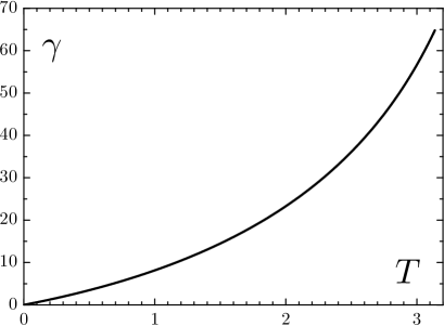
Figure 1: The dependence of $\gamma$ on the temperature.

One should notice that teh correct results must be expected only for the temperatures at which it is possible to neglect the higher-order terms in the equation for $\gamma_{k}$ (40). In other words, if $2\gamma_{k}/\varepsilon_{k}>1$ then the results are not correct. Taking into account that the typical wave vector absolute value for ⁴He is 2 Å (it corresponds to the first maximum on the structure factor curve) we obtain the upper limit for the applicability of our results as $T/T_{c}\simeq 2/3$.

4.2 High temperatures, $T>T_{\lambda}$

In this case one can use the techniques similar to the described in the previous sections for low temperatures. Unfortunately, this seems to be a rather complicated problem. Firstly, the function $\gamma^{0}_{k}(T)$ is not equal to zero already. Secondly, the quantity $\gamma_{k}(T)$ is not small in this temperature region and it is not possible to use the expansion into series, we also did not manage to solve equation (4.1) (the initial condition for the differential equation is unknown). Therefore, for the simplification of the calculations we decided to substitute $\gamma_{k}(T)$ with $2K/3$, see (19), where $K$ is the kinetic energy per particle.

We have rewritten the expression for the free energy (31) in order to obtain the equation for $\Delta K\equiv K-K_{0}$:

$$\Delta K = {1\over 4\pi^{2}}\int_{0}^{\infty}dk\,k^{2}\ \nu_{k}\Biggl{\{}{1\over Z_{k}}\varepsilon_{k}\left[\alpha_{k}\coth{\beta\over 2}\varepsilon_{k}\alpha_{k}-\alpha_{k}^{0}\coth{\beta\over 2}\varepsilon_{k}\alpha_{k}^{0}\right]-{1\over\alpha_{k}}\coth{\beta\over 2}\varepsilon_{k}\alpha_{k}$$ (53)

$$\qquad+{2\over 3}\,{\partial\Delta K\over\partial T}\Biggl{[}{T\over Z_{k}^{2}}\varepsilon_{k}(\alpha_{k}-\alpha_{k}^{0})-{T\over Z_{k}}{1\over\alpha_{k}}\coth{\beta\over 2}\varepsilon_{k}\alpha_{k}$$

$$\qquad\qquad+{2T^{2}\over Z_{k}^{2}}\Biggl{(}\ln\left(1-e^{-\beta\varepsilon_{k}\alpha_{k}}\right)-\ln\left(1-e^{-\beta\varepsilon_{k}\alpha_{k}^{0}}\right)\Biggr{)}\Biggr{]}$$

$$\qquad+{2\over 3}\dot{K}_{0}{T\over Z_{k}}\Biggl{[}{1\over\alpha_{k}^{0}}\coth{\beta\over 2}\varepsilon_{k}\alpha_{k}^{0}-{1\over\alpha_{k}}\coth{\beta\over 2}\varepsilon_{k}\alpha_{k}\Biggr{]}\Biggr{\}},$$

$$Z_{k} = \varrho\nu_{+}{2\over 3}\Delta K,$$

$$\alpha_{k} = \sqrt{1+{2\varrho\nu_{k}\over\varepsilon_{k}}+{4\over 3}{\Delta K+K_{0}\over\varepsilon_{k}}},$$

$$\alpha_{k}^{0} = \sqrt{1+{4\over 3}{K_{0}\over\varepsilon_{k}},}$$

where the dot means derivation with respect to $T$: $\dot{K}_{0}=\partial K/\partial T$.

Having calculated the kinetic energy form Eq. (53) we then proceed to the calculation of the total energy. After the numerical derivation of the latter we receive the specific heat of the liquid helium. This result is adduced in Fig. 2 together with the data for the low temperatures from the previous subsection.

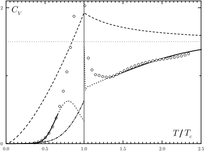
Figure 2: Energy of liquid helium-4. Solid line — calculated energy, dotted line shows the regions where the approximations used cannot be accepted; dashed line — energy of ideal Bose-gas; dashed-dotted line — Bogoliubov’s approximation.

5 Discussion

As one can see from Fig. 2 we obtained a fairly good description in the region $0\leq T/T_{c}<0.65$, as it was expected. In the normal phase ($T>T_{c}$) a similar situation is received for the temperatures $T/T_{c}>1.32$. It is necessary to say that the phase transition temperature $T_{c}$ in our case coincides with the respective temperature of the ideal Bose-gas. One should use the effective mass $m^{*}$ of the helium atom instead of that of free atom $m=4.0026$ a. m. u. As will be shown elsewhere [15], it is possible to receive the effective mass in a sel-consistent manner within the Green function formalism. The ground-state ($T=0$ K) value equals to $m^{*}\simeq 1.58\,m$. We assume that the temperature dependence of the effective mass is significant in the temperature region under consideration: $m^{*}(T)\simeq{\rm const}=m^{*}(0)=1.58\,m$. Therefore, one receives the transition temperature of 1.99 K vs experimental 2.17 K [15].

References

- [1] N. N. Bogoliubov, Izv. AN SSSR, ser. fiz. 11, 77 (1947) [in Russian].
- [2] H. Kleinert, Phys. Lett. A 277, 205 (2000).
- [3] V. F. Sears, Phys. Rev. B 28, 5109 (1983).
- [4] R. A. Aziz, V. P. S. Nain, J. S. Carley, W. L. Taylor, G. T. McConville, J. Chem. Phys. 70, 4430 (1979).
- [5] D. M. Ceperley, E. L. Pollock, Phys. Rev. Lett. 56, 351 (1986).
- [6] D. M. Ceperley, R. O. Simmons, R. C. Blasdell, Phys. Rev. Lett. 77, 115 (1996).
- [7] D. M. Ceperley, Rev. Mod. Phys. 67, 279 (1995).
- [8] I. O. Vakarchuk, V. V. Babin, A. A. Rovenchak, J. Phys. Stud. (Lviv) 4, 16 (2000).
- [9] Yu. A. Tserkovnikov, DAN SSSR 159, 1023 (1964) [in Russian].
- [10] D. N. Zubarev, Neravnovesnaia statisticheskaia termodinamika (Nauka, Moscow, 1971) [in Russian]; D. N. Zubarev, Nonequilibrium statistical thermodynamics (Consultants Bureau, New York, 1974).
- [11] I. O. Vakarchuk, J. Phys. Stud. (Lviv) 1, 156 (1997); 3, 264 (1999) [in Ukrainian].
- [12] I. O. Vakarchuk, Vstup do problemy bahatiokh til (Introduction into the Many-Body Theory) (Lviv University Publisher, Lviv, 1999) [in Ukrainian].
- [13] N. N. Bogoliubov, Izbrannye trudy v trekh tomakh. T. 3 (Selected Works in Three Volumes. Vol. 3) (Naukova dumka, Kiev, 1971), p. 216 [in Russian].
- [14] V. D. Arp, R. D. McCarty, D. G. Friend, Natl. Inst. Stand. Technol. Tech. Note 1334 (revised) (1998).
- [15] A. Rovenchak, preprint cond-mat/0203484.