Nonequilibrium relaxation in neutral BCS superconductors:
Ginzburg-Landau approach with Landau damping in real time

Abstract

We present a field-theoretical method to obtain consistently the equations of motion for small amplitude fluctuations of the order parameter directly in real time for a homogeneous, neutral BCS superconductor. This method allows to study the nonequilibrium relaxation of the order parameter as an initial value problem. We obtain the Ward identities and the effective actions for small phase the amplitude fluctuations to one-loop order. Focusing on the long-wavelength, low-frequency limit near the critical point, we obtain the time-dependent Ginzburg-Landau effective action to one-loop order, which is nonlocal as a consequence of Landau damping. The nonequilibrium relaxation of the phase and amplitude fluctuations is studied directly in real time. The long-wavelength phase fluctuation (Bogoliubov-Anderson-Goldstone mode) is overdamped by Landau damping and the relaxation time scale diverges at the critical point, revealing critical slowing down.

I Introduction

Nonequilibrium phenomena in superconductors continue to be the focus of attention. The dynamics of Josephson junctions, phase slip phenomena in the dynamics of vortices and relaxation of the order parameter and supercurrents are few examples of the experimental effort that probe nonequilibrium aspects of superconductivity.

Since the original work of Abrahams and Tsuneto tsuneto there has been an ongoing effort in trying to obtain the effective time-dependent description of nonequilibrium phenomena from a microscopic Bardeen-Cooper-Schrieffer (BCS) BCS ; deGennes theory. Whereas the effective Ginzburg-Landau (GL) GL description in the static limit was derived by Gor’kov gorkov59 ; book:fetter , the effective time dependent Ginzburg-Landau description is still the focus of a substantial theoretical effort. There is a large body of work that established the validity of a time-dependent nonlinear Schroedinger equation that describes the dynamics of the order parameter at zero temperature fraser ; wilczek ; schakel ; aitchison95 ; stone ; palo .

At finite temperature the dynamical description is complicated by the presence of Landau damping which prevents a local description in time because the spectral densities feature branch cuts that prevent a derivative expansion. This problem was originally pointed out by Abrahams and Tsuneto tsuneto . At finite temperature Landau damping cuts are unavoidable and result from processes that involve scatterings of quasiparticles in the thermal bath. In derivations of the effective Lagrangian for dynamical phenomena from a microscopic theory the Landau damping contribution had often been ignored stoof .

The absorptive contributions to the effective action of long wavelength phase fluctuations at finite temperature have been studied by Aitchison et al. aitchison97 for a neutral BCS superconductor. These authors studied in detail the Landau damping contributions to the effective action of phase fluctuations and concluded that for temperatures $0<T<0.6\,T_{c}$ the effective propagator for the phase fluctuation (Bogoliubov-Anderson-Goldstone mode) can be well approximated by simple quasiparticle poles at complex energy and describe damped excitations with a linear and temperature dependent dispersion relation and narrow widths.

An alternative approach to study nonequilibrium aspects of superconductors is based on kinetic theory. Kopnin kopnin studied the nonequilibrium dynamics of flux flow in clean superconductors but did not address the validity of the time dependent Landau-Ginzburg description near the critical point. Watts-Tobin et al. watts studied the validity of the Landau-Ginzburg description near the critical point for dirty superconductors where relaxational processes are dominated by (elastic) collisions.

However, to the best of our knowledge, the description of the relaxational dynamics for the amplitude and the phase of the order parameter, as well as the validity of the Landau-Ginzburg description near the critical point in clean neutral superconductors had been the subject of several recent studies but has not been completely understood. The region near the critical temperature, where $|\Delta_{0}(T)|\ll T$ with $\Delta_{0}(T)$ the finite-temperature gap (order parameter), is the region of validity of the Ginzburg-Landau theory.

The interest on a deeper understanding of the time dependent effective action for long-wavelength phase fluctuations has been rekindled by several recent developments. Recently there has been a substantial effort to obtain the time dependent effective action of long-wavelength collective excitations associated with phase fluctuations in $d$-wave superconductors sharapov ; takada ; para ; benfatto .

In particular these studies focused on the novel Carlson-Goldman modes carlson , which are Goldstone-like modes in charged superconductors that emerge near the critical temperature. While at $T=0$ the Anderson-Higgs mechanism combines the Goldstone and gauge fields into a gapped plasma mode, near the critical temperature a novel quasiparticle Goldstone-like excitation, the Carlson-Goldman mode, is present in charged superconductors. This mode is a superposition of the Bogoliubov-Anderson-Goldstone mode, present in neutral superconductors and the long-range gauge field which is screened at finite temperature. In Ref. takada, it was pointed out that the existence of this mode is associated both with screening and Landau damping of phase fluctuations. The importance of the nonequilibrium dynamics of long-wavelength phase fluctuations has also been highlighted recently within the context of high-temperature superconductivity HTSC .

Furthermore, recent experiments in ultracold alkali atoms have demonstrated the trapping and cooling of fermionic alkalis, in particular ${}^{40}\mathrm{K}$ and ${}^{6}\mathrm{Li}$ schreck . One goal of this present experimental effort is to observe a transition to a neutral fermi superfluid for fermi systems with an attractive interaction between atoms in two different hyperfine states stoof2 . Recently the spectrum of low energy collective excitations in the collisionless regime has been studied, in particular focusing on the emergence of Goldstone or phase fluctuations in these neutral Fermi superfluids mottelson . A proposal for the detection of the phase transition to a neutral Fermi superfluid in ${}^{6}\mathrm{Li}$ alkalis relies on the spectrum of long-wavelength collective (Goldstone) excitations zambelli .

The interest on neutral BCS Fermi superfluids is interdisciplinary, from the current experimental efforts in Fermi alkalis and in mixtures with Bose alkalis schreck , to neutron superfluidity in nuclear matter and neutron stars. For a recent discussion on neutral Fermi superfluids and their interest in a wide variety of fields see Ref. pethick, . Hence the study of the dynamics of phase fluctuations in neutral Fermi superfluids (or neutral BCS superconductors) continues to be of timely interest and of experimental relevance.

The goals of this article: In this article we focus on the nonequilibrium real-time dynamics of phase and amplitude fluctuations in neutral BCS superconductors in the Ginzburg-Landau regime near the critical temperature. In particular we obtain the effective dynamical Ginzburg-Landau description of nonequilibrium relaxation of long-wavelength, low-frequency fluctuations of the order parameter near the critical point.

While previous efforts, notably by Aitchison et al. aitchison95 ; aitchison97 , focused on the long-wavelength, low-frequency effective action well below the critical temperature for $0<T<0.6\,T_{c}$ our goal is to study the critical region $|\Delta_{0}(T)|\ll T_{c}$ with $\Delta_{0}(T)$ the finite-temperature gap. Our study is different from previous attempts in several respects: (i) We implement the Schwinger-Keldysh formulation of nonequilibrium field theory schwinger along with the recently introduced tadpole method tadpole to obtain the equations of motion for small amplitude fluctuations of the order parameter in real time. (ii) The equations of motion obtained with these methods are retarded, lead to the Ward identities and allow to establish the retarded effective action at once. Furthermore, the equations of motion describe an initial value problem that allows a real-time study of relaxation and damping. (iii) We then focus on the Ginzburg-Landau regime $|\Delta_{0}(T)|/T\ll 1$ and establish the dynamical Ginzburg-Landau effective action to one-loop order for long-wavelength, low-frequency fluctuations. This effective action is retarded and nonlocal because of Landau damping. (iv) We study the time evolution of small phase and amplitude fluctuations from the equilibrium configuration and reveal directly in real time the effect of Landau damping.

Main results: Implementing the Schwinger-Keldysh formulation of nonequilibrium field theory and the tadpole method we obtain the retarded equations of motion for small fluctuations, which in turn lead to Ward identities associated with (global) gauge invariance both in and out of equilibrium. From these equation of motion we obtain the retarded one-loop effective action which is nonlocal as a consequence of Landau damping.

We then focus on the Ginzburg-Landau ($\Delta_{0}\ll T$) region and study the real-time relaxation of small phase and amplitude fluctuations. While the spectral density for phase fluctuations features a peak that suggests a Goldstone-like dispersion relation, the relaxational dynamics is completely overdamped as a consequence of Landau damping.

Far away from the Ginzburg-Landau regime at low temperatures, the spectral densities for both phase and amplitude fluctuations feature narrow quasiparticle peaks confirming previous results aitchison95 ; aitchison97 . In particular, the real-time relaxation of long-wavelength phase fluctuations is weakly underdamped by Landau damping.

The article is organized as follows. In Sec. II we introduce the model and the linear response formulation to obtain the equations of motion. In Sec. III we introduce the Schwinger-Keldysh formulation in the Nambu-Gor’kov formalism to study the nonequilibrium aspects of Bogoliubov quasiparticles. In Sec. IV we introduce the tadpole method, obtain the equations of motion directly in real time and cast them in terms of an initial value problem. We obtain explicitly the retarded self-energies to one-loop order and their spectral representations and obtain the one-loop retarded effective action. In Sec. V we obtain the Ward identities and discuss the static limit of the self-energies. In Sec. VI we obtain the effective time dependent Ginzburg-Landau description focusing on the Ginzburg-Landau regime and the long-wavelength, low-frequency limit. In this section we provide a thorough numerical analysis of the real-time evolution of the relaxation of phase and amplitude fluctuations. Section VII presents our conclusions and poses new directions. An appendix is devoted to an alternative derivation of the Bogoliubov transformation, which facilitates the Schwinger-Keldysh nonequilibrium formulation.

II Preliminaries

II.1 Neutral BCS model

The BCS Hamiltonian of a neutral electron gas is given by

$$H = \sum_{\sigma=\uparrow,\downarrow}\int d^{3}x{}\,\psi^{\dagger}_{\sigma}(\mathbf{x}{},t{})\left(-\frac{\nabla^{2}}{2m}\right)\psi_{\sigma}(\mathbf{x}{},t{})-g\int d^{3}x{}\,\psi^{\dagger}_{\uparrow}(\mathbf{x}{},t{})\psi^{\dagger}_{\downarrow}(\mathbf{x}{},t{})\psi_{\downarrow}(\mathbf{x}{},t{})\psi_{\uparrow}(\mathbf{x}{},t{}),$$ (1)

where $\psi_{\sigma}(\mathbf{x}{},t{})$ are the Heisenberg complex fields representing electrons of mass $m$ and spin $\sigma$, and $g>0$ is the strength of the $s$-wave pairing interaction between spin-up and spin-down electrons close to the Fermi surface. In this article, we set $\hbar=k_{\mathrm{B}}=1$. The field $\psi_{\sigma}(\mathbf{x}{},t{})$ and its Hermitian conjugate satisfy the equal-time anticommutation relations

$$\{\psi_{\sigma}(\mathbf{x}{},t{}),\psi^{\dagger}_{\sigma^{\prime}}(\mathbf{x}{}^{\prime},t)\}=\delta_{\sigma\sigma^{\prime}}\delta^{(3)}(\mathbf{x}{}-\mathbf{x}{}^{\prime}),$$

$$\{\psi_{\sigma}(\mathbf{x}{},t{}),\psi_{\sigma^{\prime}}(\mathbf{x}{}^{\prime},t)\}=\{\psi^{\dagger}_{\sigma}(\mathbf{x}{},t{}),\psi^{\dagger}_{\sigma^{\prime}}(\mathbf{x}{}^{\prime},t)\}=0.$$ (2)

The Hamiltonian $H$ is invariant under the $U(1)$ gauge transformation

$$\psi_{\sigma}(\mathbf{x}{},t{})\to e^{i\theta}\psi_{\sigma}(\mathbf{x}{},t{}),$$

$$\psi^{\dagger}_{\sigma}(\mathbf{x}{},t{})\to e^{-i\theta}\psi^{\dagger}_{\sigma}(\mathbf{x}{},t{}),$$ (3)

where $\theta$ is a constant phase. A consequence of this $U(1)$ gauge symmetry is conservation of the number of electrons. Indeed, the number operator of electrons

$$N=\sum_{\sigma=\uparrow,\downarrow}\int d^{3}x{}\,\psi^{\dagger}_{\sigma}(\mathbf{x}{},t{})\psi_{\sigma}(\mathbf{x}{},t{})$$ (4)

commutes with $H$ and hence is a constant of motion. However, it is convenient to work in the grand-canonical ensemble in which the grand-canonical Hamiltonian is given by

$$K \equiv H-\mu N$$ (5)

$$= \sum_{\sigma=\uparrow,\downarrow}\int d^{3}x{}\,\psi^{\dagger}_{\sigma}(\mathbf{x}{},t{})\left(-\frac{\nabla^{2}}{2m}-\mu\right)\psi_{\sigma}(\mathbf{x}{},t{})-g\int d^{3}x{}\,\psi^{\dagger}_{\uparrow}(\mathbf{x}{},t{})\psi^{\dagger}_{\downarrow}(\mathbf{x}{},t{})\psi_{\downarrow}(\mathbf{x}{},t{})\psi_{\uparrow}(\mathbf{x}{},t{}),$$

where the chemical potential $\mu$ is the Lagrange multiplier associated with conservation of number of electrons. The chemical potential $\mu$ is determined by fixing the number of electrons and in general is a function of the temperature. However, for the situation under study in which the temperature is much lower than the Fermi temperature, $\mu$ can be approximated by its zero-temperature value, i.e., the Fermi energy. The Lagrangian (density) corresponding to $K$ is given by

$$\mathcal{L}[\psi^{\dagger},\psi]=\sum_{\sigma=\uparrow,\downarrow}\psi^{\dagger}_{\sigma}\left(i\frac{\partial}{\partial t}+\frac{\nabla^{2}}{2m}+\mu\right)\psi_{\sigma}+g\psi_{\uparrow}^{\dagger}\psi^{\dagger}_{\downarrow}\psi_{\downarrow}\psi_{\uparrow}.$$ (6)

Introducing the auxiliary complex scalar pair field and its Hermitian conjugate defined as

$$\Delta(\mathbf{x}{},t{})=g\psi_{\downarrow}(\mathbf{x}{},t{})\psi_{\uparrow}(\mathbf{x}{},t{}),$$

$$\Delta^{\dagger}(\mathbf{x}{},t{})=g\psi^{\dagger}_{\uparrow}(\mathbf{x}{},t{})\psi^{\dagger}_{\downarrow}(\mathbf{x}{},t{}),$$ (7)

and performing the Hubbard-Stratonovich transformationnegele , the Lagrangian can be written as

$$\mathcal{L}[\psi^{\dagger},\psi,\Delta^{\dagger},\Delta]=\sum_{\sigma=\uparrow,\downarrow}\,\psi^{\dagger}_{\sigma}\left(i\frac{\partial}{\partial t}+\frac{\nabla^{2}}{2m}+\mu\right)\psi_{\sigma}+\Delta^{\dagger}\psi_{\downarrow}\psi_{\uparrow}+\psi^{\dagger}_{\uparrow}\psi^{\dagger}_{\downarrow}\Delta-\frac{1}{g}\Delta^{\dagger}\Delta.$$ (8)

We note that the pair field $\Delta(\mathbf{x}{},t{})$ is not a dynamical field as there is no corresponding kinetic term in the Lagrangian (8).

In the superconducting phase, we decompose the paring field into the condensate and noncondensate parts

$$\Delta(\mathbf{x}{},t{})=\langle\Delta(\mathbf{x}{},t{})\rangle+\chi(\mathbf{x}{},t{}),\quad\langle\chi(\mathbf{x}{},t{})\rangle=0,$$ (9)

where $\langle\mathcal{O}(\mathbf{x}{},t{})\rangle=\mathrm{Tr}[\rho\,\mathcal{O}(\mathbf{x}{},t{})]/\mathrm{Tr}\rho$denotes the expectation value of the Heisenberg operator $\mathcal{O}(\mathbf{x}{},t{})$ in the initial density matrix $\rho$, $\langle\Delta(\mathbf{x}{},t{})\rangle$ is the superconducting order parameter, and $\chi(\mathbf{x}{},t{})$ describes the noncondensate operator. The presence of the condensate $\langle\Delta(\mathbf{x}{},t{})\rangle\neq 0$ leads to spontaneous breaking of the $U(1)$ gauge symmetry. In the absence of explicit symmetry breaking external sources, the condensate is homogeneous (i.e., space-time independent) $\langle\Delta(\mathbf{x}{},t{})\rangle=\Delta_{0}$, which is the situation under consideration in this article.

II.2 Real-time relaxation in linear response

The goal of this article is to obtain directly in real time the equations of motion for small amplitude perturbations of the homogeneous superconducting condensate in an initial value problem formulation. Our strategy to study the relaxation of the condensate perturbation as an initial value problem begins with preparing a superconducting state slightly perturbed away from equilibrium by applying an external source coupled to the pair field. Once the external source is switched off, the perturbed condensate must relax towards equilibrium. It is precisely this real-time evolution of the nonequilibrium fluctuations around the condensate the focus of this article.

Let $\eta(\mathbf{x}{},t{})$ be an external $c$-number source coupled to the pair field $\Delta(\mathbf{x}{},t{})$, then the Lagrangian given by (8) becomes

$$\mathcal{L}[\psi^{\dagger},\psi,\Delta^{\dagger},\Delta]\to\mathcal{L}[\psi^{\dagger},\psi,\Delta^{\dagger},\Delta]+\Delta^{\dagger}\eta+\eta^{\ast}\Delta.$$ (10)

The presence of the external source $\eta$ will induce a (linear) response of the system in the form of an induced expectation value

$$\langle\Delta(\mathbf{x}{},t{})\rangle_{\eta}=\Delta_{0}+\delta(\mathbf{x}{},t{}).$$ (11)

Here, $\langle\Delta(\mathbf{x}{},t{})\rangle_{\eta}$ denotes the expectation value of the paring field $\Delta(\mathbf{x}{},t{})$ in the presence of the external source, $\Delta_{0}=\langle\Delta(\mathbf{x}{},t{})\rangle$ is the homogeneous order parameter in the absence the external source, and $\delta(\mathbf{x}{},t{})$ is the space-time dependent perturbation of the homogeneous condensate $\Delta_{0}$ induced by the external source. The linear response perturbation $\delta(\mathbf{x}{},t{})$ vanishes when the external source $\eta(\mathbf{x}{},t{})$ vanishes at all times. This is tantamount to decomposing the field into the homogeneous condensate ($\Delta_{0}$), a small amplitude perturbation induced by the external source [$\delta(\mathbf{x}{},t{})$], and the noncondensate part [$\chi(\mathbf{x}{},t{})$] as

$$\Delta(\mathbf{x}{},t{})=\Delta_{0}+\delta(\mathbf{x}{},t{})+\chi(\mathbf{x}{},t{}),\quad\langle\chi(\mathbf{x}{},t{})\rangle_{\eta}=0.$$ (12)

In linear response theory $\delta(\mathbf{x}{},t{})$ can be expressed in terms of the exact retarded Green’s function of the pair fields in the absence of external source book:fetter ; ivp . An experimentally relevant initial value problem formulation for the real-time relaxation of the condensate perturbation can be obtained by considering that the external source is adiabatically switched on at $t=-\infty$ and switched off at $t=0$, i.e.,

$$\eta(\mathbf{x}{},t{})=\eta(\mathbf{x}{})\,e^{\epsilon t}\,\Theta(-t),\quad\epsilon\to 0^{+}.$$ (13)

The adiabatic switching-on of the external source induces a space-time dependent condensate perturbation $\delta(\mathbf{x}{},t{})$, which is prepared adiabatically by the external source with a given value $\delta(\mathbf{x}{},0)$ at $t=0$ determined by $\eta(\mathbf{x}{})$. For $t>0$ after the external source has been switched off, the perturbed condensate will evolve in the absence of any external source relaxing towards equilibrium. Thus, the external source $\eta(\mathbf{x}{},t{})$ is necessary for preparing an initial state at $t=0$ setting up an initial value problem. This method has been applied to study a wide variety of relaxation phenomena in different settings ivp ; mikheev , including the relaxation of condensate fluctuations in homogeneous Bose-Einstein condensates boyanbec .

Using the decomposition (12) we expand the Lagrangian density, and consistently with linear response, keep only the linear terms in $\delta$ and $\delta^{\ast}$, which are the small amplitude perturbations from the homogeneous condensate induced by the external source $\eta$. The Lagrangian $\mathcal{L}$ becomes (in the presence of the external source $\eta$)

$$\mathcal{L}[\psi^{\dagger},\psi,\chi^{\dagger},\chi]=\mathcal{L}_{0}[\psi^{\dagger},\psi,\chi^{\dagger},\chi]+\mathcal{L}_{\mathrm{int}}[\psi^{\dagger},\psi,\chi^{\dagger},\chi],$$ (14)

with

$$\mathcal{L}_{0}[\psi^{\dagger},\psi,\chi^{\dagger},\chi] = \sum_{\sigma=\uparrow,\downarrow}\psi^{\dagger}_{\sigma}\left(i\frac{\partial}{\partial t}+\frac{\nabla^{2}}{2m}+\mu\right)\psi_{\sigma}+\Delta_{0}^{\ast}\psi_{\downarrow}\psi_{\uparrow}+\psi^{\dagger}_{\uparrow}\psi^{\dagger}_{\downarrow}\Delta_{0}-\frac{1}{g}\chi^{\dagger}\chi,$$

$$\mathcal{L}_{\mathrm{int}}[\psi^{\dagger},\psi,\chi^{\dagger},\chi] = (\delta^{\ast}+\chi^{\dagger})\psi_{\downarrow}\psi_{\uparrow}-\frac{1}{g}(\delta^{\ast}+\Delta_{0}^{\ast})\chi+\eta^{\ast}\chi+\mathrm{H.c.},$$ (15)

where we have discarded the $c$-number (field operators independent) terms. We note that the Lagrangian $\mathcal{L}[\psi^{\dagger},\psi,\chi^{\dagger},\chi]$ is obviously invariant under the gauge transformations

$$\psi_{\sigma},\chi,\Delta_{0},\delta,\eta\to e^{i\theta/2}\psi_{\sigma},e^{i\theta}\chi,e^{i\theta}\Delta_{0},e^{i\theta}\delta,e^{i\theta}\eta,$$

$$\psi^{\dagger}_{\sigma},\chi^{\dagger},\Delta_{0}^{\ast},\delta^{\ast},\eta^{\ast}\to e^{-i\theta/2}\psi^{\dagger}_{\sigma},e^{-i\theta}\chi^{\dagger},e^{-i\theta}\Delta_{0},e^{-i\theta}\delta,e^{-i\theta}\eta,$$ (16)

which, as will be seen below, is at the heart of the Ward identity.

Whereas in general a gauge transformation is invoked to fix the condensate $\Delta_{0}$ to be real for convenience, this choice corresponds to fixing a particular gauge, which in turn hides the underlying gauge symmetry. In order to obtain the Ward identity associated with this symmetry we will keep a complex condensate $\Delta_{0}$ and analyze in detail the transformation laws of the various contributions to the equations of motion.

The study of the static and dynamical properties of the BCS theory is simplified by introducing the Nambu-Gor’kov formulation. Let us introduce the two-component Nambu-Gor’kov fields nambu ; book:fetter

$$\Psi(\mathbf{x}{},t{})=\begin{bmatrix}\psi_{\uparrow}(\mathbf{x}{},t{})\\ \psi^{\dagger}_{\downarrow}(\mathbf{x}{},t{})\end{bmatrix},\quad\Psi^{\dagger}(\mathbf{x}{},t{})=\left[\psi^{\dagger}_{\uparrow}(\mathbf{x}{},t{}),\psi_{\downarrow}(\mathbf{x}{},t{})\right],$$ (17)

and the $2\times 2$ Pauli matrices

$$\sigma_{+}=\begin{bmatrix}0&1\\ 0&0\end{bmatrix},\quad\sigma_{-}=\begin{bmatrix}0&0\\ 1&0\end{bmatrix},\quad\sigma_{3}=\begin{bmatrix}1&0\\ 0&-1\end{bmatrix},$$ (18)

in terms of which the Lagrangian can be written as

$$\mathcal{L}[\Psi^{\dagger},\Psi,\chi^{\dagger},\chi]=\mathcal{L}_{0}[\Psi^{\dagger},\Psi,\chi^{\dagger},\chi]+\mathcal{L}_{\mathrm{int}}[\Psi^{\dagger},\Psi,\chi^{\dagger},\chi],$$ (19)

with

$$\mathcal{L}_{0}[\Psi^{\dagger},\Psi,\chi^{\dagger},\chi] = \Psi^{\dagger}\bigg{[}i\frac{\partial}{\partial t}+\sigma_{3}\left(\frac{\nabla^{2}}{2m}+\mu\right)+\sigma_{+}\Delta_{0}+\sigma_{-}\Delta_{0}^{\ast}\bigg{]}\Psi-\frac{1}{g}\chi^{\dagger}\chi,$$

$$\mathcal{L}_{\mathrm{int}}[\Psi^{\dagger},\Psi,\chi^{\dagger},\chi] = \Psi^{\dagger}\sigma_{+}(\delta+\chi)\Psi+\frac{1}{g}\chi^{\dagger}(\Delta_{0}+\delta)+\chi^{\dagger}\eta+\mathrm{H.c.}.$$ (20)

III Nonequilibrium formulation

III.1 Generating functional

The general framework to study of nonequilibrium phenomena is the Schwinger-Keldysh formulation schwinger , which we briefly review here in a manner that leads immediately to a path integral formulation.

Consider that the system is described by an initial density matrix $\rho$ and a perturbation is switched on at a time $t_{0}$, so that the total Hamiltonian for $t>t_{0}$, $H(t)$, does not commute with the initial density matrix. The expectation value of a Heisenberg operator $\mathcal{O}(t)=U^{-1}(t,t_{0})\mathcal{O}(t_{0})U(t,t_{0})$ is given by

$$\langle\mathcal{O}(t)\rangle=\frac{\mathrm{Tr}\rho U^{-1}(t,t_{0})\mathcal{O}U(t,t_{0})}{\mathrm{Tr}\rho},$$ (21)

where $U(t,t_{0})$ is the unitary time evolution operator in the Heisenberg picture

$$U(t,t_{0})=T\exp\left[-i\int_{t_{0}}^{t}dt^{\prime}\,H(t^{\prime})\right],$$ (22)

with $T$ the time-ordering symbol. If the initial density matrix $\rho$ describes a state in thermal equilibrium at inverse temperature $\beta$ with the unperturbed Hamiltonian $H(t<t_{0})=H$, i.e.,

$$\rho=e^{-\beta H}=U(t_{0}-i\beta,t_{0}),$$ (23)

then the expectation value (21) can be written in the form

$$\langle\mathcal{O}(t)\rangle=\frac{\mathrm{Tr}U(t_{0}-i\beta,t_{0})U^{-1}(t_{0},t)\mathcal{O}U(t,t_{0})}{\mathrm{Tr}U(t_{0}-i\beta,t_{0})}.$$ (24)

The numerator of this expression has the following interpretation: evolve in time from $t_{0}$ up to $t$, insert the operator $\mathcal{O}$, evolve back from $t$ to the initial time $t_{0}$ and down the imaginary axis in time from $t_{0}$ to $t_{0}-i\beta$. The denominator describes the evolution in imaginary time which is the familiar description of a thermal density matrix. We note that unlike the $S$-matrix elements or transition amplitudes, expectation values of Heisenberg operators require evolution forward and backward in time (corresponding to the $U$ and $U^{-1}$ on each side of the operator $\mathcal{O}$).

The time evolution operators have a path-integral representation negele in terms of the Lagrangian, and the insertion of operators can be systematically handled by introducing sources coupled linearly to the fields, i.e.,

$$\mathcal{L}[\Psi^{\dagger},\Psi,\chi^{\dagger},\chi]\to\mathcal{L}[\Psi^{\dagger},\Psi,\chi^{\dagger},\chi]+\Psi^{\dagger}J+J^{\dagger}\Psi+\chi^{\dagger}j+j^{\ast}\chi,$$ (25)

where $J$ and $J^{\dagger}$ are Grassmann-valued variables. The introduction of sources $J$, $J^{\dagger}$, $j$, and $j^{\ast}$ also allows a systematic perturbative expansion. In such an expansion, powers of operators are obtained by functional derivatives with respect to these sources, which are set to zero after functional differentiation. We note that the sources $j$, $j^{\ast}$ introduced in (25) to generate the perturbative expansion for the pair fields in terms of functional derivatives with respect to these, are different from the external sources $\eta$, $\eta^{\ast}$ introduced in (10) to generate an initial value problem in linear response and to displace the condensate from equilibrium.

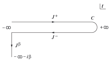
Figure 1: The contour $\mathcal{C}$ in complex time plane in the Schwinger-Keldysh formulation. It consists of a forward branch running from $t=-\infty$ to $t=+\infty$, a backward branch from $t=+\infty$ back to $t=-\infty$, and an imaginary branch from $t=-\infty$ to $t=-\infty-i\beta$. The sources $J^{\pm}$ serve to generate the nonequilibrium Green’s functions of the Nambu-Gor’kov fields.

Since there are three different time evolution operators, the forward, backward and imaginary, we introduce three different sources for each one of these time evolution operators, respectively. Taking $t_{0}\to-\infty$, we are led to considering the generating functional comment

$$Z[J^{+},J^{-},J^{\beta}]=\mathrm{Tr}U(-\infty-i\beta,-\infty,J^{\beta})U(-\infty,+\infty,J^{-})U(+\infty,-\infty;J^{+}),$$ (26)

where $U(t_{f},t_{i};J)$ is the time evolution operator [see (22)] in the presence of the source $J$ and for simplicity of notation we have suppressed the spin index $\sigma$ and the complex conjugate of the sources $J^{\dagger}$. The denominator in (24) is given by $\mathrm{Tr}\rho=Z[0,0,0]$. The generating functional $Z[J^{+},J^{-},J^{\beta}]$ can be written as a path integral along the contour in complex time plane (see Fig. 1)

$$Z[J^{+},J^{-},J^{\beta}]=\int\mathcal{D}_{\mathcal{C}}\Psi^{\dagger}\mathcal{D}_{\mathcal{C}}\Psi\,\exp\left[i\int_{\mathcal{C}}d^{4}x\,\mathcal{L}_{\mathcal{C}}[\Psi^{\dagger},\Psi;J]\right],$$ (27)

where $\mathcal{D}_{\mathcal{C}}\Psi^{\dagger}\mathcal{D}_{\mathcal{C}}\Psi$ denotes the functional integration measure along the contour $\mathcal{C}$ and

$$\int_{\mathcal{C}}d^{4}x\,\mathcal{L}_{\mathcal{C}}[\Psi^{\dagger},\Psi;J] = \int_{-\infty}^{+\infty}d^{4}x\,\mathcal{L}[\Psi^{\dagger+},\Psi^{+};J^{+}]-\int_{-\infty}^{+\infty}d^{4}x\,\mathcal{L}[\Psi^{\dagger-},\Psi^{-};J^{-}]$$ (28)

$$+\,\int_{-\infty}^{-\infty-i\beta}d^{4}x\,\mathcal{L}[\Psi^{\dagger\beta},\Psi^{\beta};J^{\beta}],$$

with $\int_{-\infty}^{+\infty}d^{4}x\equiv\int d^{3}x{}\int_{-\infty}^{+\infty}dt$, etc. Because of the trace and the fermionic nature of the operators, the path integral along the contour $\mathcal{C}$ requires antiperiodic boundary conditions on the fields. The superscripts $+$ and $-$ refer to fields defined in the upper and lower branches, respectively, corresponding to forward ($+$) and backward ($-$) time evolution, while the superscript $\beta$ refers to the field defined in the vertical branch running down parallel to the imaginary axis. The negative sign in front of the action along the backward branch is a result of the fact that backward time evolution is determined by $U^{-1}(+\infty,-\infty)$ with $U$ the time evolution operator. The contour source $J$ that enters in the contour Lagrangian $\mathcal{L}_{\mathcal{C}}$ in (27) takes the values of the sources $J^{\pm}$ and $J^{\beta}$ in the respective branches as displayed in Fig. 1.

Functional derivatives with respect to the sources in the forward branch give time-ordered Green’s functions, those with respect to the sources in the backward branch give the anti-time-ordered Green’s functions, and those with respect to the sources in the imaginary branch give the usual imaginary-time (Matsubara) Green’s functions. While the sources $J^{+}$, $J^{-}$, and $J^{\beta}$ introduced to obtain the Green’s functions via functional differentiation are different in the different branches, as they generate the time-ordered, anti-time-ordered and Matsubara Green’s functions, respectively; the external source $\eta$, the homogeneous condensate $\Delta_{0}$, and the departure from equilibrium $\delta$ are $c$-numbers and hence are the same in all branches.

Writing the Lagrangian as a free and an interaction part as $\mathcal{L}=\mathcal{L}_{0}+\mathcal{L}_{\mathrm{int}}$, the generating functional can be written as a power series expansion in the interaction part, which in turn can be generated by taking functional derivatives with respect to the sources $J$, $J^{\dagger}$ by identifying

$$\Psi^{\pm}\rightarrow\mp i\frac{\delta}{\delta J^{\dagger\pm}},\quad\Psi^{\dagger\pm}\rightarrow\pm i\frac{\delta}{\delta J^{\pm}},$$

$$\Psi^{\beta}\to-i\frac{\delta}{\delta J^{\dagger\beta}},\quad\Psi^{\dagger\beta}\to i\frac{\delta}{\delta J^{\beta}}.$$ (29)

As a result, the full generating functional along the contour $\mathcal{C}$ can be written as

$$Z[J]=\exp\left\{i\int_{\mathcal{C}}d^{4}x\,\mathcal{L}_{\mathrm{int},\mathcal{C}}\left[-i\frac{\delta}{\delta J^{\dagger}},i\frac{\delta}{\delta J}\right]\right\}Z_{0}[J],$$ (30)

where free field generating functional $Z_{0}[J]$ is given by (27) and (28) but with $\mathcal{L}[\Psi^{\dagger},\Psi;J]$ replaced by $\mathcal{L}_{0}[\Psi^{\dagger},\Psi;J]$.

III.2 Green’s functions

The equation of motion for the free Nambu-Gor’kov field $\Psi$ in the presence of the source $J$ reads

$$\left[i\frac{\partial}{\partial t}+\sigma_{3}\left(\frac{\nabla^{2}}{2m}+\mu\right)+\sigma_{+}\Delta_{0}+\sigma_{-}\Delta_{0}^{\ast}\right]\Psi(\mathbf{x}{},t{})=-J(\mathbf{x}{},t{}).$$ (31)

The solution of this equation of motion is given by

$$\Psi_{J}(\mathbf{x}{},t{})=-\int_{\mathcal{C}}d^{4}x^{\prime}S(\mathbf{x}{}-\mathbf{x}{}^{\prime},t-t^{\prime})J(\mathbf{x}{}^{\prime},t^{\prime}),$$ (32)

where $S(\mathbf{x}{}-\mathbf{x}{}^{\prime},t-t^{\prime})$ is the Green’s function matrix along the contour $\mathcal{C}$ and satisfies

$$\left[i\frac{\partial}{\partial t}+\sigma_{3}\left(\frac{\nabla^{2}}{2m}+\mu\right)+\sigma_{+}\Delta_{0}+\sigma_{-}\Delta_{0}^{\ast}\right]S(\mathbf{x}{}-\mathbf{x}{}^{\prime},t-t^{\prime})=\delta_{\mathcal{C}}(t-t^{\prime})\,\delta^{(3)}(\mathbf{x}{}-\mathbf{x}{}^{\prime}),$$ (33)

with $\delta_{\mathcal{C}}(t-t^{\prime})$ the Dirac delta function along the contour $\int_{\mathcal{C}}dt^{\prime}\,\delta_{\mathcal{C}}(t-t^{\prime})=1$. The Green’s function $S(\mathbf{x}{}-\mathbf{x}{}^{\prime},t-t^{\prime})$ has the form

$$S(\mathbf{x}{}-\mathbf{x}{}^{\prime},t-t^{\prime})=S^{>}(\mathbf{x}{}-\mathbf{x}{}^{\prime},t-t^{\prime})\Theta_{\mathcal{C}}(t-t^{\prime})+S^{<}(\mathbf{x}{}-\mathbf{x}{}^{\prime},t-t^{\prime})\Theta_{\mathcal{C}}(t^{\prime}-t),$$ (34)

where $\Theta_{\mathcal{C}}(t-t^{\prime})$ is the step function along the contour and $S^{\gtrless}(\mathbf{x}{}-\mathbf{x}{}^{\prime},t-t^{\prime})$ obey the homogeneous equations of motion.

The antiperiodic boundary conditions on the fields in the path integral, a result of the trace over fermionic fields in (26), lead to the following boundary condition on the Green’s function

$$\lim_{t_{0}\to-\infty}S(\mathbf{x}{}-\mathbf{x}{}^{\prime},t_{0}-t^{\prime})=-\lim_{t_{0}\to-\infty}S(\mathbf{x}{}-\mathbf{x}{}^{\prime},t_{0}-i\beta-t^{\prime}).$$ (35)

Since along the contour $t_{0}\to-\infty$ is the earliest time and $t_{0}-i\beta$ is therefore the latest time, (35) entails

$$\lim_{t_{0}\to-\infty}S^{<}(\mathbf{x}{}-\mathbf{x}{}^{\prime},t_{0}-t^{\prime})=-\lim_{t_{0}\to-\infty}S^{>}(\mathbf{x}{}-\mathbf{x}{}^{\prime},t_{0}-i\beta-t^{\prime}),\quad\forall\;t^{\prime},$$ (36)

which is the Kubo-Martin-Schwinger (KMS) condition for equilibrium correlation functions book:kadanoff .

The free field generating functional $Z_{0}[J]$ is now obtained by writing

$$\Psi(\mathbf{x}{},t)=\widetilde{\Psi}(\mathbf{x}{},t{})+\Psi_{J}(\mathbf{x}{},t{}),$$

$$\Psi^{\dagger}(\mathbf{x}{},t)=\widetilde{\Psi}^{\dagger}(\mathbf{x}{},t{})+\Psi^{\dagger}_{J}(\mathbf{x}{},t{}),$$ (37)

which leads to the result

$$Z_{0}[J]=Z_{0}[0]\exp\left[-i\int_{\mathcal{C}}d^{4}x\int_{\mathcal{C}}d^{4}x^{\prime}J^{\dagger}(x)S(x-x^{\prime})J(x^{\prime})\right],$$ (38)

where and hereafter $x$ denotes the space-time coordinates $(\mathbf{x}{},t{})$ for simplicity of notation. The source independent term $Z_{0}[0]$ will cancel between the numerator and the denominator in all expectation values in (21).

Furthermore, we are interested in computing Green’s functions of finite real times which are defined for fields in the forward ($+$) and backward ($-$) time branches but not in the imaginary branch. For these real-time Green’s functions the contributions to the generating functional from one source in the imaginary branch and another source in either the forward or backward branch vanish by the Riemann-Lebesgue lemma tadpole ; ivp , since the time arguments are infinitely far apart along the contour. Therefore the contour integrals of the source terms and Green’s functions in the generating functional factorize into a term in which the sources are those either in the forward and backward branches and another term in which both sources are in the imaginary branch tadpole ; ivp . The latter term (with both sources in the imaginary branch) cancel between numerator and denominator in expectation values and the only remnant of the imaginary branch is through the periodic boundary conditions along the full contour in the Green’s function.

Thus the generating functional for real-time Green’s functions simplifies to the following expression, defined solely along the forward and backward time branches tadpole ; ivp

$$Z[J^{\pm},J^{\dagger\pm}] = \exp\left[i\int_{-\infty}^{+\infty}d^{4}x\left\{\mathcal{L}_{\mathrm{int}}[-i\delta/\delta J^{\dagger+},i\delta/\delta J^{+}]-\mathcal{L}_{\mathrm{int}}[i\delta/\delta J^{\dagger-},-i\delta/\delta J^{-}]\right\}\right]$$ (39)

$$\times\,\exp\bigg{\{}-i\int_{-\infty}^{+\infty}d^{4}x\int_{-\infty}^{+\infty}d^{4}x^{\prime}\big{[}J^{\dagger+}(x)S^{++}(x-x^{\prime})J^{+}(x^{\prime})+J^{\dagger-}(x)$$

$$\times\,S^{--}(x-x^{\prime})J^{-}(x^{\prime})-J^{\dagger+}(x)S^{+-}(x-x^{\prime})J^{-}(x^{\prime})-J^{\dagger-}(x)S^{-+}(x-x^{\prime})J^{+}(x^{\prime})\big{]}\bigg{\}},$$

with

$$S^{++}(x-x^{\prime})=S^{>}(\mathbf{x}{}-\mathbf{x}{}^{\prime},t-t^{\prime})\Theta(t-t^{\prime})+S^{<}(\mathbf{x}{}-\mathbf{x}{}^{\prime},t-t^{\prime})\Theta(t^{\prime}-t),$$

$$S^{--}(x-x^{\prime})=S^{>}(\mathbf{x}{}-\mathbf{x}{}^{\prime},t-t^{\prime})\Theta(t^{\prime}-t)+S^{<}(\mathbf{x}{}-\mathbf{x}{}^{\prime},t-t^{\prime})\Theta(t-t^{\prime}),$$

$$S^{-+}(x-x^{\prime})=S^{>}(\mathbf{x}{}-\mathbf{x}{}^{\prime},t-t^{\prime}),$$

$$S^{+-}(x-x^{\prime})=S^{<}(\mathbf{x}{}-\mathbf{x}{}^{\prime},t-t^{\prime}),$$ (40)

where now $-\infty\leq t,t^{\prime}\leq+\infty$ and the superscripts $+$, $-$ correspond to the sources defined on the forward ($+$) and backward ($-$) time branches, respectively. An important issue that must be highlighted at this stage, is that derivatives with respect to sources in the forward ($+$) time branch correspond to insertion of operators pre-multiplying the density matrix $\rho$ and derivatives with respect to sources in the backward ($-$) branch correspond to the insertion of operators post-multiplying the density matrix. That this is so is a consequence of the fact that the density matrix evolves in time as $U(t,t_{0})\rho_{0}U^{-1}(t,t_{0})$ with $U(t,t_{0})$ the time evolution operator.

These four Green’s functions are not independent because of the identity

$$S^{++}(x-x^{\prime})+S^{--}(x-x^{\prime})-S^{+-}(x-x^{\prime})-S^{-+}(x-x^{\prime})=0.$$ (41)

The diagonal elements in $S^{++}(x-x^{\prime})$ are the normal Green’s functions, representing the propagation of single electrons, whereas the off-diagonal elements are the anomalous Green’s functions, corresponding to the annihilation and creation of two electrons of opposite spins, respectively.

The functions $S^{\gtrless}(x-x^{\prime})$, which are solutions of the homogeneous free field equation of motion, are simply related to the correlation functions of the free Nambu-Gor’kov fields $\Psi$, $\Psi^{\dagger}$. Indeed, taking variational derivatives of the free field generating functional $Z_{0}[J]$ with respect to $J^{\pm}$, $J^{\dagger\pm}$, one can show that

$$S^{>}_{ab}(x-x^{\prime})=-i\langle\Psi_{a}(x)\Psi_{b}^{\dagger}(x^{\prime})\rangle,$$

$$S^{<}_{ab}(x-x^{\prime})=i\langle\Psi_{b}^{\dagger}(x^{\prime})\Psi_{a}(x)\rangle,$$ (42)

where and hereafter $a,b=1,2$ denote the Nambu-Gor’kov indices. The expectation values in the expressions above are in the non-interacting thermal density matrix which corresponds to the quadratic part of the Lagrangian (Hamiltonian), i.e., the density matrix that describes free Bogoliubov quasiparticles in thermal equilibrium at inverse temperature $\beta$.

While the matrix elements $S^{\gtrless}_{ab}(x-x^{\prime})$ can be obtained through the usual Bogoliubov transformation to the quasiparticle basis book:fetter , we present in the Appendix an alternative derivation of these correlation functions directly from the spinor solutions of the homogeneous equations of motion. We find that the correlation functions in (42) in the infinite volume limit are given by

$$S^{\gtrless}_{ab}(x-x^{\prime})=\int\frac{d^{3}k}{(2\pi)^{3}}S^{\gtrless}_{ab}(k,t-t^{\prime})\,e^{i\mathbf{k}\cdot(\mathbf{x}{}-\mathbf{x}{}^{\prime})},$$ (43)

where

$$S^{>}_{ab}(k,t-t^{\prime})=-i\left[[1-n_{\mathrm{F}}(E_{k})]\,\mathcal{S}_{ab}(k)\,e^{-iE_{k}(t-t^{\prime})}+n_{\mathrm{F}}(E_{k})\,\overline{\mathcal{S}}_{ab}(k)\,e^{iE_{k}(t-t^{\prime})}\right],$$

$$S^{<}_{ab}(k,t-t^{\prime})=i\left[n_{\mathrm{F}}(E_{k})\,\mathcal{S}_{ab}(k)\,e^{-iE_{k}(t-t^{\prime})}+[1-n_{\mathrm{F}}(E_{k})]\,\overline{\mathcal{S}}_{ab}(k)\,e^{iE_{k}(t-t^{\prime})}\right],$$ (44)

with

$$\mathcal{S}(k)=\begin{bmatrix}u^{2}_{k}&-u_{k}v_{k}^{\ast}\\ -u_{k}v_{k}&|v_{k}|^{2}\end{bmatrix},\quad\overline{\mathcal{S}}(k)=\begin{bmatrix}|v_{k}|^{2}&u_{k}v_{k}^{\ast}\\ u_{k}v_{k}&u^{2}_{k}\end{bmatrix}.$$ (45)

In the above expressions $k\equiv|\mathbf{k}|$, $n_{\mathrm{F}}(\omega)=1/(e^{\beta\omega}+1)$ is the Fermi-Dirac distribution function, $u_{k}$ and $v_{k}$ satisfying $u_{k}^{2}+|v_{k}|^{2}=1$ are the Bogoliubov coefficients [see (145)], and $E_{k}$ is the energy of free Bogoliubov quasiparticles (bogolons)

$$E_{k}=\sqrt{\xi_{k}^{2}+|\Delta_{0}|^{2}},$$ (46)

where $\xi_{k}=k^{2}/2m-\mu$ (see the Appendix). Using the relation $1-n_{\mathrm{F}}(\omega)=e^{\beta\omega}\,n_{\mathrm{F}}(\omega)$, one can easily verify the KMS condition book:kadanoff

$$S^{>}(k,t-i\beta-t^{\prime})=-S^{<}(k,t-t^{\prime}).$$ (47)

Hence, the correlation functions for the Nambu-Gor’kov fields $\Psi$, $\Psi^{\dagger}$ that will enter in the nonequilibrium perturbative expansion are completely determined by (42)-(46).

III.3 Feynman rules

From the generating functional of nonequilibrium Green’s functions (39), it is clear that the effective interaction Lagrangian relevant for the nonequilibrium calculations is given by

$$\mathcal{L}_{\mathrm{int}}^{\mathrm{eff}}[\Psi^{\dagger\pm},\Psi^{\pm},\chi^{\dagger\pm},\chi^{\pm}]=\mathcal{L}_{\mathrm{int}}[\Psi^{\dagger+},\Psi^{+},\chi^{\dagger+},\chi^{+}]-\mathcal{L}_{\mathrm{int}}[\Psi^{\dagger-},\Psi^{-},\chi^{\dagger-},\chi^{-}],$$ (48)

where the fields $\Psi^{\dagger\pm}$, $\Psi^{\pm}$, $\chi^{\dagger\pm}$ and $\chi^{\pm}$ are defined on the forward ($+$) and backwards ($-$) time branches respectively. Consequently, this generating functional leads to the following Feynman rules that define the perturbative expansion for calculations of nonequilibrium expectation values.

• There are two sets of interaction vertices defined by $\mathcal{L}_{\mathrm{int}}^{\mathrm{eff}}[\Psi^{\dagger\pm},\Psi^{\pm},\chi^{\dagger\pm},\chi^{\pm}]$: those in which the fields are in the forward ($+$) branch and those in which the fields are in the backward ($-$) branch. There is a relative minus sign between these two types of vertices.

• For each kind of fields there are four types of Green’s functions corresponding to correlations between fields defined in the forward or backward branch.

  The Green’s functions of the Nambu-Gor’kov fields $\Psi$, $\Psi^{\dagger}$ are given by (40) in terms of the correlation functions displayed in (42) that are completely determined by (44), (45) and (46).

  The Green’s functions of the pair fields $\chi$, $\chi^{\dagger}$ can be obtained in an analogous manner. However, due to the nonpropagating nature of the pair fields, the Green’s functions are local in time and hence those of fields defined in different branches vanish identically.

• The combinatoric factors, trace over the Nambu-Gor’kov indices for fermion loops, etc., are the same as in the imaginary-time (Matsubara) formulation.

IV Relaxation of condensate perturbations: An initial value problem

IV.1 Equations of motion

The equations of motion for the small amplitude superconducting condensate perturbation $\delta(x)$ induced by the external source $\eta(x)$ is obtained by implementing the tadpole method tadpole ; ivp . This method begins by writing the pair fields $\Delta^{\pm}(x)$ in the forward ($+$) and backward ($-$) time branches as

$$\Delta^{\pm}(x)=\Delta_{0}+\delta(x)+\chi^{\pm}(x),$$ (49)

where $\Delta_{0}$ is the homogeneous condensate in the absence of external source, $\delta(x)$ is the perturbation of the condensate induced by the external source which vanishes in the absence of external source, and $\chi^{\pm}(x)$ are the noncondensate part of the pair fields in the forward and backward time branches. The external source $\eta(x)$ are $c$-number fields and hence taken the same value in both forward and backward branches. The strategy to obtain the equations of motion for small amplitude condensate perturbation $\delta(x)$, $\delta^{\ast}(x)$ is to consider the interaction Lagrangian $\mathcal{L}_{\mathrm{int}}[\Psi^{\dagger},\Psi,\chi^{\dagger},\chi]$ given in (20) in perturbation theory and impose the tadpole condition

$$\langle\chi^{\pm}(x)\rangle_{\eta}=\langle\chi^{\dagger\pm}(x)\rangle_{\eta}=0$$ (50)

order by order in the perturbative expansion, but, consistent with linear response, only keep contributions linear in $\delta(x)$, $\delta^{\ast}(x)$.

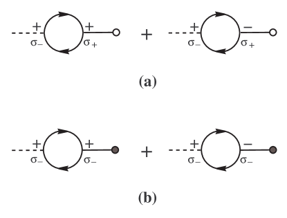
Figure 2: Feynman diagrams contributing to the retarded self-energies (a) $\Sigma_{11}(x-x^{\prime})$ and (b) $\Sigma_{12}(x-x^{\prime})$ to one-loop order. A solid line with arrow denotes the Nambu-Gor’kov field, a dashed line denotes the pair field, and a solid line with open (filled) circle denotes the condensate perturbation $\delta$ ($\delta^{\ast}$).

Using the Feynman rules described in the previous section, to one-loop order the tadpole condition $\langle\chi^{+}(0)\rangle_{\eta}=\langle\chi^{\dagger+}(0)\rangle_{\eta}=0$ leads to the following expression

$$\int d^{4}x\langle\chi^{+}(0)\chi^{\dagger+}(x)\rangle\bigg{[}\frac{\delta(x)}{g}+\int d^{4}x^{\prime}\big{[}\Sigma_{11}(x-x^{\prime})\delta(x^{\prime})+\Sigma_{12}(x-x^{\prime})\delta^{\ast}(x^{\prime})\big{]}+\mathcal{T}(\Delta_{0},\Delta^{\ast}_{0})-\eta(x)\bigg{]}=0,$$

$$\int d^{4}x\langle\chi^{\dagger+}(0)\chi^{+}(x)\rangle\bigg{[}\frac{\delta^{\ast}(x)}{g}+\int d^{4}x^{\prime}\big{[}\Sigma_{22}(x-x^{\prime})\delta^{\ast}(x^{\prime})+\Sigma_{21}(x-x^{\prime})\delta(x^{\prime})\big{]}+\mathcal{T}^{\ast}(\Delta_{0},\Delta^{\ast}_{0})-\eta^{\ast}(x)\bigg{]}=0,$$ (51)

where $\Sigma_{ab}(x-x^{\prime})$ are the retarded self-energies of the pair fields and the tadpole $\mathcal{T}(\Delta_{0},\Delta^{\ast}_{0})$ denotes terms independent of the condensate perturbation $\delta$, $\delta^{\ast}$. The diagrams for $\Sigma_{11}(x-x^{\prime})$ and $\Sigma_{12}(x-x^{\prime})$ to one-loop order are depicted in Fig. 2, and those for $\Sigma_{22}(x-x^{\prime})$ and $\Sigma_{21}(x-x^{\prime})$ can be obtained in an analogous manner. Explicitly to one-loop order we find

$$\Sigma_{11}(x-x^{\prime}) = -i\left[\langle\Psi^{\dagger+}(x)\sigma_{-}\Psi^{+}(x)\Psi^{\dagger+}(x^{\prime})\sigma_{+}\Psi^{+}(x^{\prime})\rangle-\langle\Psi^{\dagger+}(x)\sigma_{-}\Psi^{+}(x)\Psi^{\dagger-}(x^{\prime})\sigma_{+}\Psi^{-}(x^{\prime})\rangle\right]$$

$$= -i\,\textrm{tr}\left[\sigma_{-}S^{++}(x-x^{\prime})\sigma_{+}S^{++}(x^{\prime}-x)-\sigma_{-}S^{+-}(x-x^{\prime})\sigma_{+}S^{-+}(x^{\prime}-x)\right],$$

$$\Sigma_{12}(x-x^{\prime}) = -i\left[\langle\Psi^{\dagger+}(x)\sigma_{-}\Psi^{+}(x)\Psi^{\dagger+}(x^{\prime})\sigma_{-}\Psi^{+}(x^{\prime})\rangle-\langle\Psi^{\dagger+}(x)\sigma_{-}\Psi^{+}(x)\Psi^{\dagger-}(x^{\prime})\sigma_{-}\Psi^{-}(x^{\prime})\rangle\right]$$ (52)

$$= -i\,\textrm{tr}\left[\sigma_{-}S^{++}(x-x^{\prime})\sigma_{-}S^{++}(x^{\prime}-x)-\sigma_{-}S^{+-}(x-x^{\prime})\sigma_{-}S^{-+}(x^{\prime}-x)\right],$$

where $\mathrm{tr}$ denotes the trace over the Nambu-Gor’kov indices. The expressions for $\Sigma_{22}(x-x^{\prime})$ and $\Sigma_{21}(x-x^{\prime})$ can be obtained, respectively, from expressions in (52) through the replacement $\sigma_{+}\leftrightarrow\sigma_{-}$.

The diagrams for the tadpole $\mathcal{T}(\Delta_{0},\Delta^{\ast}_{0})$ are depicted in Fig. 3, from which we find

$$\mathcal{T}(\Delta_{0},\Delta^{\ast}_{0}) = \frac{\Delta_{0}}{g}-\langle\Psi^{\dagger+}(x)\sigma_{-}\Psi^{+}(x)\rangle$$ (53)

$$= \frac{\Delta_{0}}{g}+i\,\mathrm{tr}\left[\sigma_{-}S^{<}(0)\right].$$

A simple calculation with the nonequilibrium Green’s functions of the Nambu-Gor’kov fields obtained in the previous section shows that the tadpole to one-loop order is given by

$$\mathcal{T}(\Delta_{0},\Delta^{\ast}_{0})=\Delta_{0}\left[\frac{1}{g}-\int\frac{d^{3}q}{(2\pi)^{3}}\frac{1-2n_{\mathrm{F}}(E_{q})}{2E_{q}}\right],$$ (54)

where $E_{q}$ on the right-hand side of (54) is understood to be a function of $|\Delta_{0}|$ [see (46)] and, hereafter, the momentum integral $\int\frac{d^{3}q}{(2\pi)^{3}}$ is restricted to the electronic states near the Fermi surface.

It is customary to rewrite the integral over the momentum $\mathbf{q}$ as being over the energy $\xi$ (measured from the Fermi surface) at the expense of introducing the density of states $\mathcal{N}(\xi)$, which is taken to be constant near the Fermi surface, and cutting the integral off at $\pm\omega_{\mathrm{D}}$ with $\omega_{\mathrm{D}}$ being the Debye energy, thus leading to

$$\mathcal{T}(\Delta_{0},\Delta^{\ast}_{0})=\Delta_{0}\left[\frac{1}{g}-\mathcal{N}(0)\int_{0}^{\omega_{\mathrm{D}}}\frac{d\xi}{E}\,[1-2n_{\mathrm{F}}(E)]\right],$$ (55)

where $E=\sqrt{\xi^{2}+|\Delta_{0}|^{2}}$ and $\mathcal{N}(0)=mk_{\mathrm{F}}/2\pi^{2}$ is the density of states at the Fermi surface. Setting the external source $\eta=0$, the equilibrium condition for the homogeneous condensate $\mathcal{T}(\Delta_{0},\Delta^{\ast}_{0})=0$ becomes

$$\Delta_{0}\left[\frac{1}{g}-\mathcal{N}(0)\int_{0}^{\omega_{\mathrm{D}}}\frac{d\xi}{E}\,[1-2n_{\mathrm{F}}(E)]\right]=0.$$ (56)

In equilibrium and below the critical temperature, the condensate $\Delta_{0}\neq 0$. Therefore (56) leads to the finite-temperature BCS gap equation that determines $\Delta_{0}(T)$:

$$g\mathcal{N}(0)\int_{0}^{\omega_{\mathrm{D}}}\frac{d\xi}{E}\,[1-2n_{\mathrm{F}}(E)]=1.$$ (57)

Introducing the space Fourier transforms for $\delta(x)$, $\eta(x)$ and $\Sigma_{ab}(x-x^{\prime})$ as

$$\delta(\mathbf{x}{},t{})=\int\frac{d^{3}k}{(2\pi)^{3}}\,\delta_{\mathbf{k}}(t)\,e^{i\mathbf{k}\cdot\mathbf{x}{}},$$

etc., we find the equations of motion in momentum space to be given by

$$\delta_{\mathbf{k}}(t)+g\int_{-\infty}^{+\infty}dt^{\prime}\left[\Sigma_{11}(\mathbf{k},t-t^{\prime})\,\delta_{\mathbf{k}}(t^{\prime})+\Sigma_{12}(\mathbf{k},t-t^{\prime})\,\delta^{\ast}_{-\mathbf{k}}(t^{\prime})\right]+g\mathcal{T}(\Delta_{0},\Delta^{\ast}_{0})\,\delta^{(3)}(\mathbf{k})-g\eta_{\mathbf{k}}(t)=0,$$

$$\delta^{\ast}_{-\mathbf{k}}(t)+g\int_{-\infty}^{+\infty}dt^{\prime}\left[\Sigma_{22}(\mathbf{k},t-t^{\prime})\,\delta^{\ast}_{-\mathbf{k}}(t^{\prime})+\Sigma_{21}(\mathbf{k},t-t^{\prime})\,\delta_{\mathbf{k}}(t^{\prime})\right]+g\mathcal{T}^{\ast}(\Delta_{0},\Delta^{\ast}_{0})\,\delta^{(3)}(\mathbf{k})-g\eta^{\ast}_{-\mathbf{k}}(t)=0.$$ (58)

The equations of motion obtained from the tadpole condition $\langle\chi^{-}(0)\rangle_{\eta}=\langle\chi^{\dagger-}(0)\rangle_{\eta}=0$ are the same as those given in the above expressions. While the equations of motion (58) are obtained to one-loop order, it is straightforward to conclude after a simple diagrammatic analysis that the structure of the equations of motion obtained above is general and valid to all orders in perturbation theory.

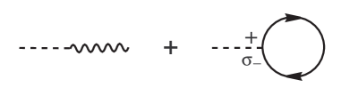
Figure 3: Feynman diagrams contributing to the tadpole $\mathcal{T}(\Delta_{0},\Delta^{\ast}_{0})$ to one-loop order. A wiggly line denotes the homogeneous condensate $\Delta_{0}$.

From the explicit expressions for the self-energies or by taking complex conjugation of the equation of motion for $\delta_{\mathbf{k}}(t)$, one can show that

$$\Sigma_{21}(\mathbf{k},t-t^{\prime})=\Sigma^{\ast}_{12}(-\mathbf{k},t-t^{\prime}),$$

$$\Sigma_{22}(\mathbf{k},t-t^{\prime})=\Sigma^{\ast}_{11}(-\mathbf{k},t-t^{\prime}).$$ (59)

Furthermore, rotational and parity invariance imply that the self-energies are only functions of $k$. Upon expressing the nonequilibrium Green’s functions in terms of the correlation functions $S^{\gtrless}$, one finds immediately that the retarded self-energies have the following causal structure

$$\Sigma_{11}(\mathbf{k},t-t^{\prime})=\Sigma^{R}_{11}(k,t-t^{\prime})\,\Theta(t-t^{\prime}),$$

$$\Sigma_{12}(\mathbf{k},t-t^{\prime})=\Sigma^{R}_{12}(k,t-t^{\prime})\,\Theta(t-t^{\prime}).$$ (60)

Before proceeding further, we note that the invariance of the Lagrangian under the global gauge transformation (16) implies that all the terms in the equations of motion for $\delta$ ($\delta^{\ast}$) must transform as $\delta$ ($\delta^{\ast}$) itself under the gauge transformation. This in turn entails that the normal self-energies $\Sigma_{11}$ and $\Sigma_{22}$ must be invariant under the gauge transformation (16), while the anomalous ones $\Sigma_{12}$ and $\Sigma_{21}$ must transform as $\Delta^{2}_{0}$ and $\Delta^{\ast 2}_{0}$, respectively. Thus, it is proves convenient to write

$$\Sigma^{R}_{11}(k,t-t^{\prime})=\Sigma^{R\ast}_{22}(k,t-t^{\prime})=\Sigma_{D}(k,t-t^{\prime}),$$

$$\Sigma^{R}_{12}(k,t-t^{\prime})=\Sigma^{R\ast}_{21}(k,t-t^{\prime})=(\Delta_{0}/\Delta_{0}^{\ast})\Sigma_{O}(k,t-t^{\prime}),$$ (61)

where both $\Sigma_{D}$ and$\Sigma_{O}$ are invariant under the gauge transformation (16). While rewriting the self-energies in this manner may seem a redundant exercise, the main point is to highlight and make explicit their transformation laws under the gauge transformation. This is an important aspect that needs to be addressed carefully in order to extract the Ward identities, an exact result of the underlying gauge symmetry to be explored below.

The gauge invariant self-energies $\Sigma_{D}$ and $\Sigma_{O}$ can be written in terms of their spectral representation as

$$\Sigma_{D}(k,t-t^{\prime})=\int^{+\infty}_{-\infty}d\omega\left[\overline{A}(k,\omega)\sin\omega(t-t^{\prime})+i\overline{S}(k,\omega)\cos\omega(t-t^{\prime})\right],$$

$$\Sigma_{O}(k,t-t^{\prime})=\int^{+\infty}_{-\infty}d\omega\,\widehat{A}(k,\omega)\sin\omega(t-t^{\prime}).$$ (62)

The symmetric ($\overline{S}$) and antisymmetric ($\overline{A}$, $\widehat{A}$) spectral functions are, respectively, even and odd functions of $\omega$ and are to be given by

$$\overline{S}(k,\omega) = -\frac{1}{4}\int\frac{d^{3}q}{(2\pi)^{3}}\bigg{\{}[1-n_{\mathrm{F}}(E_{q})-n_{\mathrm{F}}(E_{p})]\left(\frac{\xi_{q}}{E_{q}}+\frac{\xi_{p}}{E_{p}}\right)[\delta(\omega-E_{q}-E_{p})+\delta(\omega+E_{q}+E_{p})]$$

$$-\,[n_{\mathrm{F}}(E_{q})-n_{\mathrm{F}}(E_{p})]\left(\frac{\xi_{q}}{E_{q}}-\frac{\xi_{p}}{E_{p}}\right)[\delta(\omega-E_{q}+E_{p})+\delta(\omega+E_{q}-E_{p})]\bigg{\}},$$

$$\overline{A}(k,\omega) = -\frac{1}{4}\int\frac{d^{3}q}{(2\pi)^{3}}\bigg{\{}[1-n_{\mathrm{F}}(E_{q})-n_{\mathrm{F}}(E_{p})]\left(1+\frac{\xi_{q}\xi_{p}}{E_{q}E_{p}}\right)[\delta(\omega-E_{q}-E_{p})-\delta(\omega+E_{q}+E_{p})]$$

$$-\,[n_{\mathrm{F}}(E_{q})-n_{\mathrm{F}}(E_{p})]\left(1-\frac{\xi_{q}\xi_{p}}{E_{q}E_{p}}\right)[\delta(\omega-E_{q}+E_{p})-\delta(\omega+E_{q}-E_{p})]\bigg{\}},$$

$$\widehat{A}(k,\omega) = \frac{1}{4}\int\frac{d^{3}q}{(2\pi)^{3}}\frac{|\Delta_{0}|^{2}}{E_{q}E_{p}}\Big{\{}[1-n_{\mathrm{F}}(E_{q})-n_{\mathrm{F}}(E_{p})][\delta(\omega-E_{q}-E_{p})-\delta(\omega+E_{q}+E_{p})]$$ (63)

$$+\,[n_{\mathrm{F}}(E_{q})-n_{\mathrm{F}}(E_{p})][\delta(\omega-E_{q}+E_{p})-\delta(\omega+E_{q}-E_{p})]\Big{\}},$$

where $p=|\mathbf{k}+\mathbf{q}|$ and $\xi_{q}=q^{2}/2m-\mu$.

The terms proportional to $[1-n_{\mathrm{F}}(E_{q})-n_{\mathrm{F}}(E_{p})]$ in the above expressions correspond to processes in which two quasiparticles are either created or destroyed, whereas the terms proportional to $[n_{\mathrm{F}}(E_{q})-n_{\mathrm{F}}(E_{p})]$ arise from Landau damping processes corresponding to scattering of quasiparticle excitations in the medium.

In an experimental situation the dynamical evolution of the small amplitude condensate perturbation is studied by preparing a superconducting state slightly perturbed away from equilibrium by adiabatically coupling to some external source in the infinite past. Once the source is switched-off at time $t=0$ the perturbed condensate relaxes towards equilibrium and the relaxation dynamics is studied. As discussed above, this experimental situation can be realized within the real-time formulation described here by taking the spatial Fourier transform of the external source to be of the form

$$\eta_{\mathbf{k}}(t)=\eta_{\mathbf{k}}\,e^{\epsilon t}\,\Theta(-t),\quad\epsilon\to 0^{+}.$$ (64)

The $\epsilon$-term serves to switch on the source adiabatically from $t=-\infty$ so as not to disturb the system too far from equilibrium in the process. If at $t=-\infty$ the system was in an equilibrium state, then the condition of equilibrium (56) ensures that for $t<0$ there is a solution of the equations of motion (58) of the form

$$\delta_{\mathbf{k}}(t)=\delta_{\mathbf{k}}(0)\,e^{\epsilon t}\quad\mathrm{for}\;\;t<0,$$ (65)

where $\delta_{\mathbf{k}}(0)$ is related to $\eta_{\mathbf{k}}$ through the equations of motion for $t<0$. The advantage of the adiabatic switching-on of the external source is that the time derivative of the solution (65) satisfies $\dot{\delta}_{\mathbf{k}}(t<0)\to 0$ as $\epsilon\to 0^{+}$.

Let us introduce auxiliary quantities $\Pi^{R}_{ab}(k,t-t^{\prime})$ defined as

$$\Sigma^{R}_{ab}(k,t-t^{\prime})=\partial_{t^{\prime}}\Pi^{R}_{ab}(k,t-t^{\prime}),$$ (66)

then upon using integration by parts, neglecting terms that vanish in the adiabatic limit $\epsilon\to 0^{+}$, and taking $\Delta_{0}$ to be the equilibrium condensate and hence $\mathcal{T}(\Delta_{0},\Delta^{\ast}_{0})=0$, we find the equations of motion (58) become

$$[1+g\Pi^{R}_{11}(k,0)]\delta_{\mathbf{k}}(t)+g\Pi^{R}_{12}(k,0)\delta^{\ast}_{-\mathbf{k}}(t)-g\int_{0}^{t}dt^{\prime}\big{[}\Pi^{R}_{11}(k,t-t^{\prime})\dot{\delta}_{\mathbf{k}}(t^{\prime})+\Pi^{R}_{12}(k,t-t^{\prime})\dot{\delta}^{\ast}_{-\mathbf{k}}(t^{\prime})\big{]}=0,$$

$$[1+g\Pi^{R}_{22}(k,0)]\delta^{\ast}_{-\mathbf{k}}(t)+g\Pi^{R}_{21}(k,0)\delta_{\mathbf{k}}(t)-g\int_{0}^{t}dt^{\prime}\big{[}\Pi^{R}_{22}(k,t-t^{\prime})\dot{\delta}^{\ast}_{-\mathbf{k}}(t^{\prime})+\Pi^{R}_{21}(k,t-t^{\prime})\dot{\delta}_{\mathbf{k}}(t^{\prime})\big{]}=0.$$ (67)

The above coupled equations of motion for the condensate perturbation are now in the form of an initial value problem with initial conditions specified at $t=0$ and can be solved by Laplace transform. Introducing a two-component Nambu-Gor’kov spinor and its Laplace transform

$$\phi_{\mathbf{k}}(t)=\begin{bmatrix}\delta_{\mathbf{k}}(t)\\ \delta^{\ast}_{-\mathbf{k}}(t)\end{bmatrix},\quad\widetilde{\phi}_{\mathbf{k}}(s)=\begin{bmatrix}\widetilde{\delta}_{\mathbf{k}}(s)\\ \widetilde{\delta}^{\ast}_{-\mathbf{k}}(s)\end{bmatrix},$$ (68)

where $s$ is the Laplace variable, one can rewrite the Laplace transformed equations of motion in a compact matrix form as

$$\widetilde{G}^{-1}(k,s)\,\widetilde{\phi}_{\mathbf{k}}(s)=\frac{1}{s}\big{[}\widetilde{G}^{-1}(k,s)-\widetilde{G}^{-1}(k,0)\big{]}\phi_{\mathbf{k}}(0).$$ (69)

In the above equation, $\widetilde{G}^{-1}(k,s)$ is the inverse Green’s function (matrix) to one-loop order expressed in terms of the Laplace variable $s$

$$\widetilde{G}^{-1}(k,s)=\begin{bmatrix}1+g\widetilde{\Sigma}_{D}(k,s)&g(\Delta_{0}/\Delta_{0}^{\ast})\widetilde{\Sigma}_{O}(k,s)\\ g(\Delta_{0}^{\ast}/\Delta_{0})\widetilde{\Sigma}_{O}(k,s)&1+g\widetilde{\Sigma}_{D}(k,-s)\end{bmatrix},$$ (70)

where $\widetilde{\Sigma}_{D}$ and $\widetilde{\Sigma}_{O}$ are the Laplace transforms of $\Sigma_{D}$ and $\Sigma_{O}$, respectively,

$$\widetilde{\Sigma}_{D}(k,s)=\int^{+\infty}_{-\infty}\frac{dk_{0}}{k_{0}-is}\,\left[\overline{A}(k,k_{0})+\overline{S}(k,k_{0})\right],$$

$$\widetilde{\Sigma}_{O}(k,s)=\int^{+\infty}_{-\infty}\frac{dk_{0}}{k_{0}-is}\widehat{A}(k,k_{0}).$$ (71)

The solution of (70) reads

$$\widetilde{\phi}_{\mathbf{k}}(s)=\frac{1}{s}\,[1-\widetilde{G}(k,s)\,\widetilde{G}^{-1}(k,0)]\,\phi_{\mathbf{k}}(0),$$ (72)

where

$$\widetilde{G}(k,s)=\frac{1}{\widetilde{D}(k,s)}\begin{bmatrix}1+g\widetilde{\Sigma}_{D}(k,-s)&-g(\Delta_{0}/\Delta_{0}^{\ast})\widetilde{\Sigma}_{O}(k,s)\\ -g(\Delta_{0}^{\ast}/\Delta_{0})\widetilde{\Sigma}_{O}(k,s)&1+g\widetilde{\Sigma}_{D}(k,s)\end{bmatrix},$$ (73)

with the denominator $\widetilde{D}(k,s)$ given by

$$\widetilde{D}(k,s)=[1+g\widetilde{\Sigma}_{D}(k,s)][1+g\widetilde{\Sigma}_{D}(k,-s)]-[g\widetilde{\Sigma}_{O}(k,s)]^{2}.$$ (74)

The real-time evolution of the condensate perturbation $\phi_{\mathbf{k}}(t)$ with an initial value $\phi_{\mathbf{k}}(0)$ is now obtained from the inverse Laplace transform

$$\phi_{\mathbf{k}}(t)=\int_{\mathcal{B}}\frac{ds}{2\pi i}\,e^{st}\,\widetilde{\phi}_{\mathbf{k}}(s),$$ (75)

where the Bromwich contour $\mathcal{B}$ runs parallel to the imaginary axis in the complex $s$ plane to the right of all the singularities (poles and cuts) of $\widetilde{\phi}_{\mathbf{k}}(s)$ ivp . We note that there is no isolated pole in $\widetilde{\phi}_{\mathbf{k}}(s)$ at $s=0$ since the residue vanishes.

IV.2 Self-energies in the long-wavelength, low-frequency limit

In this article we are interested to study the relaxation of long-wavelength, low-frequency fluctuations of the pair field, hence our next task is to expand the self-energies as a function of $k,\,s$ up to $\mathcal{O}(k^{2},s^{2})$. With $\xi_{q}=q^{2}/2m-\mu$ and $p=|\mathbf{q}+\mathbf{k}|$ we use the following approximations

$$\xi_{p}\approx\xi_{q}+\delta\xi,\quad\delta\xi=v_{\mathrm{F}}k\cos\theta,$$

$$E_{p}=E_{q}+\xi_{q}\frac{\delta\xi}{E_{q}}+\frac{(\delta\xi)^{2}}{2}\frac{|\Delta_{0}|^{2}}{E^{3}_{q}},$$ (76)

where $\theta$ is the angle between $\widehat{\mathbf{k}}$ and $\widehat{\mathbf{q}}$. We keep only up to terms of $\mathcal{O}(k^{2},s^{2})$ in the Laplace transform of the self-energies and obtain

$$\widetilde{\Sigma}_{D}(k,s) = -\mathcal{N}(0)\int^{\omega_{\mathrm{D}}}_{0}d\xi\bigg{\{}\frac{1-2n_{\mathrm{F}}(E)}{2E}\bigg{[}\bigg{(}1+\frac{\xi^{2}}{E^{2}}\bigg{)}\left(1-\frac{v_{\mathrm{F}}^{2}k^{2}}{12E^{2}}-\frac{s^{2}}{4E^{2}}\right)-\left(3-\frac{5\xi^{2}}{E^{2}}\right)\frac{v_{\mathrm{F}}^{2}k^{2}\xi^{2}}{6E^{4}}\bigg{]}$$

$$-\,\frac{\partial n_{\mathrm{F}}(E)}{\partial E}\frac{|\Delta_{0}|^{2}}{E^{2}}\bigg{[}\frac{v_{\mathrm{F}}^{2}k^{2}\xi^{2}}{2E^{4}}+\left(1-\frac{3s^{2}}{2E^{2}}\right)\bigg{(}1-\frac{isE}{2v_{\mathrm{F}}k\xi}\ln\frac{is/v_{\mathrm{F}}k+\xi/E}{is/v_{\mathrm{F}}k-\xi/E}\bigg{)}\bigg{]}\bigg{\}}+\cdots,$$

$$\widetilde{\Sigma}_{O}(k,s) = \mathcal{N}(0)\int^{\omega_{\mathrm{D}}}_{0}d\xi\frac{|\Delta_{0}|^{2}}{E^{2}}\bigg{\{}\frac{1-2n_{\mathrm{F}}(E)}{2E}\bigg{[}1-\left(\frac{1}{4}-\frac{5\xi^{2}}{6E^{2}}\right)\frac{v_{\mathrm{F}}^{2}k^{2}}{E^{2}}-\frac{s^{2}}{4E^{2}}\bigg{]}$$ (77)

$$-\,\frac{\partial n_{\mathrm{F}}(E)}{\partial E}\bigg{[}\frac{v_{\mathrm{F}}^{2}k^{2}}{2E^{2}}\left(\frac{1}{3}-\frac{\xi^{2}}{E^{2}}\right)-\left(1-\frac{3s^{2}}{2E^{2}}+\frac{s^{2}}{\xi^{2}}\right)\bigg{(}1-\frac{isE}{2v_{\mathrm{F}}k\xi}\ln\frac{is/v_{\mathrm{F}}k+\xi/E}{is/v_{\mathrm{F}}k-\xi/E}\bigg{)}\bigg{]}\bigg{\}}+\cdots,$$

where $E=\sqrt{\xi^{2}+|\Delta_{0}|^{2}}$ and the dots stand for terms of higher order in the ratios $k/|\Delta_{0}|,s/|\Delta_{0}|$. We note that to this order both $\widetilde{\Sigma}_{D}(k,s)$ and $\widetilde{\Sigma}_{O}(k,s)$ are even functions of the Laplace variable $s$. This important feature leads to the decoupling of the phase and amplitude fluctuations of the pair field in the equations of motion, as will be shown below.

IV.3 One-loop effective action

The full equations of motion in real time (58) and their Laplace transform around the equilibrium state (69) allow us to obtain at once the retarded effective action in Fourier space. The retarded Green’s function kernel is obtained from $\widetilde{G}^{-1}(k,s)$ in (69) by the analytic continuation in the complex $s$ plane $s\to-i\omega+0^{+}$. In terms of the Fourier transform (retarded) of the two-component Nambu-Gor’kov spinor and the tadpole spinor

$$\mathcal{T}_{\mathbf{k}}(\omega)=\begin{bmatrix}\mathcal{T}(\Delta_{0},\Delta^{\ast}_{0})\\ \mathcal{T}^{\ast}(\Delta_{0},\Delta^{\ast}_{0})\end{bmatrix}\delta^{(3)}(\mathbf{k})\delta(\omega),$$ (78)

the retarded one-loop effective action to quadratic order in the fluctuations is therefore given by

$$S[\delta,\delta^{\ast}]=S[0,0]+\frac{1}{2g}\int d^{3}kd\omega\left[\phi^{\dagger}_{-\mathbf{k}}(-\omega)G^{-1}(k,\omega)\phi_{\mathbf{k}}(\omega)+2\phi^{\dagger}_{-\mathbf{k}}(-\omega)\mathcal{T}_{\mathbf{k}}(\omega)\right],$$ (79)

where $G^{-1}(k,\omega)=\widetilde{G}^{-1}(k,s=-i\omega+0^{+})$ and $S[0,0]$ is a function of $\Delta_{0}$, $\Delta^{\ast}_{0}$ such that

$$\frac{\partial S[0,0]}{\partial\Delta^{\ast}_{0}}=\mathcal{T}(\Delta_{0},\Delta^{\ast}_{0}),\quad\frac{\partial S[0,0]}{\partial\Delta_{0}}=\mathcal{T}^{\ast}(\Delta_{0},\Delta^{\ast}_{0}).$$ (80)

Obviously, variational derivatives with respect to $\delta,\,\delta^{\ast}$ reproduce the retarded equations of motion. We identify (79) with the one-loop effective action quadratic in the fluctuations.

V Ward identity and static self-energies

The Ward identities, a consequence of the underlying (global) gauge invariance, are an integral part of the program to establish a connection with the Ginzburg-Landau description. Furthermore the equations of motion must fulfill these for consistency. In this section we show how the Ward identities emerge directly from the method described above used to obtain the equations of motion.

A straightforward diagrammatic analysis with the Feynman rules described above reveals that the generic structure of the equations of motion obtained via the tadpole method remains the same to all orders in perturbation theory. When combined with the transformation properties of $\Delta_{0}$, $\delta$ and $\chi$ under the gauge transformation (16), this general form of the equations of motion allows to derive to all orders in perturbation theory the Ward identity for the tadpole $\mathcal{T}(\Delta_{0},\Delta^{\ast}_{0})$.

First, consider the case in which $\delta,\,\eta=0$ the tadpole condition $\langle\chi^{+}(0)\rangle_{\eta}=0$ leads to $\mathcal{T}(\Delta_{0},\Delta^{\ast}_{0})=0$, which is the equilibrium condition for the homogeneous condensate. For a space-time independent shift of the condensate $\Delta_{0}\to\Delta_{0}+\delta$ induced by a space-time independent source $\eta$, the tadpole condition now leads to $\mathcal{T}(\Delta_{0}+\delta,\Delta_{0}^{\ast}+\delta^{\ast})=-\eta$, which upon expanding to linear order in $\delta$ and $\delta^{\ast}$ becomes

$$\mathcal{T}(\Delta_{0},\Delta^{\ast}_{0})+\frac{\partial\mathcal{T}(\Delta_{0},\Delta^{\ast}_{0})}{\partial\Delta_{0}}\,\delta+\frac{\partial\mathcal{T}(\Delta_{0},\Delta^{\ast}_{0})}{\partial\Delta_{0}^{\ast}}\,\delta^{\ast}=-\eta.$$ (81)

We now compare (81) with the first equation of motion given in (58), which has the same generic structure as the full equation of motion obtained to all orders in perturbation theory, for space-time independent $\delta$ and $\delta^{\ast}$. Comparing the coefficients of $\delta,\delta^{\ast}$ we recognize immediately that

$$\frac{\partial\mathcal{T}(\Delta_{0},\Delta^{\ast}_{0})}{\partial\Delta_{0}} = \frac{1}{g}+\Sigma_{11}(k=0,\omega=0),$$

$$\frac{\partial\mathcal{T}(\Delta_{0},\Delta^{\ast}_{0})}{\partial\Delta_{0}^{\ast}} = \Sigma_{12}(k=0,\omega=0),$$ (82)

which relate the self-energies at zero frequency and zero momentum to the derivatives of the tadpole with respect to the condensate and is valid to all orders in perturbation theory.

The second important ingredient and which stems from the equations of motion (58) is that under a global gauge (phase) transformation (16) the tadpole $\mathcal{T}(\Delta_{0},\Delta^{\ast}_{0})$ transforms just as $\delta$, $\Delta_{0}$ and $\eta$, i.e., $\mathcal{T}(e^{i\theta}\Delta_{0},e^{-i\theta}\Delta_{0}^{\ast})=e^{i\theta}\mathcal{T}(\Delta_{0},\Delta^{\ast}_{0})$. Taking the gauge parameter $\theta$ to be infinitesimal and comparing the linear terms in $\theta$, we find to all orders in perturbation theory the Ward identity for the tadpole

$$\mathcal{T}(\Delta_{0},\Delta^{\ast}_{0})=\frac{\partial\mathcal{T}(\Delta_{0},\Delta^{\ast}_{0})}{\partial\Delta_{0}}~{}\Delta_{0}-\frac{\partial\mathcal{T}(\Delta_{0},\Delta^{\ast}_{0})}{\partial\Delta_{0}^{\ast}}\Delta_{0}^{\ast}.$$ (83)

Therefore upon combining (82) and the Ward identity (83), we obtain an alternative statement of the Ward identity which is an exact relationship between the tadpole and the self-energies at zero frequency and momentum

$$\Delta_{0}\left[\frac{1}{g}+\Sigma_{11}(0,0)\right]-\Delta_{0}^{\ast}\,\Sigma_{12}(0,0)=\mathcal{T}(\Delta_{0},\Delta^{\ast}_{0}),$$ (84)

where $\Sigma_{ab}(0,0)$ stands for $\Sigma_{ab}(k=0,\omega=0)$ for notational simplicity. Above the critical temperature, both the tadpole and the condensate vanish thus the above equation becomes a trivial identity. However, below the critical temperature $\Delta_{0}\neq 0$ and hence (84) leads to

$$\frac{g\mathcal{T}(\Delta_{0},\Delta^{\ast}_{0})}{\Delta_{0}}=1+g\left[\Sigma_{11}(0,0)-\frac{\Delta_{0}^{\ast}}{\Delta_{0}}\Sigma_{12}(0,0)\right].$$ (85)

It is customary to choose the condensate to be real by redefining its phase via the gauge transformation (16). However, as argued above, for a condensate with an arbitrary phase, the anomalous self-energy $\Sigma_{12}$ must be proportional to $\Delta_{0}^{2}$ since in the equation of motion it multiplies $\delta^{\ast}$, which transforms under gauge transformations just as $\Delta_{0}^{\ast}$. This fact can be seen explicitly at the one-loop order in the expressions for the respective anomalous self-energy in (61) as well as in (62) with the spectral functions given by (63). Since the product $\Sigma_{12}\delta^{\ast}$ must transform just as $\delta$ or $\Delta_{0}$, therefore the phase $\Delta_{0}^{\ast}/\Delta_{0}$ cancels the phase of $\Delta^{2}_{0}$ in $\Sigma_{12}$. In terms of the gauge invariant self-energies $\Sigma_{D}$ and $\Sigma_{O}$, the Ward identity (85) can be cast into an explicit gauge invariant form

$$\frac{g\mathcal{T}(\Delta_{0},\Delta^{\ast}_{0})}{\Delta_{0}}=1+g\Sigma_{D}(0,0)-g\Sigma_{O}(0,0).$$ (86)

We emphasize that the Ward identity (85) or (86) is an exact relationship valid in or out of equilibrium (corresponding to when the tadpole $\mathcal{T}(\Delta_{0},\Delta^{\ast}_{0})$ vanishes or not, respectively). In equilibrium the equilibrium condition $\mathcal{T}(\Delta_{0},\Delta^{\ast}_{0})=0$ implies that the self-energies in the static limit must satisfy the relation

$$1+g\Sigma_{D}(0,0)-g\Sigma_{O}(0,0)=0.$$ (87)

The long-wavelength limit of the static self-energies is defined as

$$\Sigma_{D}(0,0)=\lim_{k\to 0}\lim_{s\to 0}\Sigma_{D}(k,s),$$

$$\Sigma_{O}(0,0)=\lim_{k\to 0}\lim_{s\to 0}\Sigma_{O}(k,s),$$ (88)

which, using (77), are found to one-loop order given by

$$\Sigma_{D}(0,0)=-\mathcal{N}(0)\int_{0}^{\omega_{\mathrm{D}}}d\xi\,\bigg{[}\frac{1-2n_{\mathrm{F}}(E)}{2E}\left(1+\frac{\xi^{2}}{E^{2}}\right)-\frac{\partial n_{\mathrm{F}}(E)}{\partial E}\frac{|\Delta_{0}|^{2}}{E^{2}}\bigg{]},$$

$$\Sigma_{O}(0,0)=\mathcal{N}(0)\int_{0}^{\omega_{\mathrm{D}}}d\xi\,\frac{|\Delta_{0}|^{2}}{E^{2}}\bigg{[}\frac{1-2n_{\mathrm{F}}(E)}{2E}+\frac{\partial n_{\mathrm{F}}(E)}{\partial E}\bigg{]}.$$ (89)

The opposite limit $\lim_{s\to 0}\lim_{k\to 0}\Sigma_{D,O}(k,s)$ yields the first terms in the expressions (89) but not the last terms proportional to $\partial n_{\mathrm{F}}(E)/\partial E$. This is a consequence of the non-analyticity of the Landau damping contributions to the self-energies.

Using the expression for the one-loop tadpole given by (55) it becomes clear that the identities (82) are fulfilled by the precise order of limits determined by (89), i.e., the long-wavelength limit of the static ($s=0$) self-energies.

We now show explicitly that the Ward identity (86) is fulfilled to one-loop order. The tadpole to one-loop order is given by (55). From the explicit form of the one-loop self-energies in the static limit (89), find that

$$\Sigma_{D}(0,0)-\Sigma_{O}(0,0)=-\mathcal{N}(0)\int_{0}^{\omega_{\mathrm{D}}}\frac{d\xi}{E}\,[1-2n_{\mathrm{F}}(E)],$$ (90)

which is an exact relationship to one-loop order, obtained for arbitrary $\Delta_{0}$.

Upon collecting the above results, we find to one-loop order that

$$\frac{g\mathcal{T}(\Delta_{0},\Delta^{\ast}_{0})}{\Delta_{0}} = 1+g\Sigma_{D}(0,0)-g\Sigma_{O}(0,0)$$ (91)

$$= 1-g\mathcal{N}(0)\int_{0}^{\omega_{\mathrm{D}}}\frac{d\xi}{E}\,[1-2n_{\mathrm{F}}(E)].$$

Therefore, the Ward identity (86) is manifestly fulfilled to one-loop order. This is an important advantage of the tadpole method of nonequilibrium field theory: the equations of motion obtained at a given order in the loop expansion are causal and guaranteed to fulfill the corresponding Ward identities to that order.

We highlight that whereas the Ward identity is independent of the limits, $k,s\to 0$, the individual self-energies have different limits because of the non-analyticity of the Landau damping contribution. The relationship between the self-energies and the tadpole (82) is only valid in the static limit (89).

The results of this section, namely the Ward identity which relates the self-energies to derivatives of the tadpole will play an important role in the derivation of the effective Ginzburg-Landau theory.

VI Time-dependent Ginzburg-Landau Theory

We are now in position to establish contact with the Ginzburg-Landau description of the long-wavelength, low-frequency excitations near the critical point. The Ginzburg-Landau description in terms of a functional of the order parameter is valid near the critical region when $|T-T_{c}|\ll T_{c},\Delta(T)\simeq\left[T_{c}(T_{c}-T)\right]^{1/2}\ll T_{c}$. The link between the Ginzburg-Landau (GL) theory and the microscopic theory of superconductivity in the static limit was established by Gor’kov gorkov59 .

Identifying the expectation value of the pair field $\Delta\equiv\langle\Delta(\mathbf{x}{},t{})\rangle$ as the complex order parameter, the free energy in Ginzburg-Landau theory for an homogeneous order parameter (absence of gradients) is given by

$$\mathcal{F}(\Delta,\Delta^{\ast})=a(T)|\Delta|^{2}+\frac{b}{2}|\Delta|^{4},$$ (92)

where near the critical temperature $a(T)\propto(T-T_{c})$.

The linearized equation of motion of the small amplitude fluctuation of the condensate can be obtained by expanding the free energy around the equilibrium value of gap function; namely $\Delta_{0}$ and $\Delta_{0}^{\ast}$. Writing $\Delta=\Delta_{0}+\delta$ and $\Delta^{\ast}=\Delta_{0}^{\ast}+\delta^{\ast}$, keeping only quadratic terms in the fluctuations:

$$\mathcal{F}(\Delta,\Delta^{\ast})=\mathcal{F}(\Delta_{0},\Delta^{\ast}_{0})+\delta\frac{\partial\mathcal{F}}{\partial\Delta}+\delta^{\ast}\frac{\partial\mathcal{F}}{\partial\Delta^{\ast}}+\delta\delta^{\ast}\frac{\partial^{2}\mathcal{F}}{\partial\Delta\partial\Delta^{\ast}}+\frac{\delta^{2}}{2}\frac{\partial^{2}\mathcal{F}}{\partial\Delta^{2}}+\frac{\delta^{\ast 2}}{2}\frac{\partial^{2}\mathcal{F}}{\partial\Delta^{\ast 2}}.$$ (93)

The linearized equation of motion for both $\delta$ and $\delta^{\ast}$ can then be obtained by minimizing $\mathcal{F}$ with respect to $\delta^{\ast}$ and $\delta$ respectively and are given by

$$\Sigma^{\mathrm{GL}}_{11}\,\delta+\Sigma^{\mathrm{GL}}_{12}\delta^{\ast}+{\mathcal{T}}^{\mathrm{GL}}(\Delta_{0},\Delta^{\ast}_{0})=0,$$

$$\Sigma^{\mathrm{GL}}_{22}\delta^{\ast}+\Sigma^{\mathrm{GL}}_{21}\delta+[{\mathcal{T}}^{\mathrm{GL}}(\Delta_{0},\Delta^{\ast}_{0})]^{\ast}=0,$$ (94)

with

$${\mathcal{T}}^{\mathrm{GL}}(\Delta_{0},\Delta^{\ast}_{0})=\Delta_{0}\left[a(T)+b|\Delta_{0}|^{2}\right],$$

$$\Sigma^{\mathrm{GL}}_{11}=[\Sigma^{\mathrm{GL}}_{22}]^{\ast}=a(T)+2b|\Delta_{0}|^{2}\equiv\frac{\partial{\mathcal{T}}^{\mathrm{GL}}}{\partial\Delta_{0}},$$

$$\Sigma^{\mathrm{GL}}_{12}=[\Sigma^{\mathrm{GL}}_{21}]^{\ast}=b\Delta^{2}_{0}\equiv\frac{\partial{\mathcal{T}}^{\mathrm{GL}}}{\partial\Delta^{\ast}_{0}}.$$ (95)

The gap equation obtained from the Ginzburg-Landau free energy (92) is

$${\mathcal{T}}^{\mathrm{GL}}(\Delta_{0},\Delta^{\ast}_{0})=0,$$ (96)

which determines the equilibrium value of the order parameter for $\delta=\delta^{\ast}=0$. When the gap equation (96) is fulfilled, the matrix of the second derivatives of the free energy (92) with respect to $\delta,\delta^{\ast}$ has a zero eigenvalue with eigenvector determined by the relation

$$\delta^{\ast}=-\frac{\Delta^{\ast}_{0}}{\Delta_{0}}\delta.$$ (97)

Obviously this eigenvector with zero eigenvalue corresponds to a phase fluctuation and is the Goldstone boson, or the Anderson-Bogoliubov-Goldstone mode, associated with the broken global gauge symmetry.

The similarity between the equations of motion (94) and (58) for an homogeneous perturbation with vanishing external sources, as well as the similarities between the identities (95) and (82), (84) are now obvious and suggest the following identification

$$\mathcal{T}(\Delta_{0},\Delta^{\ast}_{0}) \Longleftrightarrow \mathcal{T}^{\mathrm{GL}}(\Delta_{0},\Delta^{\ast}_{0}),$$

$$\frac{1}{g}+\Sigma_{11}(0,0) \Longleftrightarrow \Sigma^{\mathrm{GL}}_{11},$$

$$\Sigma_{12}(0,0) \Longleftrightarrow \Sigma^{\mathrm{GL}}_{12},$$ (98)

where the self-energies on the left-hand side of the relations are understood as the long-wavelength limit of the static self energies as discussed in Sec. V. This similarity can be put on firmer footing by expanding the one-loop expression for the tadpole $\mathcal{T}(\Delta_{0},\Delta^{\ast}_{0})$ (55) in terms of a power series expansion in $\Delta_{0},\Delta^{\ast}_{0}$ and keeping up to third order consistently with the Ginzburg-Landau expansion.

Using the form of the tadpole given in (55) and the results obtained in Ref. ketterson, , we find ($\hbar=k_{\mathrm{B}}=1$)

$$g\mathcal{T}(\Delta_{0},\Delta^{\ast}_{0})=\left[1-g\mathcal{N}(0)\ln\left(\frac{1.14\omega_{\mathrm{D}}}{T}\right)\right]\Delta_{0}+\frac{7g\mathcal{N}(0)\zeta(3)}{8\pi^{2}T^{2}_{c}}\Delta_{0}|\Delta_{0}|^{2}+\mathcal{O}(\Delta_{0}^{5}),$$ (99)

where $\zeta$ is the Riemann zeta function with $\zeta(3)=1.202$ and $T_{c}=1.14\,\omega_{\mathrm{D}}\,e^{-1/g\mathcal{N}(0)}$. For $T\approx T_{c}$ the coefficient of the linear term can be expanded as $g\mathcal{N}(0)(T-T_{c})/T_{c}$, therefore from the relations (82) and the definitions (61) we obtain

$$1+g\Sigma_{D}(0,0) = g\mathcal{N}(0)\left(\frac{T-T_{c}}{T_{c}}\right)+\frac{7g\mathcal{N}(0)\zeta(3)}{4\pi^{2}T^{2}_{c}}|\Delta_{0}|^{2},$$

$$g\Sigma_{O}(0,0) = \frac{7g\mathcal{N}(0)\zeta(3)}{8\pi^{2}T^{2}_{c}}|\Delta_{0}|^{2}.$$ (100)

We now focus on the long-wavelength, low-frequency self-energies in the Ginzburg-Landau regime characterized by $v_{\mathrm{F}}k,s\ll|\Delta_{0}|\ll T$. This regime corresponds to the description of the long-wavelength, low-frequency excitations near the critical point and will allow a consistent analysis of the real-time dynamics of (small) phase and amplitude fluctuations. We begin by writing the long-wavelength, low-frequency self-energies as [see (77)]

$$\widetilde{\Sigma}_{D}(k,s) = \Sigma_{D}(0,0)+I(k,s),$$

$$\widetilde{\Sigma}_{O}(k,s) = \Sigma_{O}(0,0)+J(k,s),$$ (101)

with $\Sigma_{D,O}(0,0)$ given by (89). Since the self-energies are dimensionless functions of their arguments, the expansion in terms of $k$ and $s$ must involve ratios of these variables and the typical scales in the integrals. There are two, widely separated scales in the Ginzburg-Landau regime, namely, $T\approx T_{c}$ and $|\Delta_{0}|$ with $|\Delta_{0}|/T\ll 1$. The expressions for $I,J$ feature energy denominators that would lead to infrared divergences if $|\Delta_{0}|$ is set to zero. These divergences reflect the presence of inverse powers of $|\Delta_{0}|$ in the expansions.

The leading terms in the expansion can be extracted by rescaling

$$\xi=|\Delta_{0}|z,\quad E=|\Delta_{0}|\epsilon,$$ (102)

with $\epsilon=\sqrt{z^{2}+1}$ and introducing the dimensionless variables

$$x=\frac{|\Delta_{0}|}{T},\quad\kappa=\frac{v_{\mathrm{F}}k}{|\Delta_{0}|},\quad\bar{s}=\frac{s}{v_{\mathrm{F}}k},$$ (103)

in the integrals for $I(k,s)$ and $J(k,s)$. We obtain

$$I(k,s)=\mathcal{N}(0)\,x\left[\kappa^{2}I_{a}(x)+\kappa^{2}\bar{s}^{2}I_{b}(\bar{s},x)+i\bar{s}I_{c}(\bar{s},x)\right],$$ (104)

where

$$I_{a}(x) = \frac{1}{4}\int^{\infty}_{0}dz\left\{\frac{2T(x,z)}{3x\epsilon^{3}}\left[\frac{2z^{2}}{\epsilon^{4}}-\frac{z^{2}-1}{4\epsilon^{2}}\left(1+\frac{z^{2}}{\epsilon^{2}}\right)\right]-\frac{C(x,z)z^{2}}{2\epsilon^{6}})\right\},$$

$$I_{b}\left(\bar{s},x\right) = \frac{1}{4}\int^{\infty}_{0}dz\left\{\frac{T(x,z)}{2x\epsilon^{3}}\left(1+\frac{z^{2}}{\epsilon^{2}}\right)+\frac{3C(x,z)}{2\epsilon^{4}}\left[1-\frac{i\bar{s}\epsilon}{2z}\ln\frac{i\bar{s}+z/\epsilon}{i\bar{s}-z/\epsilon}\right]\right\},$$

$$I_{c}\left(\bar{s},x\right) = \frac{1}{4}\int^{\infty}_{0}dz\left[\frac{C(x,z)}{2z\epsilon}\ln\frac{i\bar{s}+z/\epsilon}{i\bar{s}-z/\epsilon}\right],$$ (105)

with

$$T(x,z)=\tanh\left(\frac{x\epsilon}{2}\right),\quad C(x,z)=\cosh^{-2}\left(\frac{x\epsilon}{2}\right).$$ (106)

Similarly, for $J(k,s)$ we obtain

$$J(k,s)=\mathcal{N}(0)\,x\left[\kappa^{2}J_{a}(x)+\kappa^{2}\bar{s}^{2}J_{b}(\bar{s},x)+i\bar{s}J_{c}(\bar{s},x)\right],$$ (107)

where

$$J_{a}(x) = \frac{1}{24}\int^{\infty}_{0}dz\left[T(x,z)\frac{7z^{2}-3}{x\epsilon^{7}}-C(x,z)\frac{2z^{2}-1}{\epsilon^{6}}\right],$$

$$J_{b}\left(\bar{s},x\right) = -\frac{1}{8}\int^{\infty}_{0}dz\left\{\frac{T(x,z)}{x\epsilon^{5}}-C(x,z)\frac{2z^{2}-1}{z^{2}\epsilon^{4}}\left[1-\frac{i\bar{s}\epsilon}{2z}\ln\frac{i\bar{s}+z/\epsilon}{i\bar{s}-z/\epsilon}\right]\right\},$$

$$J_{c}\left(\bar{s},x\right) = I_{c}\left(\bar{s},x\right).$$ (108)

An important consequence of the long-wavelength, low-frequency expansion of the self-energies in (101) together with (105), (108) is that to lowest order the self-energies are even functions of the Laplace variable $s$. This important aspect leads to the decoupling of the phase and amplitude fluctuations in the equations of motion, as can be seen as follows.

If we write the fluctuation of the order parameter around the space-time constant equilibrium solution of the tadpole equation (56) in the form

$$\Delta(x,t) = \Delta_{0}+\delta(x,t)$$ (109)

$$\equiv [\rho_{0}+\delta\rho(x,t)]\,e^{i\theta_{0}+i\delta\theta(x,t)},$$

where $\delta\rho(x,t)$ and $\delta\theta(x,t)$, respectively, are identified as the amplitude and phase fluctuations of the order parameter $\Delta(x,t)$. It is convenient to introduce the following projection vectors

$$\mathbf{p} = \frac{1}{\sqrt{2}i}\begin{bmatrix}1\\ -\frac{\Delta^{\ast}_{0}}{\Delta_{0}}\end{bmatrix},\quad\mathbf{p}^{\dagger}=-\frac{1}{\sqrt{2}i}\left[1,-\frac{\Delta_{0}}{\Delta^{\ast}_{0}}\right],$$

$$\mathbf{a} = \frac{1}{\sqrt{2}}\begin{bmatrix}1\\ \frac{\Delta^{\ast}_{0}}{\Delta_{0}}\end{bmatrix},\quad\mathbf{a}^{\dagger}=\frac{1}{\sqrt{2}}\left[1,\frac{\Delta_{0}}{\Delta^{\ast}_{0}}\right],$$ (110)

in terms of these vectors and the Nambu-Gor’kov spinors (68), the phase and amplitude fluctuations can be written as

$$\delta\theta(x,t)=\frac{1}{\sqrt{2}\Delta_{0}}\mathbf{p}^{\dagger}\cdot\phi(x,t),\quad\frac{\delta\rho(x,t)}{\rho_{0}}=\frac{1}{\sqrt{2}\Delta_{0}}\mathbf{a}^{\dagger}\cdot\phi(x,t),$$ (111)

or, equivalently,

$$\widetilde{\phi}_{\mathbf{k}}(s)=\sqrt{2}\Delta_{0}\left[\widetilde{\delta\theta}_{\mathbf{k}}(s)\mathbf{p}+\frac{\widetilde{\delta\rho}_{\mathbf{k}}(s)}{\rho_{0}}\mathbf{a}\right].$$ (112)

In terms of the Laplace transforms $\widetilde{\delta\theta}_{\mathbf{k}}(s)$ and $\widetilde{\delta\rho}_{\mathbf{k}}(s)$, the equations of motion (69) now become

$$\left[1+g\widetilde{\Sigma}_{D}(k,s)-g\widetilde{\Sigma}_{O}(k,s)\right]\widetilde{\delta\theta}_{\mathbf{k}}(s)=\frac{g}{s}\left[\left(\widetilde{\Sigma}_{D}(k,s)-\widetilde{\Sigma}_{O}(k,s)\right)-\left(\widetilde{\Sigma}_{D}(k,0)-\widetilde{\Sigma}_{O}(k,0)\right)\right]\delta\theta_{\mathbf{k}}(0),$$

$$\left[1+g\widetilde{\Sigma}_{D}(k,s)+g\widetilde{\Sigma}_{O}(k,s)\right]\widetilde{\delta\rho}_{\mathbf{k}}(s)=\frac{g}{s}\left[\left(\widetilde{\Sigma}_{D}(k,s)+\widetilde{\Sigma}_{O}(k,s)\right)-\left(\widetilde{\Sigma}_{D}(k,0)+\widetilde{\Sigma}_{O}(k,0)\right)\right]\delta\rho_{\mathbf{k}}(0).$$ (113)

The decoupling of the equations of motion between phase and amplitude fluctuations is a direct consequence of the fact that self-energies are even functions of the Laplace variable to this, lowest order. In particular the equality $\Sigma_{D}(k,s)=\Sigma_{D}(k,-s)$ to this order guarantees that the vectors $\mathbf{p}$ and $\mathbf{a}$ are eigenvectors of the matrix $\widetilde{G}^{-1}(k,s)$ in (69). The right-hand sides of (VI) are identified as the Laplace transform of the source terms $J_{\theta}$, $J_{\rho}$, respectively, that serve the purpose of setting up the initial value problem.

In particular to lowest order in the long-wavelength expansion, and after the analytic continuation $s\to-i\omega+0^{+}$, the retarded one-loop effective action for fluctuations around the equilibrium solution is given, up to a constant, by

$$S_{\mathrm{eff}}\left[\delta\theta,\delta\rho\right] = \frac{|\Delta_{0}|^{2}}{2g}\int d^{3}kd\omega\left\{\delta\theta_{-\mathbf{k}}(-\omega)\left[1+g\Sigma_{D}(k,\omega)-g\Sigma_{O}(k,\omega)\right]\delta\theta_{\mathbf{k}}(\omega)+2J_{\theta,-\mathbf{k}}(-\omega)\delta\theta_{\mathbf{k}}(\omega)\right\}$$ (114)

$$+\,\frac{1}{2g}\int d^{3}kd\omega\left\{\delta\rho_{-\mathbf{k}}(-\omega)\left[1+g\Sigma_{D}(k,\omega)+g\Sigma_{O}(k,\omega)\right]\delta\rho_{\mathbf{k}}(\omega)+2J_{\rho,-\mathbf{k}}(-\omega)\delta\rho_{\mathbf{k}}(\omega)\right\},$$

where $\Sigma_{D,O}(k,\omega)=\widetilde{\Sigma}_{D,O}(k,s=-i\omega+0^{+})$ and the momentum integral must be understood to be restricted near the Fermi surface. Expanding the self-energies as in (101) together with (105), (108) and using the Ward identities (86) valid in equilibrium, one can easily show that the phase fluctuations are Goldstone modes. Using the explicit expressions for $I(k,s)$ and $J(k,s)$, we find that the effective action for the phase fluctuation is identical to that obtained in Refs. aitchison97, ; aitchison95, to quadratic order, while the effective action for the amplitude fluctuation is a new contribution.

The approach followed here, based directly on the equations of motion in real time also allows us to obtain the effective action for the amplitude fluctuations on the same footing.

VI.1 Phase fluctuations

The initial value problem for the phase and amplitude fluctuations described by the equations of motions (VI) can now be studied straightforwardly. For the phase fluctuation the inverse Laplace transform is obtained by integrating $\widetilde{\delta\theta}_{\mathbf{k}}(s)$ along the Bromwich contour in the complex $s$ plane parallel to the imaginary axis and to the right of all the singularities of the Laplace transform

$$\frac{\widetilde{\delta\theta}_{\mathbf{k}}(s)}{{\delta\theta}_{\mathbf{k}}(0)}=\frac{1}{s}\frac{F(\bar{s},x)}{F(\bar{s},x)+f(x)},$$ (115)

where

$$f(x)=I_{a}(x)-J_{a}(x),$$

$$F(\bar{s},x)=\bar{s}^{2}\left[I_{b}\left(\bar{s},x\right)-J_{b}\left(\bar{s},x\right)\right].$$ (116)

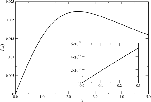
Figure 4: The full $x$ dependence of $f(x)$ is plotted for $0<x<5$. The inset shows $f(x)$ in the Ginzburg-Landau regime $x\ll 1$.

In the Ginzburg-Landau regime $x\ll 1$, we find from (105) and (108) that

$$f(x) \simeq -\frac{x}{12}\int^{\infty}_{0}\frac{dz}{z^{3}}\left[\tanh\frac{z}{2}-\frac{z}{2}\right]+\mathcal{O}(x^{2})$$ (117)

$$= \frac{7\zeta(3)}{48\pi^{2}}x+\mathcal{O}(x^{2}).$$

Figure 4 displays a numerical evaluation of $f(x)$ with the full $x$ dependence. It shows clearly that $f(x)\ll 1$ and that $f(x)$ is accurately described by (117) in the Ginzburg-Landau regime.

To leading order in $x$, we can set $x\to 0$ in the arguments when evaluating $F(\bar{s},x)$. After the analytic continuation $s\to-i\omega+0^{+}$ and introducing the dimensionless variable

$$\alpha=\frac{\omega}{v_{\mathrm{F}}k},$$ (118)

we find in the Ginzburg-Landau regime that the real and imaginary parts of $F(\bar{s}=-i\alpha+0^{+},0)$ are, respectively, given by (here we have set $x\to 0$)

$$F_{\mathrm{R}}(\alpha) = \frac{\alpha^{2}}{8}\int^{\infty}_{0}\frac{dz}{\epsilon^{2}}\left[1+\frac{1}{z^{2}}\left(1-\frac{\alpha\epsilon}{2z}\ln\left|\frac{\alpha+\frac{z}{\epsilon}}{\alpha-\frac{z}{\epsilon}}\right|\right)\right]$$

$$\stackrel{{\scriptstyle\alpha\ll 1}}{{\simeq}} \frac{\pi^{2}|\alpha|^{3}}{64},$$

$$F_{\mathrm{I}}(\alpha) = \frac{\pi\alpha^{3}}{16}\Theta(1-\alpha^{2})\int^{\infty}_{z_{\mathrm{min}}}\frac{dz}{z^{3}\epsilon}$$ (119)

$$\stackrel{{\scriptstyle\alpha\ll 1}}{{\simeq}} \frac{\pi\alpha}{32},$$

where $z_{\mathrm{min}}=\sqrt{\alpha^{2}/(1-\alpha^{2})}$ and we have set $x\to 0$ in the argument of $F(\bar{s},x)$. These expressions agree with those found by Aitchison et al. aitchison97 in the limit $x\to 0$ comparison1 .

The real [$F_{\mathrm{R}}(\alpha)$] and imaginary [$F_{\mathrm{I}}(\alpha)$] parts of $F(\alpha)$ for $0\leq\alpha\leq 1$ are displayed in Fig. 5. The real part is a monotonically increasing function of $\alpha$ while the imaginary part only has contribution in the Landau damping cut $-1<\alpha<1$ corresponding to $-v_{\mathrm{F}}k<\omega<v_{\mathrm{F}}k$.

Figure 5: Real and imaginary parts of $F(\alpha)$.

Isolated real poles of the Laplace transform, describing stable quasiparticle excitations, correspond to the solutions of the following equations

$$F_{\mathrm{R}}(\alpha)-f(x)=0,\quad F_{\mathrm{I}}(\alpha)=0.$$ (120)

It is clear from (117) and Fig. 5 that the first equation in (120) can be fulfilled for $f(x)\ll 1$ only in a region where $F_{\mathrm{I}}(\alpha)\neq 0$. Therefore in the Ginzburg-Landau regime the long-wavelength, low-frequency Laplace transform (115) has no isolated quasiparticle poles, the only singularity is a branch cut in the imaginary axis $-iv_{\mathrm{F}}k<s<iv_{\mathrm{F}}k$, a consequence of Landau damping.

Having understood the analytic structure of the Laplace transform, we can now proceed to study the time evolution via the inverse Laplace transform (75) by closing the Bromwich contour wrapping around the cut $-iv_{\mathrm{F}}k<s<iv_{\mathrm{F}}k$. We obtain

$$\delta\theta_{\mathbf{k}}(t)=\int^{1}_{-1}\frac{d\alpha}{\alpha}\,\rho_{\mathrm{ph}}(\alpha)\cos(\alpha\tau)\,\delta\theta_{\mathbf{k}}(0),$$ (121)

where $\tau=v_{\mathrm{F}}kt$ and the spectral density for the phase fluctuations is given by

$$\rho_{\mathrm{ph}}(\alpha)=\frac{1}{\pi}\frac{f(x)F_{\mathrm{I}}(\alpha)}{\left[F_{\mathrm{R}}(\alpha)-f(x)\right]^{2}+F_{\mathrm{I}}^{2}(\alpha)}.$$ (122)

Figure 6: Spectral density $\rho_{\mathrm{ph}}(\alpha)$ vs $\alpha$ in the Ginzburg-Landau regime.

The spectral density $\rho_{\mathrm{ph}}(\alpha)$ and the real-time evolution of $\delta\theta_{\mathbf{k}}(t)$ for several values of $x\lesssim 1$ are displayed in Figs. 6 and 7, respectively. Three important features are gleaned from these figures:

• The spectral density features a sharp peak at a value $\alpha_{\mathrm{peak}}(x)$ that vanishes continuously as $x\to 0$. This peak would indicate quasiparticle excitations with dispersion relation $\omega=\alpha_{\mathrm{peak}}(x)v_{\mathrm{F}}k$. The group velocity $v_{\mathrm{g}}(x)\simeq 14\,\zeta(3)v_{\mathrm{F}}x/3\pi^{3}$ vanishes at the critical point $x=0$ and increases linearly with $x$ at least within the range $0<x\lesssim 0.2$.

• While the spectral density is not of the Breit-Wigner type (Lorentzian or resonance) and hence a true width cannot be extracted unambiguously, it is clear from the figure that qualitatively the quasiparticle excitations have a “width”. This width vanishes at the critical point and increases monotonically with $x\ll 1$ at least within the range consistent with a Ginzburg-Landau expansion. Therefore these quasiparticles will be Landau damped below $T_{c}$ and the relaxation time scale (the inverse of the “width”) diverges at the critical point $x=0$. This expectation will be confirmed below and suggests critical slowing down of long-wavelength phase fluctuations.

• The reason that despite the appearance of a sharp peak in the spectral density near the critical point the real-time dynamics does not reveal the oscillations associated with a “quasiparticle pole” is clear. As $x\to 0$ both the damping rate and the group velocity $v_{\mathrm{g}}(x)$ vanish in such a way that the time scale for damping is either shorter or of the same order as the time scale for the oscillation.

Furthermore, (121) evaluated at $t=0$ leads to the sum rule

$$\int^{1}_{-1}\frac{d\alpha}{\alpha}\,\rho_{\mathrm{ph}}(\alpha)=1,$$ (123)

which we have confirmed numerically for a wide range of $x$.

It is clear that damping becomes more pronounced for larger $x$ and while the peak would seem to lead to oscillations with period $2\pi/\alpha_{\mathrm{peak}}(x)$ there are no hints of oscillatory behavior in the real-time evolution. Phase fluctuations are strongly overdamped without featuring a propagating mode. Hence we conclude that near the critical point, in the Ginzburg-Landau regime $x\ll 1$, Goldstone modes or phase fluctuations are severely damped despite the fact that the spectral density features a peak that would indicate a quasiparticle “dispersion relation” $\omega=\alpha_{\mathrm{peak}}(x)k$. The damping becomes larger for larger $x$ and is solely a consequence of collisionless Landau damping.

Figure 7: Real-time evolution of the phase fluctuation $\delta\theta_{\mathbf{k}}(\tau)$ vs $\tau$ in the Ginzburg-Landau regime is plotted in linear scale (top) and logarithmic scale (bottom).

For $x\ll 1$, we find that the nonequilibrium relaxation of the phase fluctuation is very well approximated by an exponential (see the logarithmic plot in Fig. 7). The numerical analysis clearly indicates that $\delta\theta_{\mathbf{k}}(t)\simeq\delta\theta_{\mathbf{k}}(0)\,e^{-\gamma_{k}(x)t}$, where from (117) and (119) the damping rate $\gamma_{k}(x)$ is found to be given by

$$\gamma_{k}(x)\simeq\frac{14\,\zeta(3)v_{\mathrm{F}}k}{3\pi^{3}}x\quad\mathrm{for}\quad x\ll 1.$$ (124)

This result reveals critical slowing down since the damping rate vanishes at the critical point. Furthermore we also see that for fixed $x$ the damping rate also vanishes in the long-wavelength limit, in agreement with the expectation that the relaxation time scale of Goldstone bosons should diverge in the long-wavelength limit. This is one of the novel results of this study: The long-wavelength phase fluctuations are overdamped by Landau damping in the Ginzburg-Landau regime but the damping rate vanishes at the critical point indicating critical slowing down.

In the Ginzburg-Landau regime and for long-wavelength, low-frequency fluctuations the nonequilibrium retarded Ginzburg-Landau effective action for phase fluctuations (Goldstone modes) is given to lowest order by (we have set $J_{\theta}=0$)

$$S^{\mathrm{GL}}_{\mathrm{ph}}[\delta\theta]=\mathcal{N}(0)\frac{|\Delta_{0}|}{2T_{c}}\int d^{3}kd\omega\left\{\delta\theta_{-\mathbf{k}}(-\omega)(v_{\mathrm{F}}k)^{2}\left[F(k,\omega)-f(x)\right]\delta\theta_{\mathbf{k}}(\omega)\right\},$$ (125)

up to an additive constant, where $f(x)$ and $F(k,\omega)=F(\alpha=\omega/v_{\mathrm{F}}k)$ are given by (117) and (119), respectively. The imaginary part of $F(\omega,k)$ originates in Landau damping. This long-wavelength, low-frequency effective action leads to the equations of motion for long-wavelength phase fluctuations in the linearized approximation valid in the Ginzburg-Landau regime. Thus it can be genuinely called the effective time dependent Ginzburg-Landau effective action. It is nonlocal in time as a consequence of Landau damping and describes real-time relaxation which is completely overdamped. The damping rate vanishes at the critical temperature thus signaling critical slowing down.

Away from the Ginzburg-Landau regime: $x\gtrsim 1$

While we have focused in the Ginzburg-Landau regime $x\ll 1$, we now study the region $x\gtrsim 1$ away from the domain of validity of the Ginzburg-Landau expansion mainly with the purpose of comparing our results to those obtained in Refs. aitchison97, ; aitchison95, .

Figure 8: Spectral density $\rho_{\mathrm{ph}}(\alpha)$ vs $\alpha$ away from the Ginzburg-Landau regime.

In this case we must keep the full $x$ dependence of the functions $I_{a,b}$ and $J_{a,b}$. The spectral density has the same form as in (122) but now with the replacement $F(\alpha)\to F(\bar{s}=-i\alpha+0^{+},x)$, whose real [$F_{\mathrm{R}}(\alpha,x)$] and imaginary [$F_{\mathrm{I}}(\alpha,x)$] parts can be found straightforwardly as in the previous case. In the low-temperature limit $x\gg 1$, we obtain

$$f(x) \simeq \frac{1}{12x},$$

$$F_{\mathrm{R}}(\alpha,x) \simeq \frac{\alpha^{2}}{4x},$$

$$F_{\mathrm{I}}(\alpha,x) \simeq \frac{\pi\alpha}{8}\bigg{[}\sqrt{1-\alpha^{2}}\,e^{-x/\sqrt{1-\alpha^{2}}}+\frac{\alpha^{2}x}{2}\left[e^{x}\mathrm{Ei}(-x_{+})+e^{-x}\mathrm{Ei}(-x_{-})\right]\bigg{]},$$ (126)

where $\mathrm{Ei}(x)$ is the exponential integral function, $x_{\pm}=x\left(\frac{1}{\sqrt{1-\alpha^{2}}}\pm 1\right)$ and the exponentially small temperature corrections to $f(x)$ and $F_{\mathrm{R}}(\alpha,x)$ have been neglected. The spectral density with the full $x$ dependence is displayed in Fig. 8 for $x\gtrsim 1$ away from the regime of validity of the Ginzburg-Landau approximation. It shows clearly the emergence of a sharp quasiparticle peak, which for $x\gg 1$ is at $\alpha_{\mathrm{peak}}=1/\sqrt{3}$ in agreement with the results of Refs. aitchison97, ; aitchison95, . The real-time evolution of phase fluctuations in this regime is displayed in Fig. 9. It is clear from these figures that the sharp quasiparticle peak in the spectral density results in a real-time dynamics that is weakly underdamped by Landau damping. This is in contrast to the real-time dynamics in the Ginzburg-Landau regime, where Landau damping is so severe that the phase fluctuation is overdamped and hence there is no quasiparticle interpretation.

Figure 9: Real-time evolution of the phase fluctuation $\delta\theta_{\mathbf{k}}(\tau)$ vs $\tau$ away from the Ginzburg-Landau regime.

Thus the real-time evolution displayed above for this case confirms the results of Refs. aitchison97, ; aitchison95, valid well below the critical temperature, that a narrow quasiparticle peak describes the dynamics of phase fluctuations. As in the previous case discussed above, the damping rate is found to be given by

$$\gamma_{k}(x)\simeq\frac{5\pi v_{\mathrm{F}}k}{6}e^{-\sqrt{\frac{3}{2}}x}\quad\mathrm{for}\quad x\gg 1,$$ (127)

where the factor $v_{\mathrm{F}}k$ is again a consequence of the Goldstone nature of the phase fluctuation, leading to a vanishing damping rate in the long-wavelength limit. Because the effects of Landau damping are suppressed in the low-temperature limit ($x\gg 1$), the damping rate becomes smaller as the temperature decreases and hence the oscillatory behavior associated with the “quasiparticle pole” is evidenced. In this region a local time-dependent effective theory is a good approximate description of the nonequilibrium dynamics. On the contrary, the real-time dynamics in the Ginzburg-Landau regime ($x\ll 1$) is overdamped, dominated by Landau damping and cannot be accurately described by a local effective action in real time. Thus the Ginzburg-Landau dynamics is purely dissipative.

VI.2 Amplitude fluctuations

For the amplitude fluctuations in the long-wavelength, low-frequency limit the equation of motion in terms of the Laplace transform requires the inverse propagator $1+g\widetilde{\Sigma}_{D}(k,s)+g\widetilde{\Sigma}_{O}(k,s)$. In the case of amplitude fluctuations we expect a “gap” of order $|\Delta_{0}|$ in the spectrum of the quasiparticle excitations. While this pole is away from the region of validity of the long-wavelength, low-frequency approximation we can, nevertheless, obtain a qualitative if not a quantitative estimate of the dispersion relation for amplitude fluctuations.

Isolated poles: Since the imaginary parts of $\Sigma_{D}$, $\Sigma_{O}$ are nonzero only for $-v_{\mathrm{F}}k<\omega<v_{\mathrm{F}}k$, for $k\simeq 0$ and $\omega\simeq|\Delta_{0}|$ the expected quasiparticle pole will be away from the continuum. We can find the position of this pole by looking for the solutions of

$$\mathrm{Re}\left[1+g\widetilde{\Sigma}_{D}(k,s)+g\widetilde{\Sigma}_{O}(k,s)\right]_{s=-i\omega+0^{+}}=0.$$ (128)

This equation has solutions for values of $\omega$ given by $\omega_{\mathrm{amp}}(k)$, which determine the dispersion relation for the amplitude fluctuation.

In the Ginzburg-Landau regime the gap of the spectrum can be estimated by setting $k=0$ in the expressions of the self-energies and keeping the lowest order [$\mathcal{O}(s^{2})$] terms in the expansion of the self-energies. After rescaling variables in the integrals, we obtain

$$1+g\widetilde{\Sigma}_{D}(0,s)+g\widetilde{\Sigma}_{O}(0,s)\simeq g\mathcal{N}(0)\int^{\infty}_{0}dz\frac{T(x,z)}{\epsilon^{3}}\left[1+\frac{z^{2}s^{2}}{4\epsilon^{2}|\Delta_{0}|^{2}}\right],$$ (129)

where use has been made of the gap equation. Keeping the lowest order in $x\ll 1$ in the Ginzburg-Landau regime, the integrals can be done straightforwardly and we find

$$1+g\widetilde{\Sigma}_{D}(0,s)+g\widetilde{\Sigma}_{O}(0,s)\simeq g\mathcal{N}(0)\frac{\pi x}{4}\left[1+\frac{s^{2}}{8|\Delta_{0}|^{2}}\right],$$ (130)

which, upon the analytic continuation $s\to-i\omega+0^{+}$, suggests the gap of the spectrum in the Ginzburg-Landau regime to be given by $2\sqrt{2}|\Delta_{0}|$.

Away from the Ginzburg-Landau regime and for arbitrary values of $k$ the equation for the dispersion relation, (128) must be solved numerically. Figure 10 displays the dispersion relation for several values of $x$ away from the Ginzburg-Landau regime. The values of the gap shown are consistent with the results obtained by Aitchison et al. comparison2 . We haste to emphasize, however, that the position of these single (quasi)particle poles are away from the regime of validity of our approximations and must only be taken as indicative and consistent with the findings of Ref. aitchison97, but not as accurate dispersion relations since higher orders in the ratio $s/|\Delta_{0}|$ will modify these results.

This analysis is included here with the sole purposes of (i) emphasizing that there are single (quasi)particle poles away from the Landau damping continuum, consistent with the expectation of a gap in the spectrum of small amplitude fluctuations, (ii) establishing a comparison with the results of Ref. aitchison97, , and (iii) offering at least a qualitative, if not a reliable quantitative, discussion of the terms contributing to the time evolution of amplitude fluctuations. The full dispersion relations must be obtained by keeping all terms in the self-energies which will involve a substantial numerical effort, a task clearly beyond the scope of this article whose focus is on the Ginzburg-Landau regime in the long-wavelength, low-frequency limit.

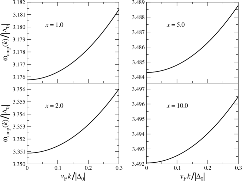
Figure 10: Dispersion relation for the amplitude fluctuation $\omega_{\mathrm{amp}}(k)$ away from the Ginzburg-Landau regime.

Landau damping cut: The imaginary part associated with Landau damping arises for $k\neq 0$ and is nonvanishing only along the Landau damping cut $-v_{\mathrm{F}}k<\omega<v_{\mathrm{F}}k$. Focusing on the long-wavelength, low-frequency limit and in the Ginzburg-Landau regime, we find

$$1+g\widetilde{\Sigma}_{D}(k,s)+g\widetilde{\Sigma}_{O}(k,s) \simeq 2g\left[\Sigma_{O}(0,0)+i\bar{s}x\mathcal{N}(0)I_{c}(\bar{s},x)\right],$$ (131)

where we have used the Ward identity (85) and neglected the contributions from $I_{a,b}$ and $J_{a,b}$, which are subdominant for $v_{\mathrm{F}}k,s\ll|\Delta_{0}|$. We note that in the case of phase fluctuations the terms with $I_{c}$ and $J_{c}$ cancel each other in the difference in the self-energies because $I_{c}=J_{c}$, however, for amplitude fluctuations these terms add up and furnish the dominant contribution.

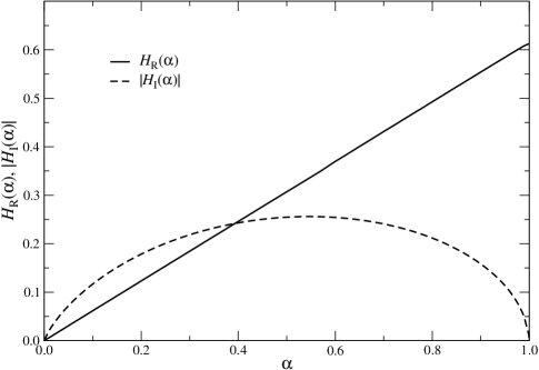
Figure 11: Real and the imaginary parts of $H(\alpha)$.

We now proceed to study the real-time evolution of the amplitude fluctuation by integrating $\widetilde{\delta\rho}_{\mathbf{k}}(s)$ along the Bromwich contour in the complex $s$ plane parallel to the imaginary axis and to the right of all the singularities of the Laplace transform

$$\frac{\widetilde{\delta\rho}_{\mathbf{k}}(s)}{{\delta\rho}_{\mathbf{k}}(0)}=\frac{1}{s}\frac{H(\bar{s},x)}{H(\bar{s},x)+h},$$ (132)

where

$$xh=\Sigma_{O}(0,0)/\mathcal{N}(0),\quad H(\bar{s},x)=i\bar{s}I_{c}(\bar{s},x).$$ (133)

We obtain

$$\delta\rho_{\mathbf{k}}(t)=\int^{\infty}_{-\infty}\frac{d\omega}{\omega}\,\rho_{\mathrm{amp}}(\omega,k)\cos(\omega t)\delta\rho_{\mathbf{k}}(0),$$ (134)

where $\rho_{\mathrm{amp}}(\omega,k)$ is the spectral density for the amplitude fluctuation

$$\rho_{\mathrm{amp}}(\omega,k) = \mathrm{sgn}(\omega)\,Z(k)\,\omega^{2}_{\mathrm{amp}}(k)\,\delta[\omega^{2}-\omega^{2}_{\mathrm{amp}}(k)]+\rho^{\mathrm{cut}}_{\mathrm{amp}}(\alpha),$$

$$\rho^{\mathrm{cut}}_{\mathrm{amp}}(\alpha) = \frac{1}{\pi}\,\mathrm{Im}\left[\frac{h}{h+H(\bar{s},x)}\right]_{\bar{s}=-i\alpha+0^{+}}.$$ (135)

In the above expression the first term arises from quasiparticle pole $\omega_{\mathrm{amp}}(k)$ and the second term arises from the Landau damping cut $-v_{\mathrm{F}}k<\omega<v_{\mathrm{F}}k$.

The quasiparticle pole will contribute an undamped oscillatory component to the time evolution given by

$$\delta\rho^{\mathrm{pole}}_{\mathbf{k}}(t)=Z(k)\cos[\omega_{\mathrm{amp}}(k)t].$$ (136)

The residue of the quasiparticle pole $Z(k)$ is determined by

$$Z(k)=1-\int^{1}_{-1}\frac{d\alpha}{\alpha}\,\rho^{\mathrm{cut}}_{\mathrm{amp}}(\alpha).$$ (137)

Figure 12 shows the temperature dependence of $Z(k)$ in the long-wavelength limit $v_{\mathrm{F}}k\ll|\Delta_{0}|$. It reveals clearly that in the Ginzburg-Landau regime ($x\ll 1$) the spectral density $\rho_{\mathrm{amp}}(k,\omega)$ is dominated by the Landau damping cut.

Whereas the damping rate of the quasiparticle vanishes in the long-wavelength, low-frequency approximation, we expect that higher order contributions, in particular the decay into a pair of Bogoliubov quasiparticles (bogolons) ketterson , will lead to a width of the quasiparticle pole and hence a finite damping rate if the gap the quasiparticle spectrum is greater than $2|\Delta_{0}|$, as seems to be the case from the previous analysis. However, a more comprehensive study of the dispersion relation is needed before reaching a quantitative conclusion. Again this is beyond the regime of validity of the long-wavelength, low-frequency approximation studied here.

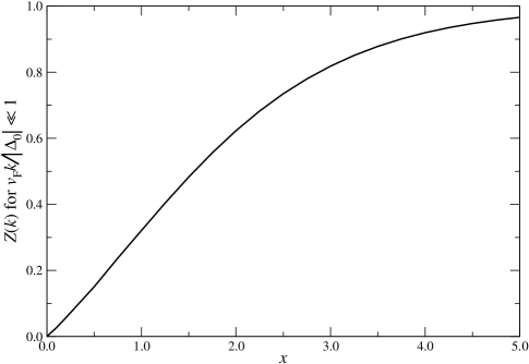
Figure 12: Temperature dependence of the residue for the quasiparticle pole $Z(k)$ in the long-wavelength limit.

In the Ginzburg-Landau regime $x\ll 1$, we find [see (VI)]

$$h=\frac{7\zeta(3)}{8\pi^{2}}x,$$ (138)

and the real and imaginary parts of $H(\bar{s}=-i\alpha+0^{+},0)$ to be given by (here we have set $x=0$)

$$H_{\mathrm{R}}(\alpha) = \frac{\alpha}{8}\int^{\infty}_{0}\frac{dz}{z\epsilon}\ln\left|\frac{\alpha+\frac{z}{\epsilon}}{\alpha-\frac{z}{\epsilon}}\right|,$$

$$\stackrel{{\scriptstyle\alpha\ll 1}}{{\simeq}} \frac{\pi^{2}|\alpha|}{16},$$

$$H_{\mathrm{I}}(\alpha) = -\frac{\pi\alpha}{8}\Theta(1-\alpha^{2})\int_{z_{\mathrm{min}}}^{\infty}\frac{dz}{z\epsilon},$$ (139)

$$\stackrel{{\scriptstyle\alpha\ll 1}}{{\simeq}} -\frac{\pi\alpha}{8}\ln\frac{2}{\alpha},$$

respectively, where $z_{\mathrm{min}}=\sqrt{\alpha^{2}/(1-\alpha^{2})}$. The real and imaginary parts of $H(\alpha)$ are displayed in Fig. 11. The Landau damping contribution to the spectral density in the Ginzburg-Landau regime and the long-wavelength, low-frequency limit is accurately described by

$$\rho^{\mathrm{cut}}_{\mathrm{amp}}(\alpha)=\frac{h\,|H_{\mathrm{I}}(\alpha)|}{\big{[}h+H_{\mathrm{R}}(\alpha)\big{]}^{2}+H^{2}_{\mathrm{I}}(\alpha)}.$$ (140)

which, as displayed in Fig. 13, clearly reveals a sharp peak near $\alpha\approx 0$.

The real-time evolution of the Landau damping contribution to the amplitude fluctuation $\delta\rho^{\mathrm{cut}}_{\mathbf{k}}(t)$ is displayed in Fig. 14. While for $x\lesssim 0.05$ the nonequilibrium relaxation through Landau damping can be approximated by an exponential, clearly such is not the case for $x\gtrsim 0.05$. Nevertheless we still find that the Landau damping relaxation time scale becomes longer as $x\to 0$, revealing that this contribution to the nonequilibrium relaxation seems to be critically slowed down near the critical point.

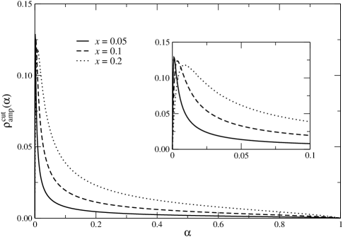
Figure 13: Spectral density $\rho^{\mathrm{cut}}_{\mathrm{amp}}(\alpha)$ vs $\alpha$ in the Ginzburg-Landau regime.

We close this section, by providing the nonlocal Landau damping contribution to the retarded effective action for long-wavelength, low-frequency amplitude fluctuations in the Ginzburg-Landau regime (we have set $J_{\rho}=0$)

$$S^{\mathrm{GL}}_{\mathrm{amp}}[\delta\rho]=2\mathcal{N}(0)\frac{|\Delta_{0}|}{T_{c}}\int d^{3}kd\omega\,\delta\rho_{-\mathbf{k}}(-\omega)\left[\frac{7\zeta(3)|\Delta_{0}|}{8\pi^{2}T}+H(\omega,k)\right]\delta\rho_{\mathbf{k}}(\omega),$$ (141)

up to a additive constant, where $H(\omega,k)=H(\alpha=\omega/v_{\mathrm{F}}k)$ given by (139). Obviously, $S^{\mathrm{GL}}_{\mathrm{amp}}[\delta\rho]$ leads to the retarded equations of motion for the long-wavelength, low-frequency amplitude fluctuations.

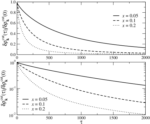
Figure 14: Real-time evolution of the Landau damping contribution to the amplitude fluctuation $\delta\rho^{\mathrm{cut}}_{\mathbf{k}}(t)$ in the Ginzburg-Landau regime is plotted in linear scale (top) and logarithmic scale (bottom).

VII Conclusions

In this article we have focused on the real-time nonequilibrium dynamics of small phase and amplitude fluctuations of the order parameter in neutral BCS superconductors in the Ginzburg-Landau regime near the critical point. We have implemented the Schwinger-Keldysh formulation of nonequilibrium field theory combined with the novel tadpole method to obtain directly in real time the retarded equations of motion for small fluctuations around equilibrium. These equations allow to extract the one-loop effective action for the long-wavelength, low-frequency phase and amplitude fluctuations in the Ginzburg-Landau regime, which is characterized by $|\Delta_{0}(T)|/T\ll 1$ with $\Delta_{0}(T)$ the finite-temperature gap. Furthermore, the retarded equations of motion can be cast as an initial value problem to study the relaxation of nonequilibrium fluctuations directly in real time.

We studied in detail the relaxation of phase fluctuations within and away from the Ginzburg-Landau regime. Despite the fact that the spectral density features a sharp peak with a Goldstone-like dispersion relation in the Ginzburg-Landau regime the relaxation is completely overdamped as a consequence of Landau damping. This is consistent with a purely dissipative time-dependent Ginzburg-Landau equation. However, the effective action is nonlocal because of Landau damping. The relaxation is exponential in time with the damping rate $\gamma_{k}(T)=14\zeta(3)v_{\mathrm{F}}k|\Delta_{0}(T)|/3\pi^{3}T$. The factor $v_{\mathrm{F}}k$ is a consequence of the Goldstone nature of the phase fluctuations. The relaxation of phase fluctuations near the critical point features critical slowing down, i.e., the relaxation time scale diverges at the critical point.

Far away from the Ginzburg-Landau regime at low temperatures, the spectral density features sharp quasiparticle peaks and the nonequilibrium relaxation is underdamped in agreement with the results of Refs. aitchison95, ; aitchison97, . Away from the critical region, the contribution from Landau damping is negligible. The long-wavelength amplitude fluctuations are severely Landau-damped near the critical region and the relaxation time scales also feature critical slowing down.

While we have focused on the nonequilibrium dynamics of neutral BCS superconductors, as a next step we will apply these methods to the case of charged superconductors to study in detail the dynamics of the Carlson-Goldman modes as well as the effective action including gauge fields near the critical temperature. We postpone this study to a forthcoming article.

Appendix A Plane wave solutions and the Bogoliubov transformation

In this Appendix we present an alternative derivation of the correlation functions for the fields $\psi_{\sigma}$, $\psi_{\sigma}^{\dagger}$ directly from the plane wave solutions of the homogeneous equations of motion (i.e., in the absence of source) for the Nambu-Gor’kov field given by (31)

$$\left[i\frac{\partial}{\partial t}+\sigma_{3}\left(\frac{\nabla^{2}}{2m}+\mu\right)+\sigma_{+}\Delta_{0}+\sigma_{-}\Delta_{0}^{\ast}\right]\Psi(\mathbf{x}{},t{})=0.$$ (142)

The plane wave solution can be written in the form

$$\Psi(\mathbf{x}{},t)=\Phi(k)\,e^{-i(\omega t-\mathbf{k}\cdot\mathbf{x}{})},\quad\Phi(k)=\begin{bmatrix}U_{k}\\ V_{k}\end{bmatrix}.$$ (143)

The two-component Nambu-Gor’kov spinor obeys

$$\begin{bmatrix}\xi_{k}&-\Delta_{0}\\ -\Delta_{0}^{\ast}&-\xi_{k}\end{bmatrix}\begin{bmatrix}U_{k}\\ V_{k}\end{bmatrix}=\omega\begin{bmatrix}U_{k}\\ V_{k}\end{bmatrix},$$ (144)

where $\xi_{k}=k^{2}/2m-\mu$. This is an eigenvalue equation with the eigenvalues given by $\omega=\pm E_{k}$, where $E_{k}=\sqrt{\xi^{2}_{k}+|\Delta_{0}|^{2}}$. The normalization of the positive and negative energy spinors is chosen so that $\Phi^{(\alpha)\dagger}(k)\Phi^{(\beta)}(k)=\delta_{\alpha\beta}$, where $\alpha,\beta=1,2$ (not to be confused with the Nambu-Gor’kov indices) correspond to $\omega=\pm E_{k}$, respectively. Introducing the Bogoliubov coefficients $u_{k}$, $v_{k}$ given by

$$u_{k}=\left(\frac{\xi_{k}+E_{k}}{2E_{k}}\right)^{1/2},\quad v_{k}=u_{k}\left(\frac{\Delta_{0}^{\ast}}{\xi_{k}+E_{k}}\right),\quad u_{k}v_{k}=\frac{\Delta_{0}^{\ast}}{2E_{k}},$$ (145)

and satisfying $u_{k}^{2}+|v_{k}|^{2}=1$, we find that the positive and negative energy spinors are given by

$$\Phi^{(1)}(k)=\begin{bmatrix}u_{k}\\ -v_{k}\end{bmatrix},\quad\Phi^{(2)}(k)=\begin{bmatrix}v^{\ast}_{k}\\ u_{k}\end{bmatrix},$$ (146)

respectively. After accounting for the interpretation of negative energy solutions as antiparticles, one can therefore write the general plane wave solution of the homogeneous equation of motion (142) as

$$\Psi(\mathbf{x}{},t)=\frac{1}{\sqrt{V}}\sum_{\mathbf{k}}\left\{b_{\mathbf{k}}\begin{bmatrix}u_{k}\\ -v_{k}\end{bmatrix}e^{-i(E_{k}t-\mathbf{k}\cdot\mathbf{x}{})}+d^{\dagger}_{\mathbf{k}}\begin{bmatrix}v^{\ast}_{k}\\ u_{k}\end{bmatrix}e^{i(E_{k}t-\mathbf{k}\cdot\mathbf{x}{})}\right\},$$ (147)

where $V$ is the quantization volume.

At the level of second quantization, one recognizes that (147) is the Bogoliubov transformation, in which the operator $b^{\dagger}_{\mathbf{k}}$, $d^{\dagger}_{\mathbf{k}}$ create Bogoliubov quasiparticles of momentum $\mathbf{k}$ (energy $E_{k}$) and obey the usual canonical anticommutation relations. The correlation functions of the Nambu-Gor’kov fields in the density matrix that describes free Bogoliubov quasiparticles in thermal equilibrium at inverse temperature $\beta$ are therefore found to be given by (in the continuum limit)

$$\langle\Psi_{a}(\mathbf{x}{},t)\Psi^{\dagger}_{b}(\mathbf{x}{}^{\prime},t^{\prime})\rangle=\int\frac{d^{3}k}{(2\pi)^{3}}\left[[1-n_{\mathrm{F}}(E_{k})]\,\mathcal{S}_{ab}(k)\,e^{-iE_{k}(t-t^{\prime})}+n_{\mathrm{F}}(E_{k})\,\overline{\mathcal{S}}_{ab}(k)\,e^{iE_{k}(t-t^{\prime})}\right]e^{i\mathbf{k}\cdot(\mathbf{x}{}-\mathbf{x}{}^{\prime})},$$

$$\langle\Psi^{\dagger}_{b}(\mathbf{x}{}^{\prime},t^{\prime})\Psi_{a}(\mathbf{x}{},t)\rangle=\int\frac{d^{3}k}{(2\pi)^{3}}\left[n_{\mathrm{F}}(E_{k})\,\mathcal{S}_{ab}(k)\,e^{-iE_{k}(t-t^{\prime})}+[1-n_{\mathrm{F}}(E_{k})]\,\overline{\mathcal{S}}_{ab}(k)\,e^{iE_{k}(t-t^{\prime})}\right]e^{i\mathbf{k}\cdot(\mathbf{x}{}-\mathbf{x}{}^{\prime})},$$

where $n_{\mathrm{F}}(E_{k})$ is the equilibrium distribution for Bogoliubov quasiparticles of momentum $\mathbf{k}$

$$n_{\mathrm{F}}(E_{k})=\langle b^{\dagger}_{\mathbf{k}}b_{\mathbf{k}}\rangle=\langle d^{\dagger}_{\mathbf{k}}d_{\mathbf{k}}\rangle=\frac{1}{e^{\beta E_{k}}+1},$$ (148)

and $\mathcal{S}(k)$, $\overline{\mathcal{S}}(k)$ are given by (45).

References

- (1) E. Abrahams and T. Tsuneto, Phys. Rev. 152, 416 (1966).
- (2) J. Bardeen, L.N. Cooper, and J.R. Schrieffer, Phys. Rev. 108, 1175 (1957).
- (3) P.G. de Gennes, Superconductivity of metals and alloys (Addison-Wesley, Redwood City, C.A., 1989).
- (4) V.I. Ginzburg and L.D. Landau, Zh. Eksp. Teor. Fiz. 20, 1064 (1950).
- (5) L.P. Gor’kov, Sov. Phys. JETP 9, 1364 (1959).
- (6) A. Fetter and J. Walecka, Quantum Theory of Many-Particle Systems (McGraw-Hill, New York, 1971).
- (7) C.M. Fraser, Z. Phys. C 28, 101 (1985).
- (8) M. Greiter, F. Wilczek and E. Witten, Mod. Phys. Lett. B 3, 903 (1989).
- (9) A.M.J. Schakel, Mod. Phys. Lett. B 4, 927 (1990).
- (10) I.J.R. Aitchison, P. Ao, D.J. Thouless, and X.M. Zhu, Phys. Rev. B 51, 6531 (1995).
- (11) M. Stone, Int. J. Mod. Phys. B 9, 1359 (1995).
- (12) S.D. Palo, C. Castellani, C.D. Castro and B.K. Chakraverty, Phys. Rev. B 60, 564 (1999).
- (13) H.T.C. Stoof, Phys. Rev. B 47, 7979 (1992).
- (14) I.J.R. Aitchison and D.J. Lee, Phys. Rev. B 56, 8303 (1997); I.J.R. Aitchison, G. Metikas, and D.J. Lee, Phys. Rev. B 62, 6638 (2000).
- (15) N.P. Kopnin, J. Low Temp. Phys. 97, 157 (1994).
- (16) R.J. Watts-Tobin, Y. Krahenbuhl and L. Kramer, J. Low Temp. Phys. 42, 459 (1981).
- (17) S.G. Sharapov, H. Beck, and V.M. Loktev, Phys. Rev. B 64, 134519 (2001); S.G. Sharapov and H. Beck, Phys. Rev. B 65 134516 (2002).
- (18) Y. Ohashi and S. Takada, Phys. Rev. B 62, 5971 (2000); K.Y.M. Wong and S. Takada, Phys. Rev. B 37, 5644 (1988).
- (19) A. Paramekanti, M. Randeria, T.V. Rmakrishnan, and S.S. Mandal, Phys. Rev. B 62, 6786 (2000).
- (20) L. Benfatto, A.Toschi, S. Caprara, and C. Castellani, Phys. Rev. B 64, 140506 (2001).
- (21) R.V. Carlson and A.M. Goldman, Phys. Rev. Lett. 31, 880 (1973); J. Low Temp. Phys. 25, 67 (1976); F.E. Aspen and A.M. Goldman, J. Low Temp. Phys. 43, 559 (1981).
- (22) V.M. Loktev, R.M. Quick, and S.G. Sharapov, Phys. Rep. 349, 1 (2001).
- (23) F. Schreck, L. Khaykovich, K.L. Corwin, G. Ferrari, T. Bourdel, J. Cubizolles, and C. Salomon, A quasi-pure Bose Einstein condensate immersed in a Fermi sea, cond-mat/0107442 (2001); F. Schreck, G. Ferrari, K.L. Corwin, J. Cubizolles, L. Khaykovich, M.-O. Mewes, and C. Salomon, Sympathetic cooling of bosonic and fermionic Lithium gases towards quantum degeneracy, cond-mat/0011291 (2000).
- (24) H.T.C. Stoof, M. Houbiers, C. A. Sackett, and R.G. Hulet, Phys. Rev. Lett. 76, 10 (1996).
- (25) G. M. Bruun and B. R. Mottelson, Phys. Rev. Lett. 87, 270403 (2001).
- (26) F. Zambelli and S. Stringari, cond-matt/0004325 (2000), A. Minguzzi and M.P. Tosi, Phys. Rev. A 63, 023609 (2001); G.M. Bruun and C.W. Clark, J. Phys. B 33, 3953 (2000). G. Bruun, Y. Castin, R. Dum, K. Burnett, Euro. Phys. J. D 7, 433 (1999); G.M. Bruun and H. Heiselberg Phys. Rev. A 65, 053407 (2002).
- (27) C.J. Pethick and H. Smith, Bose-Einstein Condensation in Dilute Gases (Cambridge University Press, Cambridge, 2002), see section 14.
- (28) J. Schwinger, J. Math. Phys. 2, 407 (1961); L.V. Keldysh, Sov. Phys. JETP 20, 1018 (1965); K.-C. Chou, Z.-B. Su, B.-L. Hao, and L. Yu, Phys. Rep. 118, 1 (1985); J. Rammer and H. Smith, Rev. Mod. Phys. 58, 323 (1986); E. Lifschitz and L. Pitaevskii, Physical Kinetics (Pergamon Press, Oxford, 1981).
- (29) For simplicity of presentation, we consider here only the generating functional for the Nambu-Gor’kov fields and , whose Green’s functions will enter explicitly in the equations of motion for the condenstate perturbation. The inclusion of the (bosonic) pair fields and in the generating functional is straightforward.
- (30) L.P. Kadanoff and G. Baym, Quantum Statistical Mechanics (W.A. Benjamin, New York, 1962).
- (31) See, for example, D. Boyanovsky, H.J. de Vega, R. Holman, and D.-S. Lee, Phys. Rev. D 52, 6805 (1995); D. Boyanovsky, M. D’Attanasio, H.J. de Vega, and R. Holman, 54, 1748 (1996); and references therein.
- (32) J.W. Negele and H. Orland, Quantum Many-Particle Systems (Perseus Books, Reading, M.A., 1998).
- (33) D. Boyanovsky, H.J. de Vega, D.-S. Lee, Y.J. Ng, and S.-Y. Wang, Phys. Rev. D 59, 105001 (1999); S.-Y. Wang, D. Boyanovsky, H.J. de Vega, D.-S. Lee, and Y.J. Ng, 61, 065004 (2000); S.-Y. Wang, D. Boyanovsky, H.J. de Vega, and D.-S. Lee, 62, 105026 (2000). For the description of nonequilibrium methods in quantum field theory see, for example, D. Boyanovsky, H.J. de Vega, and R. Holman, in Proceedings of the Second Paris Cosmology Colloquium, edited by H.J. de Vega and N. Sanchez, (World Scientific, Singapore, 1995), hep-th/9412052; and references therein.
- (34) N.V. Mikheev and N.V. Chistyakov, JETP Lett. 73, 642 (2001).
- (35) D. Boyanovsky, S.-Y. Wang, D.-S. Lee, H.-L. Yu, and S.M. Alamoudi, cond-mat/0111375 (Ann. Phys. in press).
- (36) Y. Nambu, Phys. Rev. 117, 648 (1960); L.P. Gor’kov, Sov. Phys. JETP 7, 505 (1958).
- (37) See, J.B. Ketterson and S.N. Song, Superconductivity (Cambridge University Press, 1999), Sec. 45.
- (38) Up to an overall factor, the expression for coincides with the limit of Eq. (39) in the second reference in Ref. aitchison97, for .
- (39) In the first reference in Ref. aitchison97, , it is found that the value of the gap is [see Eq. (31) in that reference].