Universal properties of cuprate superconductors: Evidence and implications

Abstract

To be published in:

The Physics of Conventional and Unconventional Superconductors

Springer-Verlag, Berlin, ed. K.H. Bennemann and J.B. Ketterson

I Introduction

Establishing and understanding the phase diagram of cuprate superconductors in the temperature - dopant concentration plane is one of the major challenges in condensed matter physics. Superconductivity is derived from the insulating and antiferromagnetic parent compounds by partial substitution of ions or by adding or removing oxygen. For instance La₂CuO₄ can be doped either by alkaline earth ions or oxygen to exhibit superconductivity. The empirical phase diagram of La_2-xSr_xCuO₄ [2, 3, 4, 5, 6, 7, 8, 9, 10] depicted in Fig.1 shows that after passing the so called underdoped limit $\left(x_{u}\approx 0.047\right)$, $T_{c}$ reaches its maximum value $T_{c}^{m}$ at $x_{m}\approx 0.16$. With further increase of $x$, $T_{c}$ decreases and finally vanishes in the overdoped limit $x_{o}\approx 0.273$. This phase transition line is thought to be a generic property of cuprate superconductors [11]  and is well described by the empirical relation

$$T_{c}\left(x\right)=T_{c}\left(x_{m}\right)\left(1-2\left(\frac{x}{x_{m}}-1\right)^{2}\right)=\frac{2T_{c}\left(x_{m}\right)}{x_{m}^{2}}\left(x-x_{u}\right)\left(x_{o}-x\right),\ \ x_{m}=0.16,$$ (1)

proposed by Presland et al.[12]. Approaching the endpoints along the axis $x$, La_2-xSr_xCuO₄ undergoes at zero temperature doping tuned quantum phase transitions. As their nature is concerned, resistivity measurements reveal a quantum superconductor to insulator (QSI) transition in the underdoped limit[4, 13, 14, 15, 16] and in the overdoped limit a quantum superconductor to normal state (QSN) transition[16].

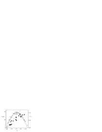
FIG. 1.: Variation of $T_{c}$ (open circles) [2, 3, 4, 5, 6, 7, 8, 9, 10] and $\gamma_{T}$ with $x$ for La_2-xSr_xCuO₄. Filled circles correspond to $1/\gamma_{T_{c}}$ [2, 3, 5, 7, 8] and filled triangles to $1/\gamma_{T=0}$ [9, 10]. The solid curve is Eq.(1) with $T_{c}^{m}=39K$. The dashed and dotted lines follow from Eq.(2) with $\gamma_{0,T_{c}}=2$ and $\gamma_{T_{c}}=1.63$.

Another essential experimental fact is the doping dependence of the anisotropy. In tetragonal cuprates it is defined as the ratio $\gamma=\xi_{ab}/\xi_{c}$ of the correlation lengths parallel $\left(\xi_{ab}\right)$ and perpendicular $\left(\xi_{c}\right)$ to CuO₂ layers (ab-planes). In the superconducting state it can also be expressed as the ratio $\gamma=\lambda_{c}/\lambda_{ab}$ of the London penetration depths due to supercurrents flowing perpendicular ($\lambda_{c}$ ) and parallel ($\lambda_{ab}$ ) to the ab-planes. Approaching a nonsuperconductor to superconductor transition $\xi$ diverges, while in a superconductor to nonsuperconductor transition $\lambda$ tends to infinity. In both cases, however, $\gamma$ remains finite as long as the system exhibits anisotropic but genuine 3D behavior. There are two limiting cases: $\gamma=1$ characterizes isotropic 3D- and $\gamma=\infty$ 2D-critical behavior. An instructive model where $\gamma$ can be varied continuously is the anisotropic 2D Ising model[17]. When the coupling in the y direction goes to zero, $\gamma=\xi_{x}/\xi_{y}$ becomes infinite, the model reduces to the 1D case and $T_{c}$ vanishes. In the Ginzburg-Landau description of layered superconductors the anisotropy is related to the interlayer coupling. The weaker this coupling is, the larger $\gamma$ is. The limit $\gamma=\infty$ is attained when the bulk superconductor corresponds to a stack of independent slabs of thickness $d_{s}$. With respect to experimental work, a considerable amount of data is available on the chemical composition dependence of $\gamma$ . At $T_{c}$ it can be inferred from resistivity ($\gamma=\xi_{ab}/\xi_{c}=\sqrt{\rho_{ab}/\rho_{c}}$) and magnetic torque measurements, while in the superconducting state it follows from magnetic torque and penetration depth ($\gamma=\lambda_{c}/\lambda_{ab}$) data. In Fig.1 we included the doping dependence of $1/\gamma_{T}$ evaluated at $T_{c}$ ($\gamma_{T_{c}}$) and $T=0$ ($\gamma_{T=0}$). As the dopant concentration is reduced, $\gamma_{T_{c}}$ and $\gamma_{T=0}$ increase systematically, and tend to diverge in the underdoped limit. Thus the temperature range where superconductivity occurs shrinks in the underdoped regime with increasing anisotropy. This competition between anisotropy and superconductivity raises serious doubts whether 2D mechanisms and models, corresponding to the limit $\gamma_{T}=\infty$, can explain the essential observations of superconductivity in the cuprates. From Fig.1 it is also seen that $\gamma_{T}\left(x\right)$ is well described by

$$\gamma_{T}\left(x\right)=\frac{\gamma_{T,0}}{x-x_{u}}.$$ (2)

Having also other cuprate families in mind, it is convenient to express the dopant concentration in terms of $T_{c}$. From Eqs.(1) and(2) we obtain the correlation between $T_{c}$ and $\gamma_{T}$:

$$\frac{T_{c}}{T_{c}\left(x_{m}\right)}=1-\left(\frac{\gamma_{T}\left(x_{m}\right)}{\gamma_{T}}-1\right)^{2},\ \ \gamma_{T}\left(x_{m}\right)=\frac{\gamma_{T,0}}{x_{m}-x_{u}}$$ (3)

Provided that this empirical correlation is not merely an artefact of La_2-xSr_xCuO₄, it gives a universal perspective on the interplay of anisotropy and superconductivity, among the families of cuprates, characterized by $T_{c}\left(x_{m}\right)$ and $\gamma_{T}\left(x_{m}\right)$. For this reason it is essential to explore its generic validity. In practice, however, there are only a few additional compounds, including HgBa₂CuO_4+δ[18] and Bi₂Sr₂CuO_6+δ, for which the dopant concentration can be varied continuously throughout the entire doping range. It is well established, however, that the substitution of magnetic and nonmagnetic impurities, depress $T_{c}$ of cuprate superconductors very effectively[19, 20]. To compare the doping and substitution driven variations of the anisotropy, we depicted in Fig.2 the plot $T_{c}/T_{c}\left(x_{m}\right)$ versus $\gamma_{T}\left(x_{m}\right)/$ $\gamma_{T}$ for a variety of cuprate families. The collapse of the data on the parabola, which is the empirical relation (3), reveals that this scaling form appears to be universal. Thus, given a family of cuprate superconductors, characterized by $T_{c}\left(x_{m}\right)$ and $\gamma_{T}\left(x_{m}\right)$, it gives a universal perspective on the interplay between anisotropy and superconductivity.

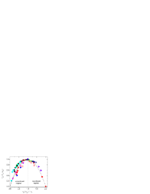
FIG. 2.: $T_{c}/T_{c}\left(x_{m}\right)$ versus $\gamma_{T}\left(x_{m}\right)/$ $\gamma_{T}$ for La_2-xSr_xCuO₄ ($\bullet$, $T_{c}\left(x_{m}\right)=37K$, $\gamma_{T_{c}}\left(x_{m}\right)=20$) [2, 3, 5, 7, 8] , ($\bigcirc$, $T_{c}\left(x_{m}\right)=37K$, $\gamma_{T=0}\left(x_{m}\right)=14.9$) [9, 10], HgBa₂CuO_4+δ ($\blacktriangle$, $T_{c}\left(x_{m}\right)=95.6K$, $\gamma_{T_{c}}\left(x_{m}\right)=27$) [18], Bi₂Sr₂CaCu₂O_8+δ ($\bigstar$, $T_{c}\left(x_{m}\right)=84.2K$, $\gamma_{T_{c}}\left(x_{m}\right)=133$)[21], YBa₂Cu₃O_7-δ ($\blacklozenge$, $T_{c}\left(x_{m}\right)=92.9K$, $\gamma_{T_{c}}\left(x_{m}\right)=8$) [22], YBa₂(Cu_1-yFe_y)₃O_7-δ ($\blacksquare$, $T_{c}\left(x_{m}\right)=92.5K$, $\gamma_{T_{c}}\left(x_{m}\right)=9$)[23], Y_1-yPr_yBa₂Cu₃O_7-δ ($\blacktriangledown$, $T_{c}\left(x_{m}\right)=91K$, $\gamma_{T_{c}}\left(x_{m}\right)=9.3$)[24], BiSr₂Ca_1-yPr_yCu₂O₈ ($\blacktriangleleft$, $T_{c}\left(x_{m}\right)=85.4K$, $\gamma_{T=0}\left(x_{m}\right)=94.3$) [25] and YBa₂(Cu_1-y Zn_y)₃O_7-δ ($\blacktriangleright$, $T_{c}\left(x_{m}\right)=92.5K$, $\gamma_{T=0}\left(x_{m}\right)=9$) [26]. The solid and dashed curves are Eq.(18), marking the flow from the maximum $T_{c}$ to QSI and QSN criticality, respectively.

The effect of a substitution for Cu by other magnetic or nonmagnetic metals was also investigated extensively [16, 19, 20]. A result common to all of these studies is that $T_{c}$ is suppressed in the same manner, independent of wether the substituent is magnetic or nonmagnetic. For this reason, the phase diagram of  La_2-xSr_xCu_1-yZn_yO₄, depicted in Fig.3, applies quite generally. Apparently, the substituent axis (y) extends the complexity and richness of the phase diagram considerably. The blue curve corresponds to a line of quantum phase transitions, given by $y_{c}\left(x\right)$. The pink arrow marks the doping tuned insulator to metal crossover and the green arrow corresponds to a path along which a QSI and QSN transition occurs. From Fig. 4 it can be inferred that isotope substitution, though much less effective, has essentially the same effect. $T_{c}$ is lowered and the underdoped limit $x_{u}$ shifts to some $y_{c}\left(x\right)$. This suggests that substitution induced local distortions, rather than magnetism, is the important factor. For $y>y_{c}\left(x\right)$ superconductivity is suppressed due to the destruction of phase coherence.

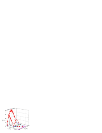
FIG. 3.: Phase diagram of  La_2-xSr_xCu_1-yZn_yO₄ . The blue solid curve corresponds to $y_{c}\left(x\right)$, a line of quantum phase transitions. The pink arrow marks the doping tuned insulator to metal crossover and the green arrow marks a path where a QSI and QSN transition occurs. Experimental data taken from Momono et al. [16].

FIG. 4.: $T_{c}$ (¹⁶O ) and $T_{c}$ (¹⁸O ) versus $x$ for La_2-xSr_xCuO₄ . From Guo-Meng Zhao et al.[27].

The point of reference for magnetic field tuned transitions is embodied in the schematic phase diagram  shown in Fig.5. It is strongly affected by the combined effect of pinning, thermal and quantum fluctuations, anisotropy and dimensionality [28]. In clean cuprates and close to $T_{c}\left(x,H=0\right)$ thermal fluctuations are thought to be responsible for the existence of a first-order vortex melting transition. In the presence of disorder, however, the long-range order of the vortex lattice is destroyed and the vortex solid becomes a glass [29]. Since a sufficiently large magnetic field suppresses superconductivity, due to the destruction of phase coherence, there is a line $H_{m}\left(x\right)$ of quantum phase transitions, connecting the zero field QSI and QSN transitions. Indeed, recent experiments revealed that sufficiently-intense magnetic fields suppress superconductivity and mediate a metal to insulator (MI) crossover [30, 31, 32, 33].

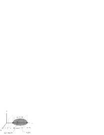
FIG. 5.: Schematic ($x,H,T$)-phase diagram. There is the superconducting phase (S), bounded by the zero-field transition line, $T_{c}\left(x,H=0\right)$, the critical lines of  the vortex melting or vortex glass to vortex fluid transitions,  $T_{m}\left(x=\text{fixed},H\right)$ and the line of quantum critical points, $H_{m}\left(x,T=0\right)$. Along this line superconductivity is suppressed and the critical endpoints coincide with the 2D-QSI- and 3D-QSN- critical points at $x_{u}$ and $x_{o}$, respectively.

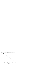
FIG. 6.: Zero resistance $T_{c}$ versus $1/d$  of YBa₂Cu₃O${}_{7-\delta\text{ }}$ layers of thickness $d$ separated by 16 PrBa₂Cu₃O${}_{7\text{ }}$unit cells. Taken from Goodrich et al. [34]. The straight line is a linear fit to Eq.(4).

The QSI transition can also be traversed in films by changing their thickness[14]. An instructive example are the measurements on YBa₂Cu₃O_7-δ slabs of thickness $d$ separated by 16 unit cells ($\approx 187\ A$) of PrBa₂Cu₃O₇. Due to their large separation the YBa₂Cu₃O_7-δ slabs are essentially uncoupled. As shown in Fig.6, $T_{c}$ was found to vary with the thickness $d$ of the YBa₂Cu₃O_7-δ slabs as

$$\frac{T_{c}\left(d\right)}{T_{c}^{bulk}}=\frac{d_{s}}{d}\left(\frac{d}{d_{s}}-1\right),$$ (4)

with $T_{c}^{bulk}=91\ K$ and $d_{s}=10.1\ A$[34]. $d_{s}$ is the critical film thickness below which superconductivity is lost. Although the decrease of $T_{c}$ is partially due to the 3D-2D crossover, the occurrence of the QSI transition points to the dominant role of disorder and quantum fluctuations. For this reason it is conceivable that in sufficiently clean films superconductivity may also occur at and slightly below $d_{s}$. Recently this has been achieved by inducing charges by the field-effect technique, whereby the mobile carrier density can be varied continuously and reversibly, without introducing additional sources of disorder[35, 36, 37]. By establishing a voltage difference between a metallic electrode and the crystal, charge can be added or removed from the CuO₂ layers: positive voltage injects electrons, and a negative voltage injects holes. This allows to vary both electron and hole charge densities over a considerable range of interest. Using this technique Schön et al.[37] converted an insulating thin slab of  CaCuO₂ into a superconductor. The success of this technique relies on the high quality films and on the quality of the interfaces between the film material and the metallic electrode. The ($T_{c}$, $x$) phase diagram for CaCuO₂ is shown Fig.7. The doping level was calculated from the independently measured capacitance of the gate dielectric, assuming that all the charge is located in a single CuO₂ layer. The diagram exhibits apparent electron and hole superconductivity, and bears a strong resemblance to results observed in other cuprates, in qualitative agreement with the empirical correlation (3) for bulk systems. Note that the finite temperature superconductor to normal state transition falls into the 2D-XY universality class. Thus $T_{c}$ is the Kosterlitz-Thouless transition temperature. At low doping levels ($x<0.1$) a logarithmic divergence of the resistivity was found. This observation for n- as well as p-type doping of CaCuO₂ are in accordance with a 2D-QSI transition in the underdoped limit. Although superconductivity has been observed previously in SrCuO₂/BaCuO₂[38] and in BaCuO₂/CaCuO₂[39] superlattices with a maximum $T_{c}$ value of about 80 K, the field effect doping is not limited by dopant solubility and compositional stability. This technique allows to study the properties of a given material as a function of the dopant concentration without introducing additional disorder and additional defects. Because the charge carriers appear to be confined in a very thin layer, what’s seen is superconductivity in 2D. Thus, due to the reduced dimensionality fluctuations will be enhanced over the full range of dopant concentrations. The phase diagram displayed in Fig.7 also points to a 2D-QSN transition in the overdoped limit. In any case, this phase diagram clearly reveals the survival of superconductivity in field effect doped CaCuO₂ in the 2D-limit, while it disappears in the bulk (see e.g. Fig.2) with increasing anisotropy and in chemically doped films at a critical thickness $d_{s}$, presumably controlled by disorder.

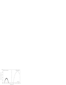
FIG. 7.: ($T_{c}$, $x$) phase diagram of CaCuO₂. A maximum $T_{c}$ of $89$ and $34$ K is obtained at optimal hole and electron doping, respectively. Doping level x is defined as number of charge carriers per CuO₂ unit. Taken from Schön et al.[37].

This review aims to analyze the empirical correlations and phase diagrams from the point of view of thermal and quantum critical phenomena, to identify the universal properties, the effective dimensionality and the associated crossover phenomena. In view of the mounting evidence for 3D-XY-universality close to optimum doping [8, 14, 40, 41, 42, 43, 44, 45, 46], we concentrate here on the thermodynamic and ground state properties emerging from the QSI- and QSN- transitions, including the associated crossover phenomena. For this purpose we invoke the scaling theory of quantum critical phenomena[14, 47].

Zero temperature phase transitions in quantum systems differ fundamentally from their finite temperature counterparts in that their thermodynamics and dynamics are inextricably mixed. Nevertheless, by means of the path integral formulation of quantum mechanics, one can view the statistical mechanics of D-dimensional $T=0$ quantum system as the statistical mechanics of a $D+z$ dimensional classical system with a fake temperature which is some measure of the dynamics, characterized by the dynamic critical exponent $z$. This allows one to apply the scaling theory developed for classical critical phenomena to quantum criticality. In particular this leads to an understanding of the low $T$ and crossover behavior close to quantum phase transitions and to universal relations between various properties. Evidence for power law behavior should properly consist of data that cover several decades in the parameters to provide reliable estimates for the critical exponents. In cuprate superconductors, the various power laws span at best one decade. Accordingly, more extended experimental data are needed to determine the critical exponents of the quantum phase transitions. Nevertheless, irrespective of their precise value, the evidence for scaling and with that for data collapse exists. It uncovers the relationship between various properties and the significance of the empirical correlations and offers an understanding of the doping, substitution and magnetic field tuned quantum phase transition points and lines (see Figs.1, 3 and 5). Evidently, the anisotropy, the associated dimensional crossover and the scaling relations between various properties close to the OSI and QSN criticality provide essential constraints for the understanding of the phase diagrams and the microscopic theory of superconductivity in these materials.

Note that this scenario is not incompatible with the zoo of microscopic models, relying on competing order parameters [48, 49, 50, 51, 52, 53, 54, 55, 56, 57, 58]. Here it is assumed that in the doping regime where superconductivity occurs, competing fluctuations, including antiferromagnetic and charge fluctuations, can be integrated out. The free-energy density is then a functional of a complex scalar, the order parameter of the superconducting phase, only. Given the generic phase diagrams (Figs.1, 3 and 5) the scaling theory of finite temperature and quantum critical phenomena leads to predictions, including the universal properties, which can be confronted with experiment. As it stands, the available experimental data appears to be fully consistent with a single complex scalar order parameter, a doping tuned dimensional crossover and a doping, substitution or magnetic field driven suppression of superconductivity, due to the loss of phase coherence. When the evidence for this scenario persists, antiferromagnetic and charge fluctuations turn out to be irrelevant close to criticality. Moreover, it implies that a finite transition temperature and superfluid aerial superfluid density in the ground state, require in chemically doped systems a finite anisotropy. The important conclusion there is that a finite superfluid density in the ground state of bulk cuprates oxides is unalterably linked to an anisotropic but 3D condensation mechanism. Thus despite the strongly two-dimensional layered structure of cuprate superconductors, a finite anisotropy associated with the third dimension, perpendicular to the CuO₂ planes, is an essential factor in mediating superfluidity.

The paper is organized as follows. Sec.II is devoted to the finite temperature critical behavior. Since a substantial review on this topic is available[14], we concentrate on the specific heat. In Sec.II.A we sketch the scaling theory of finite temperature critical phenomena in anisotropic superconductors falling into the 3D-XY universality class. This leads naturally to universal critical amplitude combinations, involving the transition temperature and the critical amplitudes of specific heat, correlation lengths and penetration depths. The universality class to which the cuprates belong is thus not only characterized by its critical exponents but also by various critical-point amplitude combinations which are equally important. Indeed, though these amplitudes depend on the dopant concentration, substitution etc., their universal combinations do not. Evidence for 3D-XY universality and their implication for the vortex melting transition is presented in Sec.II.B. Here we also discuss the limitations arising from the inhomogeneities and the anisotropy, which render it difficult to observe 3D-XY critical behavior along the entire phase transition line $T_{c}\left(x\right)$ (Fig.1) or on the entire surface $T_{c}\left(x,y\right)$ (Fig.3).

In Sec.III we examine the quantum phase transitions and the associated crossover phenomena. The scaling theory of quantum phase transitions[47], extended to anisotropic superconductors[14], is reviewed in Sec.III.A. Essential predictions include a universal amplitude relation in D=2 involving the transition temperature and the zero temperature in-plane penetration depth, as well as a fixed value of the in-plane sheet conductivity. Moreover we explore the scaling properties of transition temperature, penetration depths, correlation lengths, anisotropy and specific heat coefficient at 2D-QSI and 3D-QSN criticality. In Sec.III.B we confront these predictions with the empirical correlations (1), (2) and (3) and pertinent experiments. Although the experimental data are rather sparse, in particular close to the 3D-QSN transition, we observe a flow pattern pointing consistently to a 2D-QSI transition with $z=1$ and $\overline{\nu}\approx 1$, and 3D-QSN criticality with $z=2$ and $\overline{\nu}\approx 1/2$. $z$ is the dynamic critical exponent and $\overline{\nu}$ the correlation length exponent. The estimates for the 2D-QSI transition coincide with the theoretical prediction for a 2D disordered bosonic system with long-range Coulomb interactions[59, 60]. This reveals that in cuprate superconductors the loss of phase coherence, due to the localization of Cooper pairs, is responsible for the 2D-QSI transition. On the other hand, $z=2$ and $\overline{\nu}\approx 1/2$ point to a 3D-QSN critical point, compatible with a disordered metal to d-wave superconductor transition at weak coupling[61]. Here the disorder destroys superconductivity, while at the 2D-QSI transition it destroys superfluidity. A characteristic feature of the 2D-QSI transition is its rather wide and experimentally accessible critical region. For this reason we observe consistent evidence that it falls into the same universality class as the onset of superfluidity in ⁴He films in disordered media, corrected for the long-rangeness of the Coulomb interaction. As also discussed in this section, the existence of 2D-QSI and 3D-QSN critical points implies a doping and substitution tuned dimensional crossover. A glance to Fig.2 shows that it is due to the dependence of the anisotropy on doping and substitution. An important implication is, that despite the small fraction, which the third dimension contributes to the superfluid energy density in the ground state, a finite transition temperature and superfluid density in bulk cuprates is unalterably linked to a finite anisotropy. Thus, despite their strongly two-dimensional layered structure, a finite anisotropy associated with the third dimension, perpendicular to the CuO₂ planes, is an essential factor in mediating pair condensation. This points unambiguously to the conclusion that theories formulated for a single CuO₂ plane cannot be the whole story. Moreover, the evidence for the flow to 2D-QSI criticality also implies that the standard Hamiltonian for layered superconductors[62] is incomplete. Although its critical properties fall into the 3D-XY universality class, disorder and quantum fluctuations must be included to account for the flow to 2D-QSI and 3D-QSN criticality.

Sec.IV is devoted to the magnetic field tuned quantum phase transitions. Contrary to finite temperature, disorder is an essential ingredient at $T=0$. It destroys superconductivity at 3D-QSN criticality and superfluidity at 2D-QSI critical points. On the other hand, superconductivity is also destroyed by a sufficiently large magnetic field. Accordingly, one expects a line $H_{m}\left(x\right)$ of quantum phase transitions, connecting the zero field 2D-QSI and 3D-QSN transitions (see Fig.5). The relevance of disorder at this critical endpoints suggests a line of quantum vortex glass to vortex fluid transitions. Although the available experimental data is rather sparse, it points to the existence of a quantum critical line $H_{m}\left(x\right)$ and 2D localization, consistent with 2D-QSI criticality.

In Sec.V we treat cuprates with reduced dimensionality. Empirically it is well established that a quantum superconductor to insulator transition in thin films can also be traversed by reducing the film thickness. There is a critical film thickness ($d_{s}$) where $T_{c}$ vanishes and below which disorder destroys superconductivity[14]. In chemically doped cuprates the critical thickness is comparable to the c-axis lattice constant. Moreover, the empirical correlation (3), displayed in Fig.2, implies that in the bulk superconductivity disappears in the 2D limit. Thus, the combined effect of disorder and quantum fluctuations appears to prevent the occurrence of strictly 2D superconductivity. For this reason it is conceivable that in sufficiently clean films superconductivity may also occur at and below this value of $d_{s}$. As aforementioned, this has been achieved by field effect doped CaCuO₂[37]. Although more detailed studies are needed to uncover the characteristic 2D critical properties in field effect doped cuprates, the phase diagram of CaCuO₂ clearly points to a 2D-QSI transition in the underdoped and a 2D-QSN transition in the overdoped limit. It also implies that in field effect doped cuprates superconductivity survives in the 2D limit, while in the bulk and chemically doped films it disappears. Since chemically doped materials with different carrier densities also have varying amounts of disorder, the third dimension appears to be needed to delocalize the carriers and to mediate superfluidity. The comparison with other layered superconductors, including organics and dichalcogenides is made in Sec.VI.

II Finite temperature critical behavior

A Sketch of the scaling predictions

In superconductors the order parameter is a complex scaler, but it can also be viewed as a two component vector (XY). Supposing that sufficiently close to the phase transition line, separating the superconducting and non superconducting phase, 3D-XY-fluctuations dominate, the scaling form of the singular part of the bulk free energy density adopts then the form [14, 63]

$$f_{s}=-k_{B}TQ_{3}^{\pm}\left(\xi_{x}^{\pm}\xi_{y}^{\pm}\xi_{z}^{\pm}\right)^{-1}$$ (5)

where $\xi_{i}^{\pm}$ is the correlation length diverging as

$$\xi_{i}^{\pm}=\xi_{i,0}^{\pm}\left|t\right|^{-\nu},\ i=x,y,z,\ \pm\ =sign\left(t\right),\ \ t=\frac{T-T_{c}}{T_{c}}$$ (6)

and $Q_{3}^{\pm}$ are universal constants. In this context it should be kept in mind, that in superconductors the pairs carry a non zero charge in addition to their mass and the charge $\left(\Phi_{0}=hc/2e\right)$ couples the order parameter to the electromagnetic field via the gradient term in the Ginzburg-Landau Hamiltonian. In extreme type II superconductors, however, the coupling to vector potential fluctuations appears to be weak[64], but nonetheless, in principle, these fluctuations drive the system very close to criticality, to a charged critical point[66]. In any case, inhomogeneities in cuprate superconductors appear to prevent from entering this regime, due to the associated finite size effect[14]. For these reasons, the neglect of vector potential fluctuations appears to be justified and the critical properties at finite temperature are then those of the 3D-XY - model, reminiscent to the lamda transition in superfluid helium, extended to take the anisotropy into account[14, 40].

In the superconducting phase the order parameter $\Psi$ can be decomposed into a longitudinal ($\Psi_{0}+\Psi_{lo}$) and transverse ($\Psi_{tr}$) part:

$$\Psi=\Psi_{0}+\Psi_{lo}+i\Psi_{tr},$$ (7)

where $\Psi_{0}=\left\langle\Psi\right\rangle$ is chosen to be real. At long wavelength and in the superconducting phase the transverse fluctuations dominate and the correlations do not decay exponentially, but according to a power law[14, 63]. This results in an inapplicability of the usual definitions of a correlation length below $T_{c}$. However, in terms of the helicity modulus, which is a measure of the response of the system to a phase-twisting field, a phase coherence length can be defined[65]. This length diverges at critical points and plays the role of the standard correlation length below $T_{c}$. In the presence of a phase twist of wavenumber $k_{i}$, the singular part of the free energy density adopts the scaling form

$$f_{s}=-\frac{k_{B}TQ_{3}^{-}}{\xi_{x}^{tr}\xi_{y}^{tr}\xi_{z}^{tr}}\Phi\left(k_{x}\sqrt{\xi_{y}^{tr}\xi_{z}^{tr}},k_{y}\sqrt{\xi_{x}^{tr}\xi_{z}^{tr}},k_{z}\sqrt{\xi_{x}^{tr}\xi_{y}^{tr}}\right),$$ (8)

yielding for the helicity modulus the expression

$$\Upsilon_{i}=-=\left.\frac{\partial^{2}f_{s}}{\partial k_{i}^{2}}\right|_{{\bf k}={\bf 0}}=\frac{k_{B}TQ_{3}^{-}}{\xi_{i}^{tr}}\left.\frac{\partial^{2}\Phi}{\partial k_{i}^{2}}\right|_{{\bf k}={\bf 0}}$$ (9)

where the normalization, $Q_{3}^{-}\left(\partial^{2}\Phi/\partial k_{i}^{2}\right)_{{\bf k}={\bf 0}}$ $=1$, has been chosen. At $T_{c}$ this leads to the universal relation

$$\left(k_{B}T_{c}\right)^{3}=\xi_{x0}^{tr}\xi_{y0}^{tr}\xi_{z0}^{tr}\Upsilon_{x0}\Upsilon_{y0}\Upsilon_{z0}=\left(\frac{\Phi_{0}^{2}}{16\pi^{3}}\right)^{3}\frac{\xi_{x0}^{tr}\xi_{y0}^{tr}\xi_{z0}^{tr}}{\lambda_{x0}^{2}\lambda_{y0}^{2}\lambda_{z0}^{2}}$$ (10)

and the definition of the phase coherence lengths, also referred to as the transverse correlation lengths. The critical amplitudes of the transverse correlation length, $\xi_{i0}^{tr}$, helicity modulus, $\Upsilon_{i0}$ and penetration depth, $\lambda_{x0}$, are the defined as

$$\xi_{i}^{tr}=\xi_{i0}^{tr}\left|t\right|^{-\nu}\text{, }\Upsilon_{i}=\Upsilon_{i0}\left|t\right|^{\nu},\ \ \lambda_{i}=\lambda_{i0}\left|t\right|^{-\nu/2}.$$ (11)

The relationship between helicity modulus and penetration depth, used in Eq.(10), is obtained as follows. From the definition of the supercurrent

$$j_{i}=c\frac{\delta f_{s}}{\delta A_{i}},$$ (12)

where ${\bf A}$ is the vector potential and $c$ the speed of light, we obtain for the magnetic penetration depth the expression

$$\frac{1}{\lambda_{i}^{2}}=-\left(\frac{4\pi j_{i}}{cA_{i}}\right)_{{\bf A=0}}=-\frac{16\pi^{3}}{\Phi_{0}^{2}}\left.\frac{\partial^{2}f_{s}}{\partial k^{2}}\right|_{k=0}=\frac{16\pi^{3}}{\Phi_{0}^{2}}\Upsilon_{i},$$ (13)

by imposing the twist, $k_{i}=2\pi A_{i}/\Phi_{0}$.

Noting then that the transverse correlation function decays algebraically,

$$S_{tr}\left(R_{i}\right)=\left\langle\Psi_{tr}\left(R_{i}\right)\Psi_{tr}\left(0\right)\right\rangle\propto\left\langle\Psi_{0}\right\rangle^{2}\frac{\sqrt{\xi_{j}^{tr}\xi_{j^{\prime}}^{tr}}}{R_{i}},\ j\neq j^{\prime}\neq i,$$ (14)

it is readily seen that the length scales $\xi^{-}$ correspond to the real space counterparts of the transverse correlation length defined in terms of the helicity modulus. These length scales are related by

$$\xi_{i}^{-}=\sqrt{\xi_{j}^{tr}\xi_{j^{\prime}}^{tr}},\ j\neq j^{\prime}\neq i$$ (15)

so that,

$$\xi_{x0}^{-}\xi_{y0}^{-}\xi_{z0}^{-}=\xi_{x0}^{tr}\xi_{y0}^{tr}\xi_{z0}^{tr}.$$ (16)

From the singular behavior of the specific heat

$$\frac{C}{Vk_{B}}=-\frac{T}{k_{B}}\frac{\partial^{2}f_{s}}{\partial t^{2}}\approx\frac{A^{\pm}}{\alpha}\left|t\right|^{-\alpha},$$ (17)

it the follows that the combination of critical amplitudes

$$\left(R^{\pm}\right)^{3}=A^{\pm}\xi_{x}^{\pm}\xi_{y}^{\pm}\xi_{z}^{\pm}=A^{\pm}\xi_{x0}^{tr}\xi_{y0}^{tr}\xi_{z0}^{tr}=-Q_{3}^{\pm}\alpha\left(1-\alpha\right)\left(2-\alpha\right),$$ (18)

is universal, provided that

$$3\nu=2-\alpha,$$ (19)

holds. Moreover, additional universal relations include

$$\frac{A^{-}}{A^{+}}=R_{A},\ \frac{\xi_{x0}^{-}\xi_{y0}^{-}\xi_{z0}^{-}}{\xi_{x0}^{+}\xi_{y0}^{+}\xi_{z0}^{+}}=\frac{\xi_{x0}^{tr}\xi_{y0}^{tr}\xi_{z0}^{tr}}{\xi_{x0}^{+}\xi_{y0}^{+}\xi_{z0}^{+}}=R_{\xi}.$$ (20)

Thus, the critical amplitudes are expected to differ from system to system and to depend on the dopant concentration, the universal combinations (10), (18) and (20) should hold for all cuprates and irrespective of the doping level, except at the critical endpoints of the 3D-XY critical line.

A characteristic property of cuprate superconductors is their anisotropy.  In tetragonal systems, where $\xi_{a}=\xi_{b}=\xi_{ab}$, it is defined as the ratio $\gamma=\xi_{ab}/\xi_{c}$, of the correlation length parallel and perpendicular to the ab-planes. Noting that according to Eqs.(9) and (13)

$$\frac{\Upsilon_{x}}{\Upsilon_{z}}=\frac{\xi_{z}^{tr}}{\xi_{x}^{tr}}=\frac{\xi_{z}^{tr}\xi_{y}^{tr}}{\xi_{x}^{tr}\xi_{y}^{tr}}=\frac{\lambda_{z}^{2}}{\lambda_{x}^{2}}=\left(\frac{\xi_{x}^{-}}{\xi_{z}^{-}}\right)^{2},$$ (21)

holds, we obtain for $\gamma$ the relation

$$\gamma_{T_{c}}=\frac{\xi_{ab0}^{-}}{\xi_{c0}^{-}}=\frac{\lambda_{c0}}{\lambda_{ab0}}.$$ (22)

the universal relation (10) can then be rewritten in the form

$$k_{B}T_{c}=\frac{\Phi_{0}^{2}}{16\pi^{3}}\frac{\xi_{ab,0}^{-}}{\lambda_{ab,0}^{2}\gamma_{T_{c}}}.$$ (23)

Clearly, $T_{c}$, $\xi_{ab,0}^{-}$, $\lambda_{ab,0}$ and $\gamma$ depend on the dopant concentration, but universality implies that this relation applies at any finite temperature, irrespective of the doping level. An other remarkable consequence follows from the universal relation

$$k_{B}T_{c}^{3}=\left(\frac{\Phi_{0}^{2}}{16\pi^{3}k_{B}}\right)^{3}\frac{\left(R^{-}\right)^{3}}{A^{-}\lambda_{x0}^{2}\lambda_{y0}^{2}\lambda_{z0}^{2}}$$ (24)

which follows from Eqs.(10) and (18). Indeed, considering the effect of doping, substitution and pressure, denoted by the variable y, we obtain

$$\frac{3}{T_{c}}\frac{dT_{c}}{dy}=-\frac{1}{A^{-}}\frac{dA^{-}}{dy}+\sum_{i}\lambda_{i0}^{2}\frac{d\left(1/\lambda_{i0}^{2}\right)}{dy}.$$ (25)

Thus, the effect of doping, substitution and pressure on transition temperature, specific heat and penetration depths are not independent, but related by this law.

In an applied magnetic field the singular part of the free energy density adopts the scaling form[14, 45]

$$f_{s}=-\frac{k_{B}TQ_{3}^{\pm}}{\xi_{x}^{\pm}\xi_{y}^{\pm}\xi_{z}^{\pm}}G_{3}^{\pm}(\widetilde{z})\quad,\quad G_{3}^{\pm}(0)=1,$$ (26)

where

$$\widetilde{z}={{\frac{1}{\Phi_{0}}}\sqrt{H_{x}^{2}\xi_{y}^{2}\xi_{z}^{2}+H_{y}^{2}\xi_{x}^{2}\xi_{z}^{2}+H_{z}^{2}\xi_{x}^{2}\xi_{y}^{2}},}$$ (27)

and $G_{3}^{\pm}(\widetilde{z})$ is a universal scaling function of its argument. Note that in the isotropic case, where $\xi=\xi_{x}=\xi_{y}=\xi_{z}$, this scaling form is identical to that of uniformly rotating ⁴He near the superfluid transition. Magnetic field and rotation frequency are related by $H\rightarrow m_{4}c\Omega/e$[67]. In the presence of a magnetic field and $T<T_{c}$ the correlations do no longer decay algebraically. The Fourier transform of $S_{tr}\left(R\right)$ behaves for small wavenumbers $q$ as

$$S_{tr}\left(q\right)\propto\frac{1}{q^{2}+1/\xi^{2}}.$$ (28)

Supposing then that there is a phase transition in the (H,T)-plane for $T<T_{c}$ the scaling function must have a singularity at some value $\widetilde{z}_{c}$. Examples are the vortex melting and vortex glass transition. Since the vortex melting transition is first order, $\xi$ does not diverge but is bounded by

$${{\frac{1}{\Phi_{0}}}\sqrt{H_{x}^{2}\xi_{y}^{2}\xi_{z}^{2}+H_{y}^{2}\xi_{x}^{2}\xi_{z}^{2}+H_{z}^{2}\xi_{x}^{2}\xi_{y}^{2}}}=\widetilde{z}_{m}.$$ (29)

Invoking Eqs.(6) we obtain for the first order transition line with H $\|$c$\|z$ the expression,

$$H_{cm}=\frac{\Phi_{0}\widetilde{z}_{m}}{\xi_{a,0}\xi_{b,0}}\left(\frac{T_{c}-T}{T_{c}}\right)^{2\nu},\ \frac{T_{c}-T_{cm}}{T_{c}}=\left(\frac{\xi_{a,0}\xi_{b,0}}{\widetilde{z}_{m}\Phi_{0}}\right)^{1/2\nu}H_{c}^{1/2\nu}\text{.}$$ (30)

In the interval $T_{cm}<T<T_{c}$ one expects a remnant of the zero field specific heat singularity. Because the correlation length is bounded, there is a magnetic field induced finite size effect. At the melting transition the limiting length is $L^{2}=\left(\widetilde{z}_{m}\Phi_{0}\right)/H_{c}$ (Eq.(29)). Close to $T_{c}$ on expects on dimensional grounds, $L^{2}\approx\left(\Phi_{0}\right)/H_{c}$ to hold. Since the correlation length cannot exceed $L$, the zero field singularity, i.e. in the specific heat, is removed. As a remnant of this singularity, the specific heat will also exhibit a maximum at $T_{p}$ which is located below $T_{c}$ according to

$$\frac{T_{c}-T_{p}}{T_{c}}\approx\left(\frac{\xi_{a,0}\xi_{b,0}}{\Phi_{0}}\right)^{1/2\nu}H_{c}^{1/2\nu}.$$ (31)

B Evidence for finite temperature critical behavior

Provided that the thermal critical behavior is fluctuation-dominated (i.e. non-mean-field) and the fluctuations of the vector potential can be neglected, cuprate superconductors fall into the 3D-XY universality class. We have seen that the universality class to which a given system belongs is not only characterized by its critical exponents but also by various critical-point amplitude combinations. The implications include: (i) The universal relations hold irrespective of the dopant concentration and material; (ii) Given the nonuniversal critical amplitudes of the correlation lengths, $\xi_{i,0}^{\pm}$, and the universal scaling function $G_{3}^{\pm}(\widetilde{z})$, universal properties can be derived from the singular part of the free energy close to the zero field transition. These properties include the specific heat, magnetic torque, diamagnetic susceptibility, melting line, etc. Although there is mounting evidence for 3D-XY-universality in cuprates[8, 14, 40, 41, 42, 43, 44, 45, 46], it should be kept in mind, that evidence for power laws and scaling should properly consist of experimental data that covers several decades of the parameters. In practice, there are inhomogeneities and cuprates are homogeneous over a finite length $L$ only. In this case, the actual correlation length $\xi(t)\propto|t|^{-\nu}$ cannot grow beyond $L$ as $t\rightarrow 0$, and the transition appears rounded. Due to this finite size effect, the specific heat peak occurs at a temperature $T_{P}$ shifted from the homogeneous system by an amount $L^{-1/\nu}$, and the magnitude of the peak located at temperature $T_{P}$ scales as $L^{\alpha/\nu}$. To quantify this point we show in Fig.8 the measured specific heat coefficient of YBa₂Cu₃O_7-δ[68]. The rounding and the shape of the specific heat coefficient clearly exhibits the characteristic behavior of a system in confined dimensions, i.e. rod or cube shaped inhomogeneities[69].

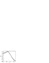
FIG. 8.: Specific heat coefficient C/T $\left(mJ/\left(gK^{2}\right)\right)$ versus T $\left(K\right)$ of $YBa_{2}Cu_{3}O_{7-\delta}$ ( sample YBCO3 [68]). The two arrows mark $T_{c}\approx 92.12K$ and $T_{P}\approx 91.98K$ , respectively.

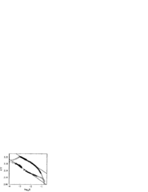
FIG. 9.: Specific heat coefficient C/T $\left(mJ/\left(gK^{2}\right)\right)$ versus log${}_{10}\left|t\right|$ for $YBa_{2}Cu_{3}O_{7-\delta}$ ( sample YBCO3 [68]) for $T_{c}=92.12K$.

A finite-size scaling analysis[14] reveals inhomogeneities with a characteristic length scale ranging from $300$ to $400$ A, in the YBa₂Cu₃O_7-δ samples YBCO3, UBC2 and UBC [68]. Note that recent measurements by a variety of techniques suggest that superconductivity is not homogeneous in cuprates[70, 71, 72].For this reason, deviations from $3D$-$XY$ critical behavior around $T_{p}$ do not signal the failure of $3D$-$XY$ universality, as previously claimed[68], but reflect a finite-size effect at work. Indeed from Fig.9 it is seen that the finite-size effect makes it impossible to enter the asymptotic critical regime. To set the scale we note that in the $\lambda$-transition of ⁴He the critical properties can be probed down to $\left|t\right|=10^{-9}$[73, 74]. In Fig.8 we marked the intermediate regime where consistency with the 3D-XY-critical behavior, ${C}/{T}=\widetilde{A}^{\pm}10^{-\alpha\log_{10}|t|}+\widetilde{B}^{\pm}$ for $\alpha=-0.013$ and $\widetilde{A}^{+}/\widetilde{A}^{-}=1.07$, can be observed in terms of full circles. The upper branch corresponds to $T<T_{c}$  and the lower one to $T>T_{c}$. The open circles closer to $T_{c}$ correspond to the finite-size affected region, while further away the temperature dependence of the background, usually attributed to phonons, becomes significant. Hence, due to the finite size effect and the temperature dependence of the background the intermediate regime is bounded by the temperature region where the data depicted in Fig. 9 fall nearly on straight lines. In this context it should be kept in mind that the effect of disorder and inhomogeneities is quite different. Since the critical exponent $\alpha$ of the specific heat is negative at the 3D-XY transition, Harris criterion implies that disorder is irrelevant so that the critical behavior will be that of the pure system [75]. To provide quantitative evidence for 3D-XY universality in this regime, we invoke the universal relations (10) and (18) to calculate $T_{c}$ from  the critical amplitudes of specific heat and penetration depth. Using $A^{+}=8.4\ 10^{20}$ $cm^{3}$, derived from the data shown in Fig.9 for sample YBCO3 with $T_{c}=92.12K$, $\lambda_{a,0}=1153A,\ \lambda_{b,0}=968A$ and $\ \lambda_{c,0}=8705A$  , derived from magnetic torque measurements on a sample with $T_{c}=91.7K$ [45], together with the universal numbers $A^{+}/A^{-}=1.07$ and $R^{-}\approx 0.59$[14], we obtain $T_{c}=88.2K$ . Hence, the universal 3D-XY-relations (10) and (18) are remarkably well satisfied.

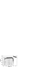
FIG. 10.: Scaling function $dG_{3}^{\pm}(\widetilde{z})/d\widetilde{z}$ derived from  the angular dependence of the magnetic torque for YBa₂Cu₃O_6.93, La_1.854Sr_0.146CuO₄, HgBa₂CuO_4.108, HgBa₂CuO_4.096, La_1.914Sr_0.086CuO₄ and La_1.920Sr_0.080CuO₄. Taken from [8].

Another difficulty in observing 3D-XY critical properties stems from the fact that most cuprates are highly anisotropic. A convenient measure of the anisotropy is $\gamma_{T_{c}}$ (Eq.(22)), which depends on the dopant concentration (see Figs.1 and 2). Although the strength of thermal fluctuations grows with increasing $\gamma$, they become essential 2D slightly away from $T_{c}$. Accordingly, the 3D-XY - critical regime shrinks and the corrections to scaling become significant. To document this point we depicted in Fig.10 estimates for the derivative of the universal scaling function $G_{3}^{\pm}(\widetilde{z})$ derived from magnetic torque measurements[8]. Even though the qualitative behavior is the same for all samples, the deviations increase with rising $\gamma_{T_{c}}$. This systematics cannot be attributed to the experimental uncertainties of about 40%. It is more likely that it reflects the reduction of the temperature regime where 3D-fluctuation dominates so that corrections to scaling become important[14]. In this view it is clear that due its moderate anisotropy[14, 45], optimally doped YBa₂Cu₃O_7-δ is particularly suited to observe and check the consistency with 3D-XY critical behavior. In contrast to this, in highly anisotropic cuprates like Bi₂Sr₂CaCu₂O_8-δ, it will be difficult to enter the regime where 3D fluctuations dominate [76]. Nevertheless, since the critical behavior of the charged fixed point is the only alternative left, it becomes clear that even the intermediate critical behavior of highly anisotropic cuprates like Bi₂Sr₂CaCu₂O_8-δ falls into the 3D-XY universality class. fluctuations grows with increasing $\gamma$, they become essential 2D slightly away from $T_{c}$. Accordingly, the 3D-XY - critical regime shrinks and the corrections to scaling become significant. To document this point we depicted in Fig.10 estimates for the derivative of the universal scaling function $G_{3}^{\pm}(\widetilde{z})$ derived from magnetic torque measurements[8]. Even though the qualitative behavior is the same for all samples, the deviations increase with rising $\gamma_{T_{c}}$. This systematics cannot be attributed to the experimental uncertainties of about 40%. It is more likely that it reflects the reduction of the temperature regime where 3D-fluctuation dominates so that corrections to scaling become important[14]. In this view it is clear that due its moderate anisotropy[14, 45], optimally doped YBa₂Cu₃O_7-δ is particularly suited to observe and check the consistency with 3D-XY critical behavior. In contrast to this, in highly anisotropic cuprates like Bi₂Sr₂CaCu₂O_8-δ, it will be difficult to enter the regime where 3D fluctuations dominate [76]. Nevertheless, since the critical behavior of the charged fixed point is the only alternative left, it becomes clear that even the intermediate critical behavior of highly anisotropic cuprates like Bi₂Sr₂CaCu₂O_8-δ falls into the 3D-XY universality class.

The melting transition of the vortex lattice was discovered in 1993 in Bi_2.15Sr_1.85CaCu₂O_8-δ using the $\mu$SR technique[77]. An anomaly attributed to this transition was observed in specific heat measurements of YBa₂Cu₃O_7-δ[78]. In Fig.11 we depicted the temperature dependence of the specific heat coefficient of an untwinned YBa₂Cu₃O_7-δ single crystal for various applied fields H$\|$c. Of particular interest in this context is the small anomaly below the main peak, marked by the strength of the applied field. It is attributed to the vortex melting transition. Evidence for the first order nature of the transition stems from magnetization measurements, revealing a jump at $H_{m}$[79], which signals the singularity in the scaling function $G_{3}^{\pm}(\widetilde{z})$ at $\widetilde{z}=\widetilde{z}_{m}$ (Eq.(26)).

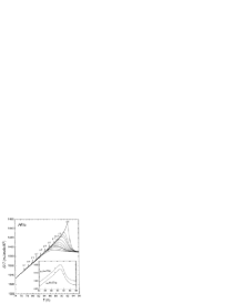
FIG. 11.: Temperature dependence of the specific heat coefficient for various applied magnetic fields $\left(H\|c\right)$ of an untwinned YBa₂Cu₃O_7-δ single crystal. The numbers on the top of the peak like features denote the applied field strength. The inset shows representative data for $H=1T$ $\left(H\|c\right)$ and $H=8T$ $\left(H\|(a,b)\right)$, data shifted vertically by 10 mJ/molK². Taken from [78].

Due to the first order nature of the transition, the correlation lengths remain bounded, so that the melting line $H_{cm}$ and the temperature $T_{P}$, where the broad peak in the specific heat coefficient adopts its maximum value, should scale according to Eqs.(30) and (31). A glance to Fig.12 shows that this behavior is experimentally well confirmed. Note that the variation of the amplitudes $A_{cm}$ and $A_{cp}$ is due to the doping dependence of $\xi_{a,0}\xi_{b,0}$ ( see Eqs.(30) and (31)). From Eq.(29) it is seen that the melting line also yields useful information on the anisotropy. As an example we consider the angular dependence in the (c,a) plane. Eq.(29) yields

$$H_{m}\left(\delta\right)=H_{m}\left(\delta=0\right)\gamma_{ca}\left(\sin^{2}\left(\delta\right)+\gamma_{ca}^{2}\cos^{2}\left(\delta\right)\right)^{-1/2},\text{ }\gamma_{ca}=\frac{\xi_{a}}{\xi_{c}},H_{m}\left(\delta=0\right)\propto\left(1-T/T_{c}\right)^{2\nu}.$$ (32)

FIG. 12.: Melting line $H_{c,m}$ and $H_{c,\max}$ versus $T-T_{c}$ for a $YBa_{2}CuO_{7-\delta}$ single crystal with $\delta=0$ ($\blacklozenge$), $\delta=0.03$ ($\blacktriangle$) and $\delta=0.053$ ($\bullet$) for H$\|$c. Taken from [80]. The curves correspond to $H_{cm}=A_{cm}\left(\frac{T_{c}-T}{T_{c}}\right)^{2\nu}$ and $H_{cp}=A_{cp}\left(\frac{T_{c}-T}{T_{c}}\right)^{2\nu}$ with$\ \nu=2/3$.

From Fig.13 it is seen that this behavior is well confirmed. In this context the question arises, whether or not phase coherence and with that superfluidity persists above the melting line. Recently, numerical simulations revealed that the vortex liquid is incoherent, i.e. phase coherence is destroyed in all directions, including the direction of the applied magnetic field, as soon as the vortex lattice melts[83, 84].

To summarize, there is considerable evidence that the intermediate finite temperature critical behavior of cuprate superconductors, when attained, is equivalent to that of superfluid helium. Moreover, we saw that finite size scaling is a powerful tool to identify and characterize inhomogeneities.

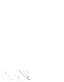
FIG. 13.: Left panel: Melting line for YBa₂Cu₃O_7-δ with $T_{c}=93.25K$ derived from field $\left(\bigcirc\right)$- and angular-dependent $\left(\square\right)$ torque curves. The solid line corresponds to $H_{m}\propto\left(1-T/T_{c}\right)^{2\nu}$ with $\nu=2/3$. Data taken from [81]. Right panel: Melting lines $H_{m}\left(\delta,T\right)$ for YBa₂Cu₃O_7-δ with $T_{c}=92K$, detected by a direct measurement of the entropy change. The symbols denote experimental data taken at different magnetic field orientations in the (c,a) plane, measured by the angle $\delta$[82]. The solid lines are Eq.(32) with $\gamma_{ca}=7.6$ and $\nu=2/3$.

III Quantum critical behavior and crossover phenomena

A Sketch of the scaling predictions

Given the empirical phase transition line $T_{c}\left(x\right)$ or surface $T_{c}\left(x,y\right)$ with critical endpoints or lines (see Figs.1 and 3) doping and substitution tuned quantum phase transitions can be expected. To invoke and sketch the scaling theory of quantum critical phenomena we define $\delta$, measuring the relative distance from quantum critical points, in terms of

$$\delta=\left\{\begin{array}[]{c}\ \ \ \ \ y=0\ \ \ \ \ \ \ \ \ \ \ \ \ \ \ \ \ \ \ \ \ :\delta=\left(x-x_{u}\right)/x_{u}\\ \ \ \ \ \ y=0\ \ \ \ \ \ \ \ \ \ \ \ \ \ \ \ \ \ \ \ \ \ :\delta=\left(x_{o}-x\right)/x_{o}\\ y\neq 0,\ \ x_{u}\leq x\leq x_{o}\ \ \ \ \ \ \ \ \ \ \ \ \ :\delta=\left(y_{c}\left(x\right)-y\right)/y_{c}\left(x\right)\end{array}\right..$$ (33)

At $T=0$ and close to quantum criticality one has two kind of correlation lengths[14, 47]. The usual spatial correlation length in direction $i$

$$\overline{\xi}_{i}^{-}=\overline{\xi}_{i,0}^{-}\delta^{-\overline{\nu}}$$ (34)

and the temporal one

$\displaystyle\overline{\xi}_{\tau}^{-}=\overline{\xi}_{\tau,0}^{-}\delta^{-\overline{\nu}_{\tau}},$

where the dynamic critical exponent is defined as the ratio

$$z=\frac{\overline{\nu}_{\tau}}{\overline{\nu}}.$$ (35)

The singular part of the free energy density adopts then the scaling form [14, 47, 15]

$$f_{s}\left(\delta,T\right)=\overline{Q}_{D}\left(\overline{\xi}_{\tau,0}^{-}\prod\limits_{i=1}^{D}\overline{\xi}_{i,0}^{-}\right)^{-1}\delta^{\overline{\nu}\left(D+z\right)}F_{D}\left(\overline{y}\right),\ \ \ \overline{y}=k_{B}T\overline{\xi}_{\tau}=k_{B}T\overline{\xi}_{\tau,0}\delta^{-z\overline{\nu}},$$ (36)

where $F_{D}\left(\overline{y}\right)$ with $F_{D}\left(\overline{y}=0\right)=1$ is a universal scaling function and $Q_{D}$ a universal constant. Another quantity of interest is the helicity modulus which adopts the scaling form [14, 15]

$$\Upsilon_{i}^{D}\left(\delta,T\right)=\overline{Q}_{D}\left(\overline{\xi}_{i,0}^{-}\right)^{2}\left(\overline{\xi}_{\tau,0}^{-}\prod\limits_{i=1}^{D}\overline{\xi}_{i,0}^{-}\right)^{-1}\delta^{\overline{\nu}\left(D-2+z\right)}Y_{D}\left(\overline{y}\right),$$ (37)

where $Y_{D}\left(\overline{y}\right)$ with $Y_{D}\left(y=0\right)=1$ is a universal scaling function of its argument. As a first application we consider a line of finite temperature transitions $T_{c}\left(\delta\right)$ ending at a quantum critical point at $T=0$ and $\delta=0$. The scaling forms then require that

$$k_{B}T_{c}=\frac{\overline{y}_{c}}{\overline{\xi}_{\tau,0}^{-}}\delta^{z\overline{\nu}},$$ (38)

where $y_{c}$ is the universal value of the scaling function argument at which the scaling functions exhibit a singularity at finite temperature. Combining Eqs.(37) and (38) we obtain in $D=2$

$$\frac{k_{B}T_{c}}{\Upsilon_{ab}^{D=2}\left(\delta,0\right)}=\overline{R}_{2},\ \ \ \overline{R}_{2}=\frac{\overline{y}_{c}}{Y_{2}\left(\overline{y}_{c}\right)\overline{Q}_{2}},$$ (39)

yielding the universal relation

$$T_{c}\lambda_{ab}^{2}\left(0\right)=\frac{\Phi_{0}^{2}\overline{R}_{2}}{16\pi^{3}k_{B}}d_{s},$$ (40)

between transition temperature and zero temperature in-plane penetration depth. $d_{s}$ denotes the thickness of the superconducting slab and $\overline{R}_{2}$ is a universal dimensionless constant. Analogously, in $D=3$ Eqs.(37) and (38) yield

$$\frac{k_{B}T_{c}}{\Upsilon_{ab}^{D=3}\left(\delta,0\right)}=\overline{R}_{3}\overline{\xi}_{c}^{-},\ \ \ \overline{R}_{3}=\frac{\overline{y}_{c}}{Y_{3}\left(\overline{y}_{c}\right)\overline{Q}_{3}},$$ (41)

so that $T_{c}$, $\lambda_{ab}^{2}\left(0\right)$, $\overline{\xi}_{c}^{-}$ and $\overline{\xi}_{ab}^{-}$ are related by

$$T_{c}\lambda_{ab}^{2}\left(0\right)=\frac{\Phi_{0}^{2}\ \overline{R}_{3}}{16\pi^{3}k_{B}}\overline{\xi}_{c}^{-}=\frac{\Phi_{0}^{2}\ \overline{R}_{3}}{16\pi^{3}k_{B}}\frac{\overline{\xi}_{ab}^{-}}{\gamma_{T=0}}.$$ (42)

This is just the quantum analogy of the universal finite temperature relation (23). When there is an anisotropy tuned 3D-2D crossover, where $\gamma_{T=0}\rightarrow\infty$, matching of Eqs.(40) and (42) requires that

$$\overline{R}_{3}\overline{\xi}_{c}^{-}=\overline{R}_{3}\frac{\overline{\xi}_{ab}^{-}}{\gamma_{T=0}}=\overline{R}_{2}d_{s}.$$ (43)

Noting then that the universal relation (42) applies close to both, the 2D-QSI and 3D-QSN transition it is expected to provide useful information on the correlation lengths ( $\overline{\xi}_{c}^{-}$, $\overline{\xi}_{ab}^{-}$), given experimental data for $T_{c}\lambda_{ab}^{2}\left(0\right)$ and $\gamma_{T=0}$.

Moreover, useful scaling relations for the specific heat coefficient $\gamma_{c}$ are readily derived from the singular part of the free energy density (36), namely:

$$\left.\gamma_{c}\right|_{T=0}=\left.\frac{c}{T}\right|_{T=0}=\left.\frac{\partial^{2}f_{s}}{\partial T^{2}}\right|_{T=0}\propto\delta^{\overline{\nu}\left(D-z\right)}\propto T_{c}^{\left(D-z\right)/z}\propto H_{c}^{\left(D-z\right)/2},$$ (44)

since $H_{c}$ scales as $H_{c}\propto\left(\overline{\xi}_{ab}^{-}\right)^{-2}$[14], when applied parallel to the c-axis, and

$$\left.\frac{d\gamma_{c}}{dT}\right|_{T=0}=\left.\frac{d}{dT}\left(\frac{c}{T}\right)\right|_{T=0}=\left.\frac{\partial^{3}f_{s}}{\partial T^{3}}\right|_{T=0}\propto\delta^{\overline{\nu}\left(D-2z\right)}\propto T_{c}^{\left(D-2z\right)/z}.$$ (45)

Finally, considering a 2D quantum critical points resulting from a 3D-2D crossover in the ground state, Eq.(43) implies that close to 2D quantum criticality the anisotropy diverges as

$$\gamma_{T=0}=\frac{\overline{\xi}_{ab}^{-}}{\overline{\xi}_{c}^{-}}=\frac{\overline{R}_{3}\overline{\xi}_{ab,0}^{-}}{\overline{R}_{2}d_{s}}\delta^{-\overline{\nu}}\propto T_{c}^{-1/z}.$$ (46)

Combining the scaling relations (38), (40), (43) and (46) a 2D quantum critical point resulting from a 3D-2D crossover is then characterized by

$$T_{c}\propto{\lambda_{ab}^{-2}}\left({0}\right)\propto n_{s}^{\square}\left(0\right)\propto\gamma_{T=0}^{-z}\propto\delta^{z\overline{\nu}},\ \ \ \left.\gamma_{c}\right|_{T=0}\propto T_{c}^{\left(2-z\right)/z}\propto H_{c}^{\left(2-z\right)/2}.$$ (47)

$n_{s}^{\square}\left(0\right)=\left(d_{s}/{\lambda_{ab}^{2}(0)}\right)$ denotes aerial superfluid density. In particular it relates the superconducting properties to the anisotropy parameter, fixing the dimensionality of the system. It reveals that an anisotropy driven 3D-2D crossover destroys superconductivity even in the ground state.

From Eq.(42), rewritten in the form

$$\overline{\xi}_{c}^{-}=\frac{16\pi^{3}k_{B}}{\Phi_{0}^{2}\ \overline{R}_{3}}T_{c}\lambda_{ab}^{2}\left(0\right),\ \ \overline{\xi}_{ab}^{-}=\frac{16\pi^{3}k_{B}}{\Phi_{0}^{2}\ \overline{R}_{3}}T_{c}\lambda_{ab}^{2}\left(0\right)\gamma_{T=0},$$ (48)

it is seen that $T_{c}\lambda_{ab}^{2}\left(0\right)$ and $T_{c}\lambda_{ab}^{2}\left(0\right)\gamma_{T=0}$ are appropriate indicators for the occurrence of quantum phase transitions. Close to 3D-QSN criticality $\overline{\xi}_{c}^{-}$ and $\overline{\xi}_{ab}^{-}$ diverge according  Eq.(34) as

$$\text{3D-QSN}:\overline{\xi}_{c}^{-}\propto\ \overline{\xi}_{ab}^{-}\propto\delta^{-\overline{\nu}}\propto T_{c}^{-1/z},$$ (49)

because $\gamma_{T=0}$ remains finite. This differs from the 2D-QSI transition, where according to relation (46)

$$\text{2D-QSI}:\overline{\xi}_{c}^{-}=\frac{\overline{R}_{2}}{\overline{R}_{3}}d_{s},\ \ \overline{\xi}_{ab}^{-}=\frac{\overline{R}_{2}}{\overline{R}_{3}}d_{s}\gamma_{T=0}\propto\delta^{-\overline{\nu}}\propto T_{c}^{-1/z},$$ (50)

applies. Here $\overline{\xi}_{c}^{-}$ tends to a finite value, proportional to the thickness $d_{s}$ of the sheets. valid for a 2D-XY - QSI transition. $\rho_{0}$ and $\rho_{0c}$ denote the residual and critical residual sheet resistivity.

Next we turn to the critical behavior of the conductivity. In the normal state and close to a 3D-XY critical point, the DC conductivities, parallel ($\sigma_{ab}^{DC}$) and perpendicular ($\sigma_{c}^{DC}$) to the layers, scale as[14]

$$\sigma_{ab}^{DC}\propto\frac{\xi_{\tau}}{\xi_{c}},\ \sigma_{c}^{DC}\propto\frac{\xi_{c}\xi_{\tau}}{\xi_{ab}^{2}},$$ (51)

where $\xi_{\tau}$ is the correlation length associated with the finite temperature critical dynamics. At $T_{c}$ the ratio is then simply given by the anisotropy

$$\frac{\sigma_{c}^{DC}}{\sigma_{ab}^{DC}}=\left(\frac{\xi_{c}}{\xi_{ab}}\right)^{2}=\left(\frac{1}{\gamma_{T_{c}}}\right)^{2}.$$ (52)

Approaching 2D-QSI criticality, the scaling relation (47) implies

$$\gamma_{T_{c}}=\gamma_{T_{c},0}\delta^{-\overline{\nu}}$$ (53)

Another essential property of this critical point is that for any finite $T_{c}$ the in-plane areal conductivity is always larger than[14, 47]

$$\sigma_{ab}^{DC}d_{s}=\sigma_{0}\frac{4e^{2}}{h}.$$ (54)

This follows from the fact that close to 2D-QSI the in-plane resistivity adopts the scaling form[14, 47]

$$\rho_{ab}=\frac{h}{4e^{2}\sigma_{0}}F\left(\overline{y}\right),\ \ \overline{y}=k_{B}T\overline{\xi}_{\tau}.$$ (55)

Thus, close to a 2D-QSI transition the normal state resistivity $\rho_{c}^{DC}\left(T_{c}^{+}\right)=1/\sigma_{c}^{DC}\left(T_{c}^{+}\right)$, evaluated close but slightly above $T_{c}$, is predicted to diverge as

$$\rho_{c}^{DC}\left(T_{c}^{+}\right)=\gamma_{T_{c}}^{2}\frac{h}{4e^{2}\sigma_{0}}=\gamma_{T_{c},0}^{2}\delta^{-2\overline{\nu}}\frac{h}{4e^{2}\sigma_{0}}.$$ (56)

$F\left(y\right)$ is a scaling function of its argument and $F\left(0\right)=1$. This behavior uncovers the 3D-2D crossover associated with the flow to 2D-QSI criticality in the normal state. To establish a relation between normal and superconducting properties, we express $\delta$ in terms of $\lambda_{c}\left(0\right)$. Using Eq.(47) we obtain

$$\lambda_{c}\left(0\right)=\Omega_{s}\left(\sigma_{c}^{DC}\left(T_{c}^{+}\right)\right)^{-\left(2+z\right)/4},\ \ \ \Omega_{s}=\gamma_{0,0}\lambda_{ab,0}\left(0\right)\left(\frac{4e^{2}\sigma_{0}}{h\gamma_{T_{c},0}^{2}}\right)^{\left(2+z\right)/4},$$ (57)

where

$$\gamma_{T}=\gamma_{T,0}\delta^{-\overline{\nu}},\ \ \lambda_{ab,0}\left(0\right)=\lambda_{ab,0}\left(0\right)\delta^{-z\overline{\nu}/2},$$ (58)

are the zero temperature critical amplitudes. The scaling relation (57) differs from the mean-field prediction for bulk superconductors in the dirty limit [85] and layered BCS superconductors, treated as weakly coupled Josephson junction[86, 87, 88]:

$$\lambda_{c}\left(0\right)=\Omega_{s}\left(\sigma_{c}^{DC}\left(T_{c}^{+}\right)\right)^{-1/2},$$ (59)

where

$$\Omega_{s}=\left(\frac{\hbar c^{2}}{4\pi^{2}\Delta\left(0\right)}\right)^{1/2},\text{ \ }\Delta\left(0\right)=1.76k_{B}T_{c}$$ (60)

and $\Delta\left(0\right)$ denotes the zero temperature energy gap.

Approaching 3D-QSN criticality, the finite temperature relations (51) and (52) still apply, but both, $\rho_{c}^{DC}$ and $\rho_{ab}^{DC}$ diverge at $T_{c}$, while the anisotropy $\gamma_{T_{c}}$ remains finite. For this reason $\xi_{\tau}$, the correlation length associated with the finite temperature critical dynamics, cannot be eliminated. Nevertheless, since $\xi_{\tau}$ scales as, $\xi_{\tau}\propto\xi_{ab}^{z_{cl}}$, where $z_{cl}$ is the critical exponent of the finite temperature dynamics, we obtain from Eq.(51) the relation

$$\sigma_{c}^{DC}\propto\frac{\xi_{c}\xi_{\tau}}{\xi_{ab}^{2}}\propto\frac{\xi_{\tau}}{\gamma_{T_{c}}\xi_{ab}}\propto\xi_{ab}^{z_{cl\ }-1}\propto\xi_{ab,0}^{z_{cl\ }-1}\left|t\right|^{-\nu\left(z_{cl\ }-1\right)},$$ (61)

valid close to 3D-XY critical points. Since close to a 3D-QSN criticality, the doping dependence of the finite temperature critical amplitude $\xi_{ab,0}$ is given by $\overline{\xi}_{ab}$ ( see Eqs.(23) and (42)), we finally obtain with $\ \lambda_{c}\left(0\right)\propto\delta^{-\frac{\overline{\nu}}{2}\left(1+z\right)}$ (Eq.(37)) the relationship between $\lambda_{c}\left(0\right)$ and $\sigma_{c}\left(T_{c}^{+}\right)$ the relationship

$$\lambda_{c}\left(0\right)\propto\left(\sigma_{c}\left(T_{c}^{+}\right)\right)^{\frac{1+z}{2\left(z_{cl}-1\right)}},$$ (62)

characterizing the flow to a 3D-QSN critical point in the $\left(\lambda_{c}\left(0\right),\sigma_{c}\left(T_{c}^{+}\right)\right)$ plane.

Noting that the in-plane resistivity tends close to 2D-QSI criticality to a fixed value (Eq.(55)), $\rho_{ab}$ can also be used as a parameter measuring the distance from the critical point. This is achieved by setting $y=k_{B}T\overline{\xi}_{\tau}\propto T\delta^{-z\overline{\nu}}\propto T\left(\left(\rho_{ab}^{0}-\rho_{ab}\right)/\rho_{ab}^{0}\right)^{-z\overline{\nu}}$. Given then a transition line $T_{c}\left(\delta\right)$ ending at the 2D-QSN critical point the scaling form (55) requires that

$$T_{c}\propto\left(\frac{\rho_{ab}^{0}-\rho_{ab}}{\rho_{ab}^{0}}\right)^{z\ \overline{\nu}},\ \rho_{ab}^{0}=\frac{h}{4e^{2}\sigma_{0}}$$ (63)

because the scaling function $F\left(y\right)$ exhibits a singularity at $y_{c}$, signaling the finite temperature transition line.

B Evidence for chemically doping tuned quantum phase transitions

The empirical correlations between $T_{c}$, dopant concentration $x$ and anisotropy $\gamma_{T}$ (Eqs.(1)-(3)) clearly point to the existence of quantum critical endpoints. A glance to Fig.2 shows, when $T_{c}$ vanishes in the underdoped limit, the anisotropy $\gamma_{T}$ tends to infinity. Accordingly a 2D-QSI transition is expected to occur. In the overdoped limit, $T_{c}$ vanishes again but the finite anisotropy implies a 3D-QSN transition. Since the aforementioned empirical correlations turned out to be remarkably generic (see Fig.2) they appear to reflect universal properties characterizing these quantum phase transitions. Indeed, the empirical correlation (1) points with the scaling law (38) to $\ z\overline{\nu}=1$ in both transitions. Moreover, the empirical relation between $T_{c}$ and $\gamma_{T}$ (3) implies according to the scaling law (46) a 2D-QSI transition with $\overline{\nu}=1$. Thus, the universality classes emerging from the empirical relations are characterized by the critical exponents:

$$\text{2D-QSI}:z=1,\ \overline{\nu}=1,$$ (64)

$$\text{3D-QSN}:z\overline{\nu}=1.$$ (65)

These 2D-QSI exponents are consistent with the theoretical prediction for a 2D disordered bosonic system with long-range Coulomb interaction. Here the loss of superfluidity is due to the localization of the pairs, which is ultimately responsible for the transition[59, 60]. A potential candidate for the 3D-QSN transition is the Ginzburg-Landau theory proposed by Herbut [61]. It describes a disordered d-wave superconductor to metal transition at weak coupling and is characterized by the critical exponents $z=2$ and $\overline{\nu}=1/2$, except in an exponentially narrow region. Since the resulting $z\overline{\nu}$ coincides with the value implied by the empirical correlation (1), one expects with the estimate (65),

$$\text{3D-QSN}:z=2,\ \overline{\nu}=1/2.$$ (66)

FIG. 14.: $T_{c}$ versus $\lambda_{ab}\left(T=0\right)^{-2}$ for La _2-xSr_xCuO₄ ( $\bigcirc$: [91], $\blacktriangle$: [10], $\Box$: [90]) YBa₂Cu₃O_7-δ ( $\bigtriangledown$: [92]) and Y_1-xPr_xBa₂Cu₃O_6.97 ($\otimes$: [93]). The dashed and solid lines correspond to Eq.67.

A characteristic property of a 2D-QSI transition, irrespective of the value of $z\overline{\nu}$, is the universal relation (40) between transition temperature and zero temperature penetration depth. An instructive example is the onset of superfluidity in ⁴He films adsorbed on disordered substrates, where the linear relationship between $T_{c}$ and aerial superfluid density $n_{s}^{\square}\left(0\right)\propto d_{s}/{\lambda_{ab}^{2}}\left({0}\right)$ is well confirmed[89]. In cuprates, a nearly linear relationship between $T_{c}$ and $\lambda_{ab}\left(T=0\right)^{-2}$ has been established some time ago by Uemura et al. [90]. In the present context, it is not strictly universal, because $d_{s}$, the thickness of the independent slabs, is known to adopt family dependent values[14, 94]. This fact can be anticipated from Fig.14, showing experimental data for $T_{c}$ versus $1/\lambda_{ab}^{2}\left(T=0\right)$ of  La_2-xSr_xCuO₄ [10, 90, 91], YBa₂Cu₃O_7-δ [92] and Y_1-xPr_xBa₂Cu₃O_6.97 [93]. With $T_{c}$ in K and $\lambda_{ab}(T=0)$ in A, the dashed and solid straight lines correspond to

$$T_{c}\approx\frac{3.2\ 10^{8}}{\lambda_{ab}^{2}\left(T=0\right)},\ \frac{2.5\ 10^{8}}{\lambda_{ab}^{2}\left(T=0\right)}.$$ (67)

Invoking then the universal relation (40) we obtain the estimate,

$$\frac{d_{s}\left(\text{YBa}_{2}\text{Cu}_{3}\text{O}_{7-\delta}\right)}{d_{s}\left(\text{La}_{2-x}\text{Sr}_{x}\text{CuO}_{4}\right)}\approx\frac{3.2}{2.5}\approx 1.3,$$ (68)

which is consistent with , $d_{s}\left(\text{YBa}_{2}\text{Cu}_{3}\text{O}_{7-\delta}\right)\ /\ d_{s}\left(\text{La}_{2-x}\text{Sr}_{x}\text{CuO}_{4}\right)\approx 10.1\ A/7.6\ A\approx 1.33$, derived from the thickness tuned QSI transition and the crossing point phenomenon, respectively [14, 94]. Consequently, $dT_{c}/d(1/\lambda_{\|}^{2}(T=0))$ is not strictly universal. Nevertheless, due to the small variations of $d_{s}$ within a family of cuprates it adopts there a nearly unique value. For this reason the empirical proportionality of $T_{c}$ and $\lambda_{ab}\left(T=0\right)^{-2}$ for underdoped members of a given family confirms the flow to 2D-QSI criticality.

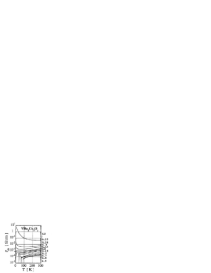
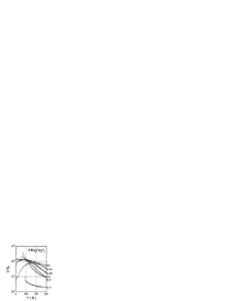
FIG. 15.: Left panel: Temperature dependence of the in-plane resistivity $\rho_{ab}$ of YBa₂Cu₃O_y at various dopant concentrations $y$. Taken from Semba and Matsuda[95]. The threshold resistivity is indicated by an arrow. Right panel: $\rho_{c}/\rho_{ab}$ versus $T$ of underdoped YBa₂Cu₃O_y. Taken from Semba and Matsuda [95].

Next we turn to the behavior of the resistivity close to 2D-QSI criticality. In Fig.15 we displayed the data of Semba and Matsuda [95] for the temperature dependence of the in-plane resistivity $\rho_{ab}$ of YBa₂Cu₃O_y at various dopant concentrations $y$. Below $y\approx 6.3$ the resistivity increases with decreasing temperature, signaling the onset of insulating behavior in the zero temperature limit. Above $y\approx 6.3$ and as the temperature is reduced, the resistivity drops rapidly and vanishes at and below $T_{c}$. Thus, for $y\gtrsim 6.3$ there is a superconducting phase and the 2D-QSI-transition occurs at $y\approx 6.3$. Moreover, the temperature dependence of $\rho_{c}/\rho_{ab}$, depicted in Fig.15, is in accord with the scaling relations (38) and (52), yielding $\rho_{c}/\rho_{ab}=\gamma_{T_{c}}^{2}\propto\delta^{-2\overline{\nu}}\propto T_{c}^{2/z}$. Indeed, the anisotropy increases by approaching the 2D-QSI transition. In contrast, near the 2D-QSI transition ($y\approx 6.3$), there is a finite threshold in-plane resistivity $\rho_{ab}^{th}$ $\approx 0.8m\Omega cm$ (see Fig.15). According to the scaling relation (54) this is a characteristic feature of a 2D-QSI transition. For $d_{s}\approx 11.8A$ and $\sigma_{0}\approx 1$ this leads to the sheet resistance $\rho_{ab}^{th}/d_{s}\approx h/\left(4e^{2}\right)\approx 6.5\ \ k\Omega$. Since $\rho_{c}\propto\gamma^{2}\rho_{ab}$ and $\rho_{ab}^{th}\rightarrow d_{s}h/\left(4e^{2}\right)$ it also becomes evident that the rise of $\rho_{c}$ for $T>T_{c}$ simply reflects the increasing anisotropy and with that the flow to 2D-QSI criticality. Together with the doping dependence of $\gamma_{Tc}$ (see Figs.1 and 2), these features clearly confirm the occurrence of a 2D-QSI transition.

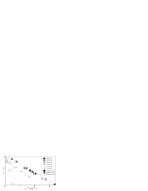
FIG. 16.: Residual in-plane resistance versus normalized critical temperature for Zn-substituted La_2-xSr_xCuO₄ and YBa₂Cu₃O_7-δ. $T_{c0}$ is the transition temperature of the Zn free compound. Taken from Fukuzumi et al. [4].

According to Eqs.(40) and (63)a 2D-QSI-transition is also characterized by the scaling relation

$$k_{B}T_{c}=c\left(\frac{\rho_{0c}-\rho_{0}}{\rho_{0c}}\right)^{z\ \overline{\nu}}={\frac{\Phi_{0}^{2}}{16\pi^{3}\overline{Q}_{2}}}{\frac{d_{s}}{\lambda_{ab}^{2}(T=0)},}$$ (69)

where $\rho_{0}$ and $\rho_{0c}$ denote the residual and critical residual sheet resistivity, respectively. This prediction is well confirmed by the data of Fukuzumi et al. for Zn-substituted La_2-xSr_xCuO₄ and YBa₂Cu₃O_7-δ [4] displayed in Fig.16. Approaching the underdoped limit the data merge on a straight line. With the scaling relation (69) this points to $z\overline{\nu}=1$ consistent with the value emerging from the empirical correlations (Eq.(64)).

FIG. 17.: Oxygen isotope effect for underdoped La_2-xSr_xCuO₄ in terms of $\ -T_{c}/\Delta T_{c}$  versus $\ -\left(1/{\lambda_{ab}^{2}(0)}\right)/\Delta\left(1/{\lambda_{ab}^{2}(0)}\right)$. The solid line marks the critical behavior at the 2D-QSI transition (Eq.(70)), while the dashed curves indicates the crossover to criticality. Experimental data taken from: $\bullet$ [96], $\blacksquare$ [97] and $\blacktriangle$ [98].

Next we turn to the isotope effect. Since universal relations like (18), (23) and (40) should apply irrespective of the doping and substitution level, the isotope effects on the quantities involved, are not independent. As an example we consider the universal relation (40), predicting that close to the 2D-QSI transition the isotope effect on transition temperature and zero temperature in-plane penetration depth are related by

$$\frac{\Delta T_{c}}{T_{c}}=\frac{\Delta\left(1/\lambda_{ab}^{2}\left(0\right)\right)}{1/\lambda_{ab}^{2}\left(0\right)},$$ (70)

where $\Delta\left(B\right)$ denotes the shift of $B$ upon isotope substitution. Although the available experimental data on identical samples are rather sparse, the results shown in Fig.17 for the oxygen isotope effect in La_2-xSr_xCu_1-xO₄ [96, 97] and Y${}_{1-x}\Pr_{x}$Ba₂Cu₃O₇ clearly reveal the crossover to the asymptotic 2D-QSI behavior marked by the straight line. An essential result is that the flow to 2D-QSI criticality implies that the isotope coefficients

$$\beta_{T_{c}}=-\frac{m}{T_{c}}\frac{\Delta T_{c}}{\Delta m},\ \ \beta_{\lambda}=-\frac{m}{T_{c}}\frac{\Delta\left(1/\lambda_{ab}^{2}\left(0\right)\right)}{\Delta m},$$ (71)

diverge. Some insight is obtained by noting that in the doping regime of interest, isotope substitution does not affect the dopant and substitution concentrations. [96]. In contrast it lowers the transition temperature and shifts the underdoped limit $x_{u}$[41, 99]. From the relation $T_{c}=a\ \delta^{z\overline{\nu}}$ (Eq.(38)), yielding

$$\frac{\Delta T_{c}}{T_{c}}=-\frac{z\overline{\nu}}{x/x_{u}-1}\frac{\Delta x_{u}}{x_{u}},$$ (72)

we obtain for the isotope coefficient the expression

$$\beta_{T_{c}}=\frac{1}{\overline{r}}\left(\frac{T_{c}\left(x_{m}\right)}{T_{c}}\right)^{1/z\overline{\nu}},\ \ \frac{1}{\overline{r}}=z\overline{\nu}\frac{m}{\Delta m}\frac{\Delta x_{u}}{x_{u}}\left(\frac{a}{T_{c}\left(x_{m}\right)}\right)^{1/z\overline{\nu}},$$ (73)

applicable close to the 2D-QSI transition. Here we rescaled $T_{c}$ by $T_{c}\left(x_{m}\right)$, the transition temperature at optimum doping, to reduce variations of $T_{c}$ between different materials [41]. In Fig.18 we show the experimental data for Y${}_{1-x}\Pr_{x}$Ba₂Cu₃O₇ [99], La_1.85Sr_0.15Cu_1-xNi_xO₄ [100] and YBa_2-xLa_xCu₃O₇ [101] in terms of $1/\beta_{T_{c}}$ versus $T_{c}/T\left(x_{m}\right)$. As predicted by Eq.(73), approaching the 2D-QSI transition $T_{c}/T_{c}\left(x_{m}\right)=0$, the data collapse on a straight line, pointing again to $z\overline{\nu}\approx 1$(Eq.(64)). Accordingly, the strong doping dependence of the isotope coefficients of transition temperature and zero temperature in-plane penetration depth in underdoped cuprates follows naturally from the doping tuned 3D-2D crossover and the associated 2D-QSI transition in the underdoped limit. One might hope that this novel point of view about the isotope effects in cuprate superconductors [102] will stimulate further experimental work to obtain new data to confirm or refute these predictions.

FIG. 18.: Inverse isotope coefficient $1/\beta_{T_{c}}$ versus $T_{c}/T_{c}^{m}$ for Y${}_{1-x}\Pr_{x}$Ba₂Cu₃O₇ [99], La_1.85Sr_0.15Cu_1-xNi_xO₄ [100] and YBa_2-xLa_xCu₃O₇ [101]. The straight line corresponds to $1/\beta_{T_{c}}=$ $\overline{r}\ T_{c}/T_{c}^{m}$ (Eq.(73)) with $z\overline{\nu}=1$ and $\overline{r}=6$.

A property suited to shed light on the critical behavior of both, the 2D-QSI and 3D-QSN transition is the magnetic field dependence of the specific heat coefficient in the limit of  zero temperature. From the scaling relation $\left.\gamma_{c}\right|_{T=0}\propto H_{c}^{\left(D-z\right)/2}$ (Eq.(44)) it is seen that for both transition $\left.\gamma_{c}\right|_{T=0}\propto H_{c}^{1/2}$ holds, provided that $z=1$ and $z=2$ at 2D-QSI and 3D-QSN criticality, respectively. The experimental data displayed in Fig.19 shows that in La_2-xSr_xCuO₄ $\left(D-z\right)/2=1/2$ holds irrespective of the doping level. Thus these data provide rather unambiguous evidenced for a 2D-QSI transition with $z=1$ and a 3D-QSN criticality with $z=2$. This implies that $\left.\gamma_{c}\right|_{T=0}\propto H_{c}^{1/2}$ is not a characteristic feature of d-wave pairing, as proposed by Volovik[104], Won and Maki[105].

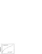
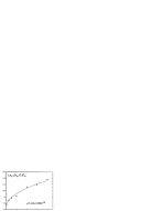
FIG. 19.: Magnetic field dependence of the specific heat coefficient at zero temperature $\left.\gamma_{c}\right|_{T=0}$ for La_2-xSr_xCuO₄ at x=0.1, 0.16 and 0.22. Taken from Chen et al.[103].

The above comparison with experiment provides rather clear evidence for the occurrence of a 2D-QSI transition with $z=1$ and $\overline{\nu}=1$ in the underdoped and a 3D-QSI critical point $z=2$ and $\overline{\nu}=1/2$ in the overdoped limit. Next, to substantiate this scenario further, we consider the crossover between these quantum critical points. Noting that $1/\lambda_{ab}^{2}\left(0\right)$ scales close to these critical points as (Eq.(37))

$$\frac{1}{\lambda_{ab}^{2}\left(0\right)}\propto\Upsilon_{ab}^{D}\left(0\right)\propto\delta^{\overline{\nu}\left(\left(D-2+z\right)\right)},$$ (74)

we invoke

$$\lambda_{ab}^{2}\left(0\right)=\frac{a_{\lambda}}{x-x_{u}}+\frac{b_{\lambda}}{\left(x_{o}-x\right)^{3/2}},$$ (75)

to interpolate between the 2D-QSI and 3D-QSN transition. A fit to the experimental data of La_2-xSr_xCuO₄, yielding the parameters

$$a_{\lambda}=5.42\ 10^{5}\ A^{2},\ \ b_{\lambda}=6.9\ 10^{3}\ A^{2},$$ (76)

is shown Fig.20.

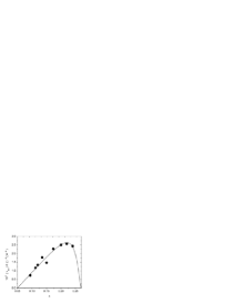
FIG. 20.: $1/\lambda_{ab}^{2}\left(0\right)$ versus $x$ for La_2-xSr_xCuO₄. $\bullet$: experimental data taken from [10, 90]. The solid curve is a fit to Eq.(75) with the parameters listed in Eq.(76). It indicates the crossover from a 2D-QSI transition with $z=1$ and $\overline{\nu}=1$ to a 3D-QSN criticality with $z=2$ and $\overline{\nu}=1/2$.

FIG. 21.: (a) $T_{c}\lambda_{ab}^{2}\left(0\right)$ versus $x$ for for La_2-xSr_xCuO₄. $\bullet$: taken from [10] and [90]. The solid line is Eqs.(1) and (75) with $T_{c}\left(x_{m}\right)=39.8K$ and the parameters listed in Eq.(76). Note that close to the 2D-QSI and 3D-QSN transition $T_{c}\lambda_{ab}^{2}\left(0\right)\propto\overline{\xi}_{c}$. (b) $T_{c}\lambda_{ab}^{-2}\left(0\right)\gamma_{T=0}$ versus $x$ for La_2-xSr_xCuO₄. $\bullet$ : $T_{c}$ and $\lambda_{ab}^{-2}\left(0\right)$ taken from [10, 90] and $\gamma_{T=0}$ from Eq.(2) with $\gamma_{T=0,0}=2$. Note that $T_{c}\lambda_{ab}^{-2}\left(0\right)\gamma_{T=0}\propto\overline{\xi}_{ab}$(48). The solid curve indicates the crossover from 2D-QSI $\left(z=1,\ \overline{\nu}=1\right)$ to 3D-QSN $\left(z=2,\ \overline{\nu}=1/2\right)$ criticality according to Eqs.(1), (2), (74) and (75).

It is remarkable that this simple interpolation scheme, reducing in the under- and overdoped limit to the expected asymptotic behavior, describes the data so well. Due to this agreement, this interpolation function provides in conjunction with the empirical law for $T_{c}\left(x\right)$ (Eq.(1)), a realistic description of the doping dependence of the zero temperature out-of-plane correlation length $\overline{\xi}_{c}$, given by Eq.(48), yielding $\overline{\xi}_{c}^{-}\propto T_{c}\lambda_{ab}^{2}\left(0\right)$, close to 2D-QSI and 3D-QSN criticality. The doping dependence of $T_{c}\lambda_{ab}^{2}\left(0\right)$ is displayed in Fig.21 for La_2-xSr_xCuO₄. Since $T_{c}\propto d_{s}/\lambda_{ab}^{2}\left(0\right)$ holds in the underdoped limit (see Eq.(40) and Fig.14), it is clear that $T_{c}\lambda_{ab}^{2}\left(0\right)$ tends to a constant value, proportional to $d_{s}$, the thickness of the independent sheets. Since initially $d/dx\left(T_{c}\lambda_{ab}^{2}\left(0\right)\right)\approx-T_{c}\left(x_{m}\right)a_{\lambda}x_{o}$, the linear decrease simply reflects the parabolic form of the empirical law (1). Finally, the upturn close to the overdoped limit, a regime which experimentally has not yet been attained, signals the 3D-QSN transition, where $\overline{\xi}_{c}\propto T_{c}\lambda_{ab}^{2}\left(0\right)$ diverges. In this context it is also instructive to consider the zero temperature in-plane correlation length. By definition it diverges at a 2D and 3D quantum phase transition. According to the scaling relation (48) it can be measured in terms of $\overline{\xi}_{ab}\propto T_{c}\lambda_{ab}^{2}\left(0\right)\gamma_{T=0}$. In Fig.21 we displayed the experimental data for $\overline{\xi}_{ab}\propto T_{c}\lambda_{ab}^{2}\left(0\right)\gamma_{T=0}$ versus $x$. For comparison we included the behavior resulting from Eqs.(1), (2),(74) and (75) in terms of the solid curve. While the rise of $\overline{\xi}_{ab}$ in the underdoped regime, signaling the occurrence of a 2D-QSI transition, is well confirmed, it does not extend sufficiently close to the overdoped limit to detect 3D-QSN criticality. From Fig.22, showing the doping dependence of the $T$-linear term of the specific heat coefficient of La_2-xSr_xCuO₄, it is seen that this quantity tends to a finite value in the underdoped limit and increases in the overdoped regime. This behavior is fully consistent with the scaling relation $\left.d\gamma_{c}/dT\right|_{T=0}\propto\delta^{\overline{\nu}\left(D-2z\right)}$ (Eq.(45)). Indeed at 2D-QSI criticality with $z=1$, $\left.d\gamma_{c}/dT\right|_{T=0}$ tends to a constant value and diverges close to the 3D-QSN critical point for $z>3/2$. Unfortunately, the data does not extend sufficiently close to the overdoped limit to provide reliable estimates of the exponent combination $\overline{\nu}\left(3-2z\right)$.

FIG. 22.: $\left.T_{c}d\gamma_{c}/dT\right|_{T=0}$ versus $x$ for La_2-xSr_xCuO₄.Data taken from [16] and [106].

Provided that the linear T-term of $1/\lambda_{ab}^{2}\left(T\right)$ in the zero temperature limit exists, the scaling relations (37) and (38) yield close to quantum criticality the universal relation

$$T_{c}\left.\frac{d}{dT}\left(\frac{\lambda_{i}(0)}{\lambda_{i}(T)}\right)^{2}\right|_{T=0}=\overline{y}_{c}\left.\frac{d{Y}_{D}}{d\overline{y}}\right|_{\overline{y}=0},$$ (77)

where D=2 and D=3 for the 2D-QSI and 3D-QSN transition, respectively. In Table I we collected additional estimates for various cuprates and doping levels. The rise of   the magnitude of $T_{c}\left.d/dT\left(\lambda_{ab}(\delta,0)/\lambda_{i}(\delta,T)\right)^{2}\right|_{T=0}$ with increasing doping level reflects the 2D-3D-crossover in the scaling function $Y_{D}$. Noting that most compounds are close to optimum doping it is not surprising that the listed values scatter around -0.61, the value of nearly optimally doped La_2-xSr_xCuO₄.

	$\lambda_{ab}\left(0\right)$ (A)	Tc (K)	$T_{c}\left.\frac{d}{dT}\left(\frac{\lambda_{i}(\delta,0)}{\lambda_{i}(\delta,T)}\right)^{2}\right|_{T=0}$
HgBa2Ca2Cu3O8+δ	1770	135	-0.59
HgBa2CuO4+δ	1710	93	-0.65
La1.9Sr0.1CuO4	2800	30	-0.49
La1.85Sr0.15CuO4	2600	39	-0.61
La1.8Sr0.2CuO4	1970	35	-0.72
La1.78Sr0.22CuO4	1930	27.5	-0.72
La1.76Sr0.24CuO4	1940	19	-0.94
Bi2Sr2CaCu2O8+δ	2600	91	-0.61
Y0.94Ca0.06Ba2Cu4O8	1361	88	-0.51
YBa2Cu4O8	1383	81	-0.58
YBa1.925La0.075Cu4O8	1521	74	-0.61
YBa1.9La0.1Cu4O8	1593	72	-0.63

Table I: Estimates for $T_{c}\left.d/dT\left(\lambda_{ab}\left(0\right)/\lambda_{ab}\left(T\right)\right)^{2}\right|_{T=0}$ derived from the experimental data of: slightly underdoped HgBa₂Ca₂Cu₃O_8+δ, slightly overdoped HgBa₂CuO_4+δ [107], under-, optimally- and over-doped La_2-xSr_xCuO₄ [10], Bi₂Sr₂CaCu₂O_8+δ [108], Y_0.94Ca_0.6Ba₂Cu₄O₈, YBa₂Cu₄O₈, Y_1.925La_0.075Cu₄O₈ and Y_1.9La_0.1Cu₄O₈ [109].

Before turning to the substitution tuned quantum transitions it is useful to express the doping dependence in the interpolation formula (75) in terms of the transition temperature. This is achieved by invoking the empirical correlation 1 between $T_{c}$ and doping concentration $x$ . In Fig.23 we displayed the resulting Uemura plot, $T_{c}$ versus $1/\lambda_{ab}^{2}\left(0\right)$ for La_2-xSr_xCuO₄ in terms of the solid and dashed curves, resembling the outline of a fly’s wing. The solid curve marks the flow from $T_{c}\left(x_{m}\right)$ to the 2D-QSI critical point and the dashed one the flow to 3D-QSN criticality. The dotted line indicates the universal 2D-behavior (Eqs.(40)) and (67)). For comparison we included the experimental data of Panagopoulos et al.[10] and Uemura et al.[90]. Although the data does not attain the respective critical regimes, together with the theoretical curves, they provide a generic perspective of the flow to 2D-QSI and 3D-QSN criticality. Indeed convincing evidence for these flows emerges from the $\mu$SR data displayed in Fig.24 for Y_0.8Ca_0.2Ba₂(Cu_1-yZn_y)O_7-δ (Y_0.8Ca_0.2-123), Tl_0.5-yPb_0.5+ySr₂Ca_1-xY_xCu₂O₇ (Tl-1212) [110] and TlBa₂CuO${}_{6+\delta}\ \left(\text{Tl-2201}\right)$ [111]. In analogy to Fig.23, the solid curves mark the flow from $T_{c}\left(x_{m}\right)$ to the 2D-QSI critical point and the dashed ones the approach to 3D-QSN criticality.

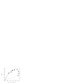
FIG. 23.: $T_{c}$ versus $1/\lambda_{ab}^{2}\left(0\right)$ for La_2-xSr_xCuO₄. $\bullet$: experimental data taken from [10, 90]. The solid and dashed curves result from the empirical law (1) and the interpolation function (75) with $T_{c}\left(x_{m}\right)$=39.8 K and the parameters listed in Eq.(76). The solid line indicates the flow from optimum doping to 2D-QSI criticality and the dashed one to the 3D-QSN critical point.

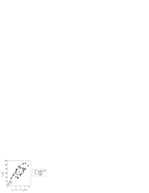
FIG. 24.: $T_{c}$ versus $\sigma_{0}\propto\lambda_{ab}^{-2}\left(0\right)$ for Y_0.8Ca_0.2Ba₂(Cu_1-yZn_y)O_7-δ (Y_0.8Ca_0.2-123), Tl_0.5-yPb_0.5+ySr₂Ca_1-xY_xCu₂O₇ (Tl-1212)[110] and TlBa₂CuO_6+δ (Tl-2201) [111]. The solid and dashed curves result from the empirical law (1) and the interpolation function (75). The solid curves indicate the flow from optimum doping to 2D-QSI criticality and the dashed ones to the 3D-QSN critical point.

A generic flow to the 2D-QSI critical point also emerges from the plot $\lambda_{c}\left(0\right)$ versus $\sigma_{c}\left(T_{c}^{+}\right)$ displayed in Fig.25 for YBa₂Cu₃O_7-δ, La_2-xSr_xCuO₄ and Bi₂Sr₂CaCu₂O_y at various doping levels. An empirical, nearly linear, correlation between these quantities has been proposed by Basov et al[112]. From the scaling relation (57) it is seen that the systematic rise of $\lambda_{c}\left(0\right)$ with decreasing $\sigma_{c}\left(T_{c}^{+}\right)$, tuned by decreasing dopant concentration and the associated rise of the anisotropy $\gamma_{T}$, reflects again the flow to 3D-QSI criticality. The straight line marks the asymptotic behavior La_2-xSr_xCuO₄ for $z=1$ and $\Omega_{s}\approx 24\mu m\left(\Omega cm\right)^{3/4}$. Since $\Omega_{s}$ depends on the critical amplitudes $\gamma_{0,0}$, $\lambda_{ab,0}\left(0\right)$, $\gamma_{T_{c},0}$ and the thickness $d_{s}$ (Eqs.(57) and (58)), its value is unique within a family of cuprates. $\Omega_{s}\approx 24\mu m\left(\Omega cm\right)^{3/4}$ follows from $\gamma_{0,0}\approx 1.63$, $\gamma_{T_{c},0}\approx 2$ (see Fig.1), $d_{s}\approx 6.6\ A$, $\sigma_{0}\approx 1$ and $\lambda_{ab,0}\left(0\right)\approx 736\ A$ (Eq.(76). Although the experimental data is still quite far from the underdoped limit, the flow to 2D-QSI criticality with family dependent values of $\Omega_{s}$ can be anticipated. This differs from the mean-field prediction for bulk superconductors in the dirty limit and layered BCS superconductors, treated as weakly coupled Josephson junctions (see Eqs.(59) and (60)) where $\Omega_{s}\propto T_{c}^{-1/2}$. Moreover, as the optimally doped and underdoped regimes are approached, systematic deviations from the straight line behavior appear, indicating the flow to 3D-QSN-criticality (Eq.(62)).

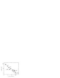
FIG. 25.: $\lambda_{c}\left(0\right)$ versus $\sigma_{c}\left(T_{c}^{+}\right)$ for YBa₂Cu₃O_7-δ ($\blacktriangle$), La_2-xSr_xCuO₄ ($\bullet$ )[113] and Bi₂Sr₂CaCu₂O_y ($\blacksquare$)[114]. The straight line is Eq.(57) with $z=1$ and $\Omega_{s}\approx 24\mu m\left(\Omega cm\right)^{3/4}$ , the estimate for La_2-xSr_xCuO₄.

According to the empirical correlation between $T_{c}$ and anisotropy $\gamma_{T}$ (see Eq.(3) and Fig.2), the initial value of the dopant concentration determines whether the flow leads to 2D-QSI or 3D-QSN criticality. For initially underdoped cuprates, the rise of $\gamma_{T}$ , tuned by the doping induced reduction of $T_{c}$, directs the flow to 2D-QSI criticality. Conversely, in initially overdoped cuprates, the fall of $\gamma_{T}$  to a finite value drives the flow to the 3D-QSN critical point. As the nature of the quantum phase transitions is concerned we have seen that the 2D-QSI transition has a rather wide and experimentally accessible critical region. For this reason we observed considerable and consistent evidence that it falls into the same universality class as the onset of superfluidity in ⁴He films in disordered media, corrected for the long-rangeness of the Coulomb interaction. The resulting critical exponents, $z=1$ and $\overline{\nu}\approx 1$, are also consistent with the empirical relations (Eqs.(1), (2) and (3)) and the observed temperature and magnetic field dependence of the specific heat coefficient in the limit of zero temperature. These properties also point to a 3D-QSN transition with $z=2$ and $\overline{\nu}\approx 1/2$, describing a d-wave superconductor to disordered metal transition at weak coupling. Here the disorder destroys superconductivity, while at the 2D-QSI transition it localizes the pairs and with that destroys superfluidity. Due to the existence of the 2D-QSI and 3D-QSN critical points, the detection of finite temperature 3D-XY critical behavior will be hampered by the associated crossovers which reduce the temperature regime where thermal 3D-XY fluctuations dominate. In any case, our analysis clearly revealed that the universality of the empirical correlations reflect the flow to 2D-QSI and 3D-QSN criticality. Moreover, the doping tuned superconductivity in bulk cuprate superconductors turned out to be a genuine 3D phenomenon, where the interplay of anisotropy and superconductivity destroys the latter in the 2D limit.

C Evidence for substitution tuned quantum phase transitions

It is well established, both experimentally and theoretically, that in conventional superconductors (e.g., A15 compounds or the Chevrel phases) the presence of magnetic impurities depresses the superconducting transition temperature more efficiently than does the introduction of nonmagnetic ions [115], and this has been ascribed to the breaking of pairs by the magnetic impurities. To determine wether the cuprates behave similarly with respect to magnetic impurities, extensive studies involving the substitution for Cu by other 3d metals have been performed [20, 19]. A result common to all these studies is that $\ T_{c}$ is depressed in the same manner, independent of wether the substituent is magnetic or nonmagnetic, and in contrast to that observed in conventional superconductors.

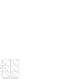
FIG. 26.: Variation of $T_{c}$ with substitution for La_1.95Sr_0.15Cu_1-yA_yO₄ ( A=Fe, Cu, Ni, Zn, Ga and Al ). Taken from Xiao et al. [19]

To illustrate this point we depicted in Fig.26, the variation of $T_{c}$ with substitution for La_1.95Sr_0.15Cu_1-yA_yO₄ (A=Fe, Cu, Ni, Zn, Ga and Al) [19]. $T_{c}$ is seen to vanish at a critical substitution concentration $y_{c}$, where a quantum phase transition occurs. The experimental data for La_2-xSr_xCu_1-yZn_yO₄, Y_0.8Ca_0.2Ba₂Cu_3-3yZn_3yO_7-δ [116] and Bi₂Sr₂CaCu_2-2yCo_2yO_8+δ [117] shows that this behavior is not restricted to optimum doping. Thus $T_{c}$ dependence on both, the dopant ($x$) and substitution concentration ($y$). Fig.3 shows the resulting ($T_{c},x,y$) diagram for La_2-xSr_xCu_1-yZn_yO₄. The blue curve, $y_{c}\left(x\right)$, is a line of quantum phase transitions. At the corresponding critical endpoints the system undergoes a 2D-QSI and 3D-QSN transition. Along the path marked by the green arrow, a QSI and QSN transition is expected to occur. The pink arrow indicates the crossover from insulating to metallic behavior.

FIG. 27.: Temperature dependence of the resistivity for La_2-xSr_xCu_1-yZn_yO₄ at $y_{c}\left(x\right)$. Taken from Momono et al. [16].

This scenario, emerging from the temperature dependence of the resistivity of La_2-xSr_xCu_1-yZn_yO₄[16], is shown in Fig.27. Along the phase transition line $y_{c}\left(x\right)$ superconductivity disappears and for $x\gtrsim 0.16$  metallic behavior sets in, while for $x\lesssim 0.16$ the resistivity exhibits insulating behavior at low temperatures. For fixed $x$ and close to $y_{c}\left(x\right)$, $T_{c}$ scales according to Eqs.(33)  and (38) as

$$T_{c}\left(y\right)\propto\ \left(1-\frac{y}{y_{c}\left(x\right)}\right)^{z\overline{\nu}}.$$ (78)

Since $z\overline{\nu}=1$ is expected to hold in both, the doping tuned 2D-QSI and 3D-QSN transition (Eqs.(64) and (66)), this combination should hold along the entire line $y_{c}\left(x\right)$. Although the data shown in Fig.26 is remarkably consistent with $z\overline{\nu}=1$ it remains to be understood, why the linear relationship applies almost over the entire substitution regime. Close to the 2D-QSI and 3D-QSN transitions, the singular part of the free energy density scales in analogy to Eq.(36) as

$$f_{s}\propto\delta^{\overline{\nu}\left(D+z\right)}{\cal F}\left(y\delta^{-\overline{\nu}}\right),\ \delta=x/x_{u}-1,\ 1-x/x_{o}.$$ (79)

${\cal F}$ is a scaling function of its argument. A phase transition is signaled by a singularity of the scaling function at some value of its argument. Thus,

$$y_{c}\left(x\right)\propto\delta^{\overline{\nu}},$$ (80)

with $\overline{\nu}=1$ close to the 2D-QSI (Eqs.(64)) and $\overline{\nu}=1/2$ near the 3D-QSN transition(Eq.(66)). The resulting phase transition line is shown in Fig.28 for La_2-xSr_xCu_1-yZn_yO₄, where we included the experimental data for comparison. As expected from the doping dependence of the correlation lengths (see Fig.21) $y_{c}\left(x\right)$ exhibits close to the 3D-QSN transition a very narrow critical regime. For this reason the data considered here is insufficient to provide an estimate for $\overline{\nu}$ . Nevertheless, $\overline{\nu}=1/2$ yields a reasonable qualitative description of the quantum critical line $y_{c}\left(x\right)$.

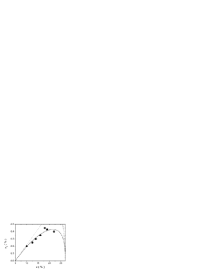
FIG. 28.: $y_{c}$ versus $x$ for La_2-xSr_xCu_1-yZn_yO₄. $\bullet$ : Taken from Momono et al. [16]. The solid curve interpolates between the critical behavior of a 2D-QSI transition with $\overline{\nu}=1$ (dotted line: $y_{c}\left(x\right)=0.03\left(x-5\right)$) and a 3D-QNS transition with $\overline{\nu}=1/2$ (dashed line: $y_{c}\left(x\right)=0.46\left(27-x\right)^{1/2}$).

The picture we no have is summarized in the phase diagram shown in Fig.3. The blue curve corresponds to the line of quantum phase transitions $y_{c}\left(x\right)$ shown in Fig.28. Along this line, $z\overline{\nu}=1$ is expected to hold (Eqs.(64) and (66)), while $\overline{\nu}\approx 1$(Eqs.(64)) at the 2D-QSI ($y=0$ and $x=x_{u}$) and $\overline{\nu}=1/2$ at the 3D-QSN (($y=0$ and $x=x_{o}$) transition. According to the empirical correlation between $T_{c}$ and anisotropy $\gamma_{T}$ (see Eq.(3) and Fig.2), the initial value of the dopant concentration determines whether the flow upon substitution leads to 2D-QSI or 3D-QSN criticality. For initially underdoped cuprates, the rise of $\gamma_{T}$ , tuned by the substitution induced reduction of $T_{c}$, drives the flow to 2D-QSI criticality. Conversely, in initially overdoped cuprates, the fall of $\gamma_{T}$  to a finite value directs the flow to 3D-QSN criticality. The mechanism whereby the substitution of Cu leads to a reduction of $T_{c}$ and finally to the quantum critical line $y_{c}\left(x\right)$ appears to be not well understood. When the aforementioned universality classes of the 2D-QSI and 3D-QSN transitions hold true (Eqs.(64) and (66)), disorder plays an essential role. At 2D-QSI criticality it localizes the pairs and destroys superfluidity[59, 60] and at the 3D-QSN transition it destroys superfluidity and the pairs[61]. In this context we also note that the phase diagram of La_2-xSr_xCuO_4+δ shown in Fig.4, reveals that isotope substitution leads to identical behavior, although less pronounced [27]. Since isotope substitution is accompanied by local lattice distortions, we conclude that in addition to disorder, lattice degrees of freedom tune superconductivity in an essential manner. Another essential facet emerges from the fact that the doping and substitution tuned flow to the 2D-QSI critical point is associated with an enhancement of $\gamma_{T}$. Thus, despite the fact that the fraction $\eta=\left(1/\lambda_{c}^{2}\left(0\right)\right)/\left(1/\lambda_{a}^{2}\left(0\right)+1/\lambda_{b}^{2}\left(0\right)+1/\lambda_{c}^{2}\left(0\right)\right)=1/\left(1+2\gamma_{T=0}^{2}\right)$[14], which the third dimension contributes to the superfluid energy density in the ground state, is very small, this implies that a finite $T_{c}$ is inevitably associated with an anisotropic but 3D condensation mechanism, because $\gamma_{T}$ is finite whenever superconductivity occurs (see Fig.2). This points unambiguously to the conclusion that theories formulated for a single CuO₂ plane cannot be the whole story. It does not imply, however, a 3D pairing mechanism because in the presence of fluctuations pairing and superfluidity occur separately.

D Evidence for magnetic field tuned quantum phase transitions

We have seen (Sec.IIB) that a strong magnetic field destroys superconductivity at finite temperature. In sufficiently clean systems this destruction occurs at the first order vortex melting transition. However, in the presence of disorder, the long-range order of the vortex lattice is destroyed and the vortex solid becomes a glass[29]. The vortex fluid to glass transition appears to be a second-order transition, signaled by the vanishing of the zero-frequency resistance in the vortex glass phase. Since disorder plays an essential role at 2D-QSI and 3D-QSN criticality, one expects a line $H_{m}\left(x\right)$ of vortex-glass to fluid quantum phase transitions, leading to the schematic phase diagram depicted in Fig.5.There is the superconducting phase (S), bounded by the zero-field transition line, $T_{c}\left(x,H=0\right)$, the critical lines of  the vortex melting or vortex glass  to vortex fluid transitions, $T_{m}\left(x=fixed,H\right)$ and the line of quantum critical points, $H_{m}\left(x,T=0\right)$. Along this line superconductivity is suppressed and the critical endpoints coincide with the 2D-QSI and 3D-QSN critical points at $x_{u}$ and $x_{o}$, respectively. To fix the critical line $H_{m}\left(x,T=0\right)$ close to the 2D-QSI and 3D-QSN transitions, we note that the singular part of the ground state energy density scales in analogy to Eq.(36) as

$$f_{s}\left(\delta,T\right)=\overline{Q}_{D}\left(\overline{\xi}_{\tau,0}^{-}\prod\limits_{i=1}^{D}\overline{\xi}_{i,0}^{-}\right)^{-1}\delta^{\overline{\nu}\left(D+z\right)}\overline{G}_{D}\left(\overline{z}\right),\ \ \ \overline{z}={{\frac{H\overline{\xi}_{a}\overline{\xi}_{b}}{\Phi_{0}}}}$$ (81)

where $H$ corresponds to a field applied parallel to the $c$-axis. Supposing that in the ($H,\delta$)-plane there is a continuous transition first order melting transition. Then the scaling function $\overline{G}_{D}\left(\overline{z}\right)$ will exhibit a singularity at some universal value $\overline{z}=\overline{z}_{m}$ . Thus close the 2D-QSI and 3D-QSN critical endpoints the quantum critical line (see Fig.5) is given by,

$$H_{m}\left(\delta\right)=\frac{\overline{z}_{m}\Phi_{0}}{\xi_{a,0}\xi_{b,0}}\ \delta^{2\overline{\nu}},$$ (82)

with $\overline{\nu}\approx 1$ (Eq.(64)) and $\overline{\nu}\approx 1/2$ (Eq.(66)) close to 2D-QSI and 3D-QSN criticality, respectively. Moreover, the singular behavior of the scaling function $\overline{G}_{D}\left(\overline{z}\right)$ must be such as enable the correlation length when $H\neq 0$ to correspond to the vortex glass transition, so that

$$\overline{\xi}_{H}=\overline{\xi}_{H,0}\left|\frac{H-H_{m}\left(\delta\right)}{H_{m}\left(\delta\right)}\right|^{-\overline{\nu}_{m}}.$$ (83)

$\overline{\nu}_{m}$ is the correlation length exponent of the vortex glass to fluid transition. Noting that $T_{c}\propto\delta^{\overline{\nu}z}\propto\xi^{-z}$ (see Eqs.(34) and (38), we obtain with Eq.(83) for the magnetic field induced reduction of $T_{c}$ the relation

$$T_{c}\left(H\right)\propto\left(H_{m}\left(\delta\right)-H\right)^{\overline{\nu}_{m}z_{m}}.$$ (84)

$z_{m}$ is the dynamic critical exponent of the vortex glass to fluid transition.

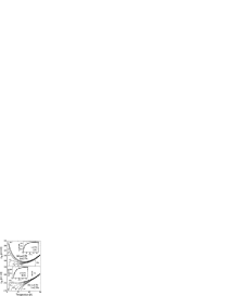
FIG. 29.: Left panel: In-plane resistivity $\rho_{ab}$ versus $T$ at $H=0,\ 4,\ 8,\ 16$ and $18T$ for YBa₂Cu_3-zZn_zO_y. a: $y=6.7,z=2.7\%$ and b: $y=6.7,z=2.3\%$. Taken from Segawa et al. [32]. Right panel: Schematic ($H,T$)-phase diagram of YBa₂Cu_3-zZn_zO_y derived from the data shown in the left panel.

The existence of a quantum phase transition line $H_{m}\left(\delta\right)$ can be anticipated from the in-plane resistivity data for YBa₂Cu_3-zZn_zO_y of Segawa et al. [32] shown in the left panel of Fig.29. With increasing magnetic field strength $T_{c}$ is depressed. In the sample with $y=6.7$ and $z=2.7\%$ the temperature dependence of $\rho_{ab}$ clearly points to a magnetic field tuned QSI transition around $16<H_{m}\left(y=6.7,z=2.7\%\right)\lesssim 18T$. Since $H_{m}\left(\delta\right)$ scales as $\ \delta^{2\overline{\nu}}\propto\left(z_{c}-z\right)^{2\overline{\nu}}$(Eq.(82)), $H_{m}\left(y=6.7,z\right)$ should increase with reduced Zn concentration $z$. This behavior is consistent with the data for $z=2.3\%$, where $H_{m}\left(y=6.7,z=2.3\%\right)>18T$. The emerging ($H,T$) phase diagram, consisting of finite temperature transition lines (vortex glass to fluid transitions) with 2D-QSI critical endpoints is displayed in the right panel of Fig.29. In the schematic ($x,H,T$)-phase diagram shown in Fig.5, these lines result from cuts near the zero field 2D-QSI-transition with $x$ replaced by $z$.

FIG. 30.: Left panel: Phase diagram of Bi₂Sr_2-xLa_xCuO_6+δ in the doping concentration (x or p)-temperature plane. Taken from Ono et al. [33]. Right panel: Temperature dependence of $\rho_{ab}$ for a Bi₂Sr_2-xLa_xCuO_6+δ crystal in H = 0 and 60 T for various dopant concentrations x. The insets shows a clearer view of the low temperature behavior for x=0.66 and 0.73. Taken from Ono et al.[33].

Related behavior was also observed in La_2-xSr_xCuO₄ [31] and Bi₂Sr_2-xLa_xCuO_6+δ [33]. In the hole doped La_2-xSr_xCuO₄ [31] and the electron doped $\Pr_{2-x}$Ce_xCu_4+δ a magnetic field tuned metal to insulator crossover was observed close to optimum doping, while in Bi₂Sr_2-xLa_xCuO_6+δ [33] the crossover sets in well inside the underdoped regime. The phase diagram of Bi₂Sr_2-xLa_xCuO_6+δ is displayed in the left panel of Fig.30. In the underdoped limit ($x\approx 0.84$ ) the transition temperature vanishes and a 2D-QSI transition is expected to occur. Evidence for this transition emerges from the temperature dependence of $\rho_{ab}$ shown in the right panel of Fig.30[33], taken at $H=0$ and $60T$ for six doping levels $x$. To strengthen this point we plotted in Fig. 31 the resulting $T_{c}$ versus $\rho_{0,c}-\rho_{0}$ for $x=0.76,0.73$ and $0.66$ and $\rho_{0,c}\approx 0.5$ $m\Omega cm$ at $H=0$. Apparently there is suggestive consistency with the 2D-QSI scaling relation (42) with $z\overline{\nu}\approx 1$, as well as with the corresponding data for La_2-xSr_xCuO${}_{4}\$ and YBa₂Cu₃O_7-δ shown in Fig.16. As the $60T$ data (symbols) are concerned, the samples closest to the QSI transition ($x=0.76$ and $0.84$)  exhibit in $\rho_{ab}$ a pronounced upturn at low temperatures. This points to an insulating normal state. Indeed, the weak upturn below $6$ $K$ at $x=0.73$, visible in the inset to Fig.30, signals the proximity to the onset of insulating behavior, while the low $T$ behavior of the $x=0.66$ sample with $T_{c}\left(H=0\right)$ $=23K$ exhibits metallic behavior. Thus, there is a metal to insulator (MI) crossover. The emerging ($x,T,H$)-phase diagram is displayed in Fig.32. The arrows mark the flows emerging from the experimental data displayed in Fig. 30 for $x=0.84$ (1) and $x=0.66$ (2).

FIG. 31.: $T_{c}$ versus $\rho_{0,c}-\rho_{0}$ for Bi₂Sr_2-xLa_xCuO_6+δ. Deduced from the data shown in Fig.30 for x=0.76, 0.73 and 0.66 and $\rho_{0,c}=0.5$ $m\Omega cm$. The straight line is the scaling relation (69) with $z\overline{\nu}\approx 1$.

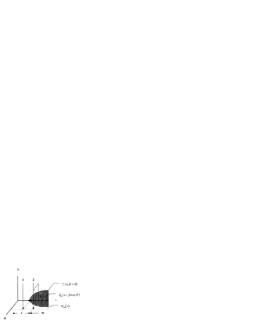
FIG. 32.: Schematic (x,T,H)-phase diagram close to the 2D-QSI transition. There is the superconducting phase (S), bounded by the zero-field transition line, $T_{c}\left(x,H=0\right)$, the lines of the vortex melting or vortex glass to vortex fluid transitions $T_{m}\left(x=fixed,H\right)$ and the quantum critical line $H_{m}\left(x\right)$. The critical lines $T_{c}\left(x,H=0\right)$ and $H_{m}\left(x\right)$ merge in the underdoped limit ($x=x_{u}$) where a doping driven quantum superconductor to insulator (QSI) transition ( $\bullet$ ) occurs. The arrows mark the flows emerging from the experimental data shown in Fig.31 at $x=0.84$ (1), $x=0.66$ (2).

This differs from the behavior observed in La_2-xSr_xCuO₄ where the detectable MI- crossover appears to set in close to optimum doping. In Fig.33 we depicted the logarithmic plot of $\rho_{ab}\left(T\right)$ for Bi₂Sr_2-xLa_xCuO_6+δ and La_2-xSr_xCuO₄ crystals for $H=0$ and $60T$ and various doping concentrations [33]. Concentrating on the presence or absence of an upturn, it is clearly seen that in La_2-xSr_xCuO₄ the MI-crossover occurs around $x\approx 0.15$, corresponding to optimum doping. However, it should be kept in mind that this crossover is nonuniversal. For this reason, the dopant concentration where insulating behavior is detectable is expected to be material dependent.

The magneto resistance $\rho_{ab}\left(H,T\right)$ of underdoped La_2-x Sr_xCuO₄ films with $x\approx 0.048$ $\left(T_{c}=0.45K\right)$ and $0.051$ $\left(T_{c}=4K\right)$ was also studied in magnetic fields up to $0.5T$ and at temperatures down to $30mK$  [118]. The temperature dependence of $\rho_{ab}\left(H,T\right)$ of the film closest to the 2D-QSI transition $\left(x\approx 0.048,\ T_{c}=0.45K\right)$ was found to be consistent with $\rho_{ab}\propto exp\left(\left(T/T_{0}\right)^{1/3}\right)$ below $1K$ and for fields from $4$ to $6T$. Thus this study points to 2D-localization. On the other hand, the data of Ando et al.[30] (Fig.33) appears to be consistent with a logarithmic divergence of the normal-state resistivity down to $0.7K$ for $x=0.08$ and $H=$ $60T$, suggesting 2D weak localization. In any case, the evidence for 2D localization confirms an essential property of 2D-QSI criticality: disorder localizes the pairs and destroys superfluidity[59, 60].

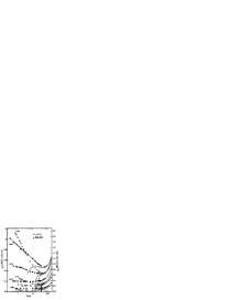
FIG. 33.: Logarithmic plot of $\rho_{ab}\left(T\right)$ for Bi₂Sr_2-xLa_xCuO_6+δ and La_2-xSr_xCuO₄ crystals in H=0T (solid lines) and 60 T (filled circles), labelled by La concentration, $x$. The straight line indicates consistency with the $log(1/T)$ behavior at $x=0.84$. and open circles are $H=30T$ data. La_2-x Sr_xCuO₄ data in $H=0T$ (dashed lines) and in $60T$ (open squares), labelled by the Sr concentration x. Taken from Ono et al.[33].

IV Thin films and field-effect doping

There is considerable evidence that the quantum superconductor to insulator transition in thin films can also be traversed by changing a parameter such as film thickness, disorder etc. [14]. As cuprates are concerned, an instructive example are the measurements of YBa₂Cu₃O_7-δ slabs of thickness $d$ separated by 16 unit cells ($\approx 187\ A$) of PrBa₂Cu₃O₇. Due to the large separation the YBa₂Cu₃O_7-δ slabs can be considered to be essentially to be uncoupled. As shown in Fig.6 in YBa₂Cu₃O_7-δ slabs of thickness $d$ the transition temperature was found to vary according to Eq.(4). Together with the scaling relation (38) this points to a 2D-QSI transition with $z\overline{\nu}=1$, in agreement with our previous estimate (Eq.(64)). Since quantum fluctuations alone are not incompatible with superconductivity, this 2D-QSI transition must be attributed to the combined effect of disorder and quantum fluctuations. For this reason it is conceivable that in cleaner films superconductivity may also occur at and below this value of $d_{s}$, which is close to the estimate derived from the bulk (Eq.(68)). Recently this has been achieved by inducing charges by the field-effect technique, whereby the mobile carrier density can be varied continuously and reversibly, without introducing additional sources of disorder[35, 36, 37]. By establishing a voltage difference between a metallic electrode and the crystal, charge can be added or removed from the CuO₂ layers: positive voltage injects electrons, and a negative voltage injects holes. This allows to vary both electron and hole charge densities over a considerable range of interest. Using this technique Schön et al.[37] converted an insulating thin slab of  CaCuO₂ into a superconductor. The success of this technique relies on the high quality films and on the quality of the interfaces between the film material and the metallic electrode. The ($T_{c}$, $x$) phase diagram for CaCuO₂ is shown Fig.7. The doping level was calculated from the independently measured capacitance of the gate dielectric, assuming that all the charge is located in a single CuO₂ layer. The diagram exhibits apparent electron and hole superconductivity, and bears a strong resemblance to results observed in other cuprates, in agreement with the empirical correlation (3). Note that the finite temperature superconductor to normal state transition falls into the 2D-XY universality class. Thus $T_{c}$ is the Kosterlitz-Thouless transition temperature. At low doping levels ($x<0.1$) a logarithmic divergence of $\rho$ was found. This observation for n- as well as p-type doping of CaCuO₂ are in accordance with a 2D-QSI transition in the underdoped limit, where disorder localizes the pairs and destroys superfluidity (Eq.(64)). Although superconductivity has been observed previously in SrCuO₂/BaCuO₂[38] and in BaCuO₂/CaCuO₂[39] superlattices with a maximum $T_{c}$ value of about 80 K, the field effect doping is not limited by dopant solubility and compositional stability. This technique allows to study the properties of a given material as a function of the dopant concentration without introducing additional disorder and additional defects. Because the charge carriers appear to be confined in a very thin layer, what’s seen is superconductivity in 2D. Thus, due to the reduced dimensionality fluctuations will be enhanced over the full range of dopant concentrations. The phase diagram displayed in Fig.7 also points to a 2D-QSN transition in the overdoped limit. A potential candidate is again the disordered metal to d-wave superconductor transition at weak coupling, considered by Herbut[61], with $z=2$ and $\overline{\nu}\approx 1/2$, and the system is in 2D right at its upper critical dimension. Clearly, more detailed studies are needed to uncover the characteristic 2D critical properties in field effect doped cuprates. Of particular relevance is the confirmation of the universal linear relationship between $T_{KT}$ and the zero temperature in-plane penetration depth $\lambda_{ab}\left(0\right)$ close to the 2D-QSI transition. This relation provides an upper bound for the attainable transition temperatures.

We saw that in the bulk (see e.g. Fig.2) and chemically doped films superconductivity disappears in the 2D-limit, while in field effect doped CaCuO₂ it survives. Since chemically doped materials with different carrier densities also have varying amounts of disorder, the third dimension is apparently needed to delocalize the carriers and to mediate superfluidity.

V Concluding remarks and comparison with other layered superconductors

Evidence for power laws and scaling should properly consist of data that cover several decades in the parameters. The various power laws which we have exhibited span at best one decade and the evidence for data collapse exists only over a small range of the variables. Consequently, though the overall picture of the different types of data is highly suggestive, it cannot really be said that it does more than indicate consistency with the scaling expected near a quantum critical point or a quantum critical line. Nevertheless, the doping, substitution and magnetic field induced suppression of $T_{c}$ clearly reveal the existence and the flow to 2D-QSI and 3D-QSN quantum phase transition points and lines (see Figs.1, 2, 3 and 5). In principle, their universal critical properties represent essential constraints for the microscopic theory and phenomenological models. As it stands, the experimental data is fully consistent with a single complex scalar order parameter, a doping induced dimensional crossover, a doping, substitution or magnetic field driven suppression of superconductivity, due to the loss of phase coherence. When the evidence for this scenario persists, antiferromagnetic and charge fluctuations are irrelevant close to criticality. Moreover, given the evidence for the flow to 2D-QSI criticality, the associated 3D-2D crossover, tuned by increasing anisotropy, implies that a finite $T_{c}$ and superfluid density in the ground state of bulk cuprates is unalterably linked to a finite anisotropy. This raises serious doubts that 2D models are potential candidates to explain superconductivity in bulk cuprates.Nevertheless, we saw that in sufficiently clean and field effect doped CaCuO₂ superconductivity survives in the 2D-limit. Thus, there is convincing evidence that the combined effect of disorder and quantum fluctuations plays an essential role and even destroys superconductivity in the 2D limit of chemically doped cuprates. Thus, as the nature of the quantum phase transitions in chemically doped cuprates is concerned, disorder is an essential ingredient. We have seen that the 2D-QSI transition has a rather wide and experimentally accessible critical region. For this reason we observed considerable and consistent evidence that it falls into the same universality class as the onset of superfluidity in ⁴He films in disordered media, corrected for the long-rangeness of the Coulomb interaction. The resulting critical exponents, $z=1$ and $\overline{\nu}\approx 1$ are also consistent with the empirical relations (Eqs.(1), (2) and (3)) and the observed temperature and magnetic field dependence of the specific heat coefficient in the limit of zero temperature. These properties also point to a 3D-QSN transition with $z=2$ and $\overline{\nu}\approx 1/2$, describing a d-wave superconductor to disordered metal transition at weak coupling. Here the disorder destroys superconductivity, while at the 2D-QSI transition it localizes the pairs and with that destroys superfluidity. Due to the existence of the 2D-QSI and 3D-QSN critical points, the detection of finite temperature 3D-XY critical behavior will be hampered by the associated crossovers which reduce the temperature regime where thermal 3D-XY fluctuations dominate. In any case, our analysis clearly revealed that superconductivity in chemically doped cuprate superconductors is a genuine 3D phenomenon and that the interplay of disorder (anisotropy) and superconductivity destroys the latter in the 2D limit. As a consequence, the universality of the empirical correlations reflects the flow to 2D-QSI and 3D-QSN criticality, tuned by chemical doping, substitution and an applied magnetic field. A detailed account of the flow from 2D-QSI to 3D-QSN criticality is a challenge for microscopic theories attempting to solve the puzzle of superconductivity in these materials. Although the mechanism for superconductivity in cuprates is not yet clear, essential constraints emerge from the existence of the quantum critical endpoints and lines. However, much experimental work remains to be done to fix the universality class of the 2D-QSI and particularly of the 3D-QSN critical points unambiguously.

In conclusion we note that universal properties emerging from thermal and quantum fluctuations are not restricted to cuprate superconductors. Potential candidates are the highly anisotropic organic superconductors which are close to a metal-insulator boundary. A glance to Fig.34 shows that the correlation between $\lambda_{c}\left(0\right)$ and $\sigma_{c}^{DC}\left(T_{c}^{+}\right)$ is particularly rewarding. In various classes of layered superconductors, including organics, transition metal dichalcogenides and cuprates, $\lambda_{c}\left(0\right)$ is systematically suppressed with increase of normal state conductivity $\sigma_{c}^{DC}\left(T_{c}^{+}\right)$. Without thermal and quantum fluctuations the DC conductivity is given by

$$\sigma_{c}^{DC}=\frac{ne^{2}}{m_{c}}\tau_{tr}=\frac{c^{2}\tau_{tr}}{4\pi\lambda_{c}^{2}\left(0\right)}.$$ (85)

$\tau_{tr}$ is the mean scattering time of the normal electrons in transport properties with number density per unit volume $n$ and effective mass $m_{c}$. Provided that the variations of $\tau_{tr}$ are small, superconductors where fluctuations can be neglected (mean-field superconductors) are then characterized by the dotted line in Fig.34, which is

$$\lambda_{c}\left(0\right)\propto\left(\sigma_{c}^{DC}\right)^{-1/2}.$$ (86)

It agrees with the data of mean-field superconductors rather well. Interestingly enough, MgB₂ and Sr₂RuO₄ appear to fall into this class, as well. Prominent and systematic deviations from this behavior occur for the highly anisotropic organics and underdoped cuprates. As $\lambda_{c}\left(0\right)$ increases with the reduction of the normal state conductivity $\sigma_{c}^{DC}$, we observe that the data tends to scatter around two branches, consistent with $\lambda_{c}\left(0\right)=\Omega_{s}\left(\sigma_{c}^{DC}\right)^{-3/4}$, which is the scaling relation (57) with $z=1$, describing the critical behavior close to 2D-QSI critical points. The most prominent deviations from these trends occur for overdoped cuprates (see also Fig.24). In particular the data for overdoped YBa₂Cu₃O${}_{7-\delta\text{ }}$(YBCO) exhibit an upturn, signaling the crossover to 3D-QSN criticality (Eq.(62)). Since organics undergo superconductor to insulator transitions[161], are highly anisotropic and $\gamma$ can be varied over a rather extended interval, i.e. $\gamma_{T_{c}}=180$ for $\kappa$-(ET)₂ Cu[N(CS)₂ ]Br, $\gamma_{T_{c}}=350$ for $\kappa$-(ET)₂ Cu(NCS)₂[162] and. $\gamma_{T_{c}}=2\ 10^{3}$ for $\alpha$- (BEDT-TTF)₂NH₄Hg(SCN)₄, it becomes clear that the organics line in Fig.34 indicates the flow of this class of superconductors to 2D-QSI criticality, where the scaling relation (57) applies.

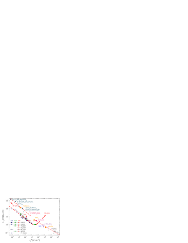
FIG. 34.: $\lambda_{c}\left(0\right)$ versus $\sigma_{c}^{DC}$ for a variety of superconductors partially collected by Dordevicet al.[119]. YBa₂Cu₃O_7-δ (YBCO)[120, 121, 122, 123, 124], La_2-xSr_xCuO_4+δ (LSCO)[122, 125, 126], HgBa₂CuO_4+δ (Hg1201)[127], Tl₂Ba₂CuO_6+δ (Tl2201)[128, 129, 130], Bi₂Sr₂CaCu₂O_8+δ (Bi2212)[131, 132], Nd_2-xCe_xCuO_4+δ(NCCO)[133]. Blue points -underdoped (UD), green -optimally doped (OpD) and red -overdoped (OD). Transition metal dichalcogenides[150, 151]; (ET)₂X compounds[141, 142, 143, 144, 145, 146, 147, 148, 149]; (TMTSF)₂ClO₄[134, 135, 136, 137, 138, 139, 140]; Sr₂RuO₄ [152, 153]; MgB₂[154, 155, 156]; Nb[157, 158]; Pb[158]; Nb Josephson junctions [159]; $\alpha$Mo_1-xGe_x[160]. The dotted line is Eq.(86) and the dashed ones Eq.(57). The red arrows indicate the flow to 2D-QSI and for overdoped YBa₂Cu₃O_7-δ to 3D-QSN criticality, respectively.

Thus unlike the organics the cuprates undergo a doping tuned crossover from 2D-QSI to 3D-QSN criticality, where $\sigma_{c}^{DC}\left(T_{c}^{+}\right)$ and $\lambda_{c}\left(0\right)$ tend to infinity, while $T_{c}$ vanishes. These critical points are attained in the underdoped and overdoped limit, respectively, where $T_{c}$ vanishes. In this crossover the cuprates either pass the organics or the dotted mean-field line, spanned by conventional superconductors (see Fig.34). YBa₂Cu₃O_7-δ(YBCO) and La_2-xSr_xCuO_4+δ(LSCO) cross the dotted mean-field line in the neighborhood of TaS₂, Sr₂RuO₄ and MgB${}_{2\text{ }}$. In this region of the $\lambda_{c}\left(0\right)$-$\sigma_{c}^{DC}\left(T_{c}^{+}\right)$ plane fluctuations do not play a dominant role. Indeed, Sr₂RuO₄ exhibits Fermi liquid normal state properties[163]. However, overdoped cuprates flow to 3D-QSN criticality, where disorder destroys the phase coherence and the pairs. On the contrary, the organics evolve rather smoothly from the mean-field regime, to which Pb, Nb, Nb-junctions, $\alpha$-Mo_1-xGe_x and the dichalcogenides belong. Thus, these flows provide a perspective of the regimes where fluctuations and disorder are essential.

It is a pleasure to thank H.Keller and K.A. Müller for numerous helpful discussions.

REFERENCES

-
[1]
Corresponding author: T.Schneider
Email address: toni.schneider@swissonline.ch - [2] M. Suzuki and M.Hikita, Phys. Rev. B 44, 249 (1991)
- [3] Y. Nakamura and S. Uchida, Phys. Rev. B 47, 8369 (1993))
- [4] Y. Fukuzumi et al., Phys. Rev. Lett. 76, 684 (1996)
- [5] M. Willemin et al., Phys. Rev. B 59, 717 (1999)
- [6] T.Kimura et al., Physica C 192, 247 (1992)
- [7] T. Sasagawa et al., Phys. Rev. B 61, 1610 (2000)
- [8] J. Hofer et al, Phys. Rev. B 62,631 (2000)
- [9] T. Shibauchi et al., Phys. Rev. Lett. 72, 2263 (1994)
- [10] C. Panagopulos et al., Phys. Rev. B 61, 3808 (2000)
- [11] J. L. Tallon et al., Phys. Rev. B 51, 12911 (1995)
- [12] M.R. Presland et al., Physica C 176, 95 (1991)
- [13] T. Schneider, Acta Physica Polonica A 91, 203 (1997)
- [14] T. Schneider and J. M. Singer, Phase Transition Approach To High Temperature Superconductivity, Imperial College Press, London, 2000
- [15] T.Schneider and J.M.Singer, J. of Superconductivity 13, 789 (2000)
- [16] N. Momono et al., Physica C 233, 395 (1994)
- [17] L. Onsager, Phys. Rev. 65, 117 (1944)
- [18] J. Hofer et al., Physica C 297, 103 (1998)
- [19] G. Xiao et al., Phys. Rev. B 42, 8752 (1990)
- [20] J.M. Tarascon et al., Phys. Rev. B 42, 218 (1990)
- [21] S. Watauchi et al., Phys. Rev. B 64, 64520 (2001)
- [22] T. R. Chien et al., Physica C 229, 273 (1994)
- [23] T.R. Chien et al., Phys. Rev. B 49, 1342 (1994)
- [24] T. R. Chien et al., Physica C 221, 428 (1994)
- [25] X. F. Sun et al., Phys. Rev. B 59, 8978 (1999)
- [26] C. Panagopoulos et al., Phys. Rev. B 54, 12721 (1996)
- [27] Guo-Meng Zhao et al., unpublished
- [28] G. Blatter et al., Rev. Mod. Phys. 66, 1125 (1994)
- [29] See, e.g., T. Schneider et al., Phys. Rev. B 63, 144527 (2001)
- [30] Y. Ando et al., Phys. Rev. Lett. 75, 4662 (1995)
- [31] G.S. Boebinger et al., Phys. Rev. Lett. 77, 5417 (1996)
- [32] K. Segawa et al., Phys. Rev. B 59, 3948 (1999)
- [33] S. Ono et al., Phys. Rev. Lett. 85, 638 (2000)
- [34] R. G. Goodrich, P. W. Adams, H. Lowndes and D. P. Norton, Phys. Rev. B 56, 14299 (1997)
- [35] C. H. Ahn et al., Science 269, 373 (1995)
- [36] T. Kawahara, N. Sugiuchi, E. Komai, T. Terashima and Y. Bando, Physica C 276,127 (1997)
- [37] J. H. Schön, M. Dorget, F. C. Beuran, X. Z. Zu, E. Arushanov, C. Deville Cavellin and M. Laguës, Nature 414, 434 (2001)
- [38] D. P. Norton et al., Science 265, 2074 (1994)
- [39] G. Balestrino et al., Phys. Rev. B 58, 8925 (1998)
- [40] T. Schneider and D. Ariosa, Z. Phys. B Cond. Mat. 89, 267 (1992)
- [41] T. Schneider and H. Keller, Int. J. Mod. Phys. B 8, 487 (1993)
- [42] M. A. Hubbard et al., Physica C 259, 309 (1996)
- [43] S. Kamal et al., Phys. Rev. Lett. 73, 1845 (1994); Phys. Rev. B 58, 8933 (1998)
- [44] V. Pasler et al., Phys. Rev. Lett. 81, 1094 (1998)
- [45] T. Schneider et al., Eur. Phys. J. B 3, 413 (1998)
- [46] T. Schneider and J. M. Singer, Physica C 341-348, 87 (2000)
- [47] K.Kim and P.B.Weichman, Phys. Rev. B 43, 13583 (1991)
- [48] S. Sachdev and J. Ye, Phys. Rev. Lett. 69, 2411 (1992)
- [49] P. Monthoux and D. Pines, Phys. Rev. B 50, 16015 (1994)
- [50] C. Castellani, C. Di Castro and M. Grilli, Phys. Rev. Lett. 75, 4650 (1995)
- [51] C. M. Varma, Acta Physica Polonica A 91, 191 (1997)
- [52] S. C. Zhang, Science 275, 1089 (1997)
- [53] S. Kivelson, E. Fradkin and V.J. Emery, Nature 393, 550 (1998)
- [54] M. Randeria, in Proceedings of the tenth International School of Physics ”Enrico Fermi ” Varenna, edited by G.Iadonisi and J.R. Schrieffer (IOS Press Amsterdam, 1998)
- [55] S. Capara et al., Phys. Rev. B 59, 14980 (1999)
- [56] S. Chakravarty et al., cond-mat/0005443
- [57] M. Voijta, Y. Zhang and S. Sachdev, Phys. Rev. Lett. 85, 4940 (2000)
- [58] P.W. Anderson, Science 288, 480 (2000)
- [59] M.P.A. Fisher et al., Phys. Rev. Lett. 64, 587 (1990)
- [60] I.F. Herbut, Phys. Rev. B 61, 14723 (2000)
- [61] I. F. Herbut, Phys. Rev. Lett. 85, 1532 (2000)
- [62] L. I. Glazman and A. E. Koshelev, Phys. Rev. B 43, 2835 (1991)
- [63] P. C. Hohenberg et al., Phys. Rev. B 13, 2986 (1976)
- [64] D. S. Fisher, M. P. A. Fisher and D. A.Huse, Phys. Rev. B 43, 130 (1991)
- [65] M.E. Fisher, M.N. Barber and D. Jasnow, Phys. Rev. A 8, 1111 (1973)
- [66] I. F. Herbut and Z. Tesanovic, Phys. Rev. Lett. 76, 4588 (1996)
- [67] W. F. Vinen, in Superconductivity II, edited by R. D. Parks (Marcel Dekker, INC., New York, 1969)
- [68] M. Charalambous et al., Phys. Rev. Lett. 83, 2042 (1999)
- [69] E. Schultka and E. Manusakis, Phys. Rev. Lett. 75, 2710 (1995)
- [70] E. S. Bozin, G. H. Kwei, H. Takagi and S. J. L. Billinge, cond-mat/9907017
- [71] K. M. Lang et al., cond-mat/0112232
- [72] A.W. Hunt, P.M. Singer, A.F. Cederstrom, and T. Imai, cond-mat/0011380)
- [73] A. Singsaas and G. Ahlers, Phys. Rev. B 30, 5103 (1994)
- [74] S. Mehta et al., J. Low Temp. Phys. 114, 467 (1999)
- [75] see, e.g. M. Ma, Modern Theory of Critical Phenomena, (Benjamin, Reading, 1976)
- [76] A. Junod, M. Roulin, B. Revaz and A. Erb, Physica B 280, 214 (2000)
- [77] S. L. Lee et al., Phys. Rev. Lett. 71, 3862 (1993)
- [78] A. Schilling et al., Phys. Rev. Lett. 78, 4833 (1997)
- [79] R. Liang et al., Phys. Rev. Lett. 76, 835 (1996)
- [80] M. Roulin et al., Physica C 296, 137 (1998)
- [81] M. Willemin et al., Phys. Rev. Lett. 81, 4236 (1998)
- [82] A. Schilling et al., Phys. Rev. B 58, 11157 (1998)
- [83] X. Hu et al., Phys. Rev. Lett. 79, 3498 (1997)
- [84] A. K. Nguyen and A. Sudbo, Phys. Rev. B 58, 2802 (1998)
- [85] M. Tinkham, Introduction to Superconductivity (Mc Graw Hill, New York, 1975)
- [86] L. N. Bulaevskii, Sov. Phys. JETP 37, 1133 (1973)
- [87] V. Ambegaokar and A. Baratoff, Phys. Rev. Lett. 10, 486 (1963)
- [88] G. Deutscher and O. Entin-Wohlman, J. Phys. C 10, L433 (1977)
- [89] P. A. Crowell, F. W van Keuls and J. R. Reppy, Phys. Rev. B 55, 12620 (1997)
- [90] Y.J. Uemura et al., Phys. Rev. B 38, 909 (1988), Y.J. Uemura et al., Rev. Lett. 62, 2317 (1989)
- [91] J. Perret, Thesis, University of Neuchatel (1999)
- [92] P. Zimmermann et al., Phys.Rev. B 52, 541 (1995)
- [93] C.L. Seaman et al., Phys.Rev. B 42, 6801 (1990)
- [94] T. Schneider and J. M. Singer, Physica C 313, 188 (1999)
- [95] K. Semba and A. Matsuda, Phys. Rev. Lett. 86, 496 (2000)
- [96] G.M. Zhao et al., J. Phys. Condens. Matter 10, 9055 (1998)
- [97] J. Hofer et al., Phys. Rev. Lett. 84, 4192 (2000)
- [98] R. Khasanov et al., cond-mat/0201165
- [99] P. Franck et al., Physica C 162-164, 733 ((1989), ibid. 185-189 (1991), Phys. Rev. B 44, 5318 (1991)
- [100] N. Babushkina et al., Physica C 185-189, 901 (1991)
- [101] H.J. Bornemann and D.E. Morris, Phys. Rev. B 44, 5322 (1991)
- [102] T. Schneider and H. Keller, Phys. Rev. Lett. 86, 4899 (2001)
- [103] S. J. Chen et al., Phys. Rev. B 58, 14753 (1998)
- [104] G. E. Volovik, JETP Lett. 58, 469 (1993)
- [105] H. Won and K. Maki, Europhys. Lett. 73, 2744 (1995)
- [106] J.W. Loram et al., 10 Ann. HTS Workshop ( World Scientifique 1996) p.341
- [107] C. Panagopoulos et al., Phys. Rev. B 60, 14617 (1999)
- [108] T. Jacobs et al., Phys. Rev. Lett. 75, 4516 (1995)
- [109] A. Shengelaya et al., Phys. Rev. B 58, 3457 (1998)
- [110] C. Bernhard et al., Phys. Rev. Lett. 86, 1614 (2001)
- [111] C. Niedermayer et al., Phys. Rev. Lett. 71, 1764 (1993)
- [112] D.N. Basov et al., Phys. Rev. B 50, 3511 (1994)
- [113] S. Uchida and K. Tamasaku, Physica C 293,1 (1997)
- [114] H. Shibata and A. Matsuda, Phys. Rev. B 59, 11672 (1999)
- [115] A. A. Abrikosov and L.P. Gorkov, Zh. Eksp. Teor. Fiz. 39, 1781 (1969) [Sov.Phys.-JETP 12, 1243 (1961)]
- [116] J. L. Tallon et al., Phys. Rev. Lett., 79, 5294 (1997)
- [117] J. L. Tallon, Phys. Rev., B 58, 5956 (1998)
- [118] K. Karpinska et al., Phys. Rev. Lett. 77, 3033 (1996)
- [119] S.V. Dordevic et al., cond-mat/0112042
- [120] D.N. Basov et al., Phys. Rev. B 50, 3511 1994
- [121] C.C. Homes et al., Physica C 254, 1 1995
- [122] S. Uchida and K. Tamasaku, Physica C 293, 1 1997
- [123] J. Schutzmann et al., Phys. Rev. Lett. 73, 174 (1994)
- [124] C. Bernhard et al., Phys. Rev. B 59, 6631 (1999)
- [125] D. N. Basov et al., Phys. Rev. B 52, 13141 (1995)
- [126] S. Uchida et al., Phys. Rev. B 53, 14558 (1996)
- [127] J.R. Kirtley et al., Phys. Rev. Lett. 81, 2140 (1998)
- [128] D. N. Basov et al., Science 288, 468 (2000)
- [129] K. A. Moler et al., Science 279, 1193 (1998)
- [130] A. Katz et al., Phys. Rev. B 61,5930 (2000)
- [131] J. R. Cooper et al., Nature 343, 444 (1990)
- [132] T. Motohashi et al., Phys. Rev. B 61, 9269 (2000)
- [133] A. Pimenov et al., Phys. Rev. B 62, 9822 (2000)
- [134] P. Garoche et al., Sol. Stat. Comm. 19, 455 (1976)
- [135] L. P. Le et al., Physica C 185-189, 2715 (1991)
- [136] J. J. Finley, Sol. Stat. Comm. 36, 493 (1980)
- [137] P. de Trey et al., J. Low Temp. Phys. 11, 421 (1973)
- [138] K. Onabe et al., J. Phys .Soc. Jap. 45, 50 (1978)
- [139] R. J. Kennedy et al., Can. J. Phys. 62, 776 (1984)
- [140] A. H. Thompson et al. Phys. Rev. B 5, 2811 (1972)
- [141] X. Su et al., Phys. Rev. B 58, 2944 (1998)
- [142] A. Carrington et al., Phys. Rev. Lett. 83, 4172 (1999)
- [143] T. Shibauchi et al., Phys. Rev. B 55, 11979 (1997)
- [144] M. Dressel et al., Phys. Rev. B 50, 13603 (1994)
- [145] H. Taniguchi et al., Phys. Rev. B 53, 8879 (1996)
- [146] S. Wanka et al., Phys. Rev. B 53, 9301 (1996)
- [147] K. Kajita et al., Sol. Stat. Comm. 64, 1279 (1987)
- [148] X. Su et al., Phys. Rev. B 59, 4376 (1999)
- [149] R. Prozorov et al., Phys. Rev. B 63, 052506 (2001)
- [150] H. Schwenk el al., Sol. Stat. Comm. 45, 767 (1983)
- [151] K. Murata et al., J. Phys. Soc. Jpn. 50, 3529 (1981)
- [152] Y. Maeno Y. et al., Nature 372, 532 (1994)
- [153] K. Yoshida et al., Physica C 263, 519 (1996)
- [154] C. Panagopoulos et al., cond-mat/0103060
- [155] M. Angst et al., cond-mat/0112166
- [156] D. K. Finnemore et al., Phys. Rev. Lett. 86, 2420 (2001)
- [157] A. V. Pronin et al., Phys. Rev. B 57, 14416 (1998)
- [158] O. Klein et al., Phys. Rev. B 50, 6307 (1994)
- [159] E. Goldobin et al., Phys. Rev. B 58, 15078 (1998)
- [160] S.J. Turneaure et al., Phys. Rev. Lett. 84, 987 (2000)
- [161] Y. Nakazawa et al., Phys. Rev. B 61, 16295 (2000)
- [162] S. Kawamata et al., J. Low. Temp. Phys. 105, 1721 (1996)
- [163] C. Bergemann et al., Phys. Rev. Lett. 84, 2662 (2000), and references therein.