Fluctuation Study of the Specific Heat of Mg¹¹B₂

Abstract

The specific heat of polycrystalline Mg¹¹B₂ has been measured with high resolution ac calorimetry from 5 to 45 K at constant magnetic fields. The excess specific heat above T_c is discussed in terms of Gaussian fluctuations and suggests that Mg¹¹B₂ is a bulk superconductor with Ginzburg-Landau coherence length $\xi_{0}=26$ Å. The transition-width broadening in field is treated in terms of lowest-Landau-level (LLL) fluctuations. That analysis requires that $\xi_{0}=20$ Å. The underestimate of the coherence length in field, along with deviations from 3D LLL predictions, suggest that there is an influence from the anisotropy of B_c2 between the c-axis and the a-b plane.

Experimental observations of thermodynamic fluctuations in the specific heat have been limited in low-T_c superconductors because the long coherence lengths make the excess specific heat very small compared to the mean-field term Skocpol and Tinkham (1975). By contrast, the high transition temperatures and small coherence lengths of cuprate superconductors lead to significant fluctuation effects Inderhees et al. (1988). In the recently discovered superconductor Mg¹¹B₂ Nakamatsu et al. (2001), the coherence length and superconducting transition temperature lie between these extremes, suggesting that fluctuation effects will be observable and lead to further information on the superconducting coherence length. Indeed, the excess magnetoconductance of Mg¹¹B₂ was reported recently and discussed in terms of fluctuation effects Kang et al. (2002). Here we report the specific heat of Mg¹¹B₂ from 5 K to 45 K at several magnetic fields. Using high resolution ac calorimetry, we could study the superconducting transition region in detail. At zero-field, the excess specific heat is treated in terms of 3D Gaussian fluctuations and in field, the broadening and shift of the transition is analyzed in terms of lowest-Landau-level (LLL) fluctuations.

Polycrystalline Mg¹¹B₂ was prepared at $T=950$ C and $p=3$ GPa from a stoichiometric mixture of Mg and ¹¹B isotope using a high-pressure synthesis method. Since the sample was synthesized at high pressure, there has been no additional annealing. Details of the synthesis can be found elsewhere Jung et al. (2001)^,Jung et al. (2002).

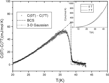
Figure 1: Temperature dependence of $\Delta C$ at zero field. The dash-dotted line is a BCS fit with $\Delta C_{\exp}$/$\gamma_{n}T_{c}=0.7$. The star represents a 3D Gaussian fluctuation model above T_c of 38.4 K. Inset: The temperature dependence of the specific heat at 0 and 7 T from 5 to 45 K.

Measurements of the heat capacity were based on an ac-calorimetric technique Kraftmakher (2001). A long cylindrical sample was cut into a disk by a diamond saw and then was sanded to a thin rectangular shape whose dimensions are approximately $1.1\times 1.5\times 0.1$ mm³; its mass is $375$ $\mu$g. The front face of the prepared sample was coated with colloidal graphite suspension (DAG) thinned with isopropyl alcohol to prevent a possible change of the optical absorption properties of the sample with temperature. The sample was weakly coupled to the heat bath through helium gas and suspending thermocouple wires. As a heating source, we used square-wave modulated laser pulse. The oscillating heat input incurred a steady temperature offset (or dc offset) from the heat bath with an oscillating temperature superposed. The ac part was kept less than 1/10 of the dc offset and was then converted to heat capacity by the relationship : $C\varpropto 1/T_{ac}$. The heat capacity obtained was converted to a specific heat by using a literature value above the superconducting temperature Bouquet et al. (2001a). The frequency of the periodic heating was chosen so that the $ac$ temperature was inversely proportional to the frequency and, therefore, to the heat capacity; $23$ Hz was used in this experiment. The $ac$ and $dc$ temperatures were measured by type E thermocouple, which were varnished on the back face of the sample using a minute amount of GE7031 diluted with a solvent of methanol and toluene. The GE varnish typically amounts to less than 1 % of the sample mass. Since the field induced error of type E thermocouple is less than 1 % at 40 K in 8 tesla, we will neglect the field dependence of the addenda contribution (DAG, GE-varnish, and type E thermocouple) and treat the field dependence as due only to the sample.

The inset in Fig.1 shows the temperature dependence of the specific heat at zero and 7 tesla from 5 to 45 K. The main graph is a plot of $\Delta C_{\exp}$ vs temperature at zero field. Here $\Delta C_{\exp}$ is the measured difference between the mixed- and normal-state specific heats. A 7-Tesla data set was used as a reference state above 20 K because it shows no observable transition in that range. The subtraction was executed without any smoothing of the 7-T data. The dash-dotted line is a BCS fit with the ratio of $\Delta C_{\exp}$/$\gamma_{n}T_{c}$ being variable Muhlschlegel (1959). The normal electronic coefficient $\gamma_{n}$ was set to be 2.6 mJ/mol K from the literature Bouquet et al. (2001a) and T_c of 38.4 K was determined from scaling discussed below. The best fit showed that the ratio is 0.7, which is much smaller than the weak coupling BCS value of 1.43. Since the ratio is generally larger for strong coupling superconductors, the small value does not tell us anything about its coupling strength. Recently, there has been a plethora of experimental and theoretical evidence which supports two-gap features in MgB2, which can explain the non-BCS jump magnitude with some success. Bouquet et al. (2001b); Wang et al. (2001); Yang et al. (2001); Liu et al. (2001); Choi et al. (2002) However, we cannot rule out such other scenarios as an anisotropic gap structure. Posazhennikova et al. (2002)^,Seneor et al. (2002) For a system in which fluctuation effects are pronounced, the experimentally determined transition temperature is lower than the mean-field critical temperature ($T_{c}^{mf}$) because fluctuations drive the system into the normal state even below $T_{c}^{mf}$. It is unlikely, however, that this can explain the large deviation from the BCS value.

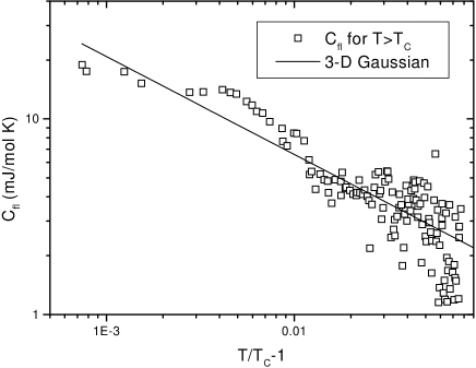
Figure 2: The excess specific heat, C${}_{fl}=\Delta C_{\exp}(0),$ for T ${>}$ T_c is plotted against reduced temperature $t=T/T_{c}-1$ on a log-log scale. The solid line describes Gaussian fluctuations for a bulk superconductor with a G-L coherence length of 26 Å.

Above the transition temperature, there is an excess specific heat tail apparent in Fig. 1. Thouless Thouless (1960) and subsequently Aslamazov and Larkin Aslamazov and Larkin (1968) showed that Gaussian fluctuations arise above T_c and predicted that $C_{fl}=C^{+}t^{-(2-d/2)}$ with $C^{+}=(k_{B}/8\pi)\xi_{GL}(0)^{-3}$, where $t=T/T_{c}-1,$ $d$ is the dimensionality, and $\xi_{GL}(0),$ the T=0 K Ginzburg-Landau coherence length. Figure 2 shows the temperature dependence of the excess specific heat on a log-log scale. The data follow a power law with an exponent of -0.5 and C${}^{+}=0.66$ mJ/mol K. The exponent indicates that Mg¹¹B₂ is a 3D superconductor and the substitution of C⁺ into the above formula gives $\xi_{GL}(0)=26\pm 1$ Å.

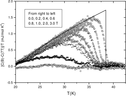
Figure 3: $\Delta C/T$ is plotted against temperature in B=0, 0.2, 0.4, 0.6, 0.8, 1.0, 2.0, and 3.0 tesla. Data were taken with increasing temperature after field cooling. The solid line represents a BCS fit.

When a magnetic field is applied, the specific heat broadens. Figure 3 shows the temperature dependence of $\Delta C/T$ at several magnetic fields. The ratio of the transition temperature shift to the transition width broadening in field is unique in that it is not as large as in low-T_c superconductors nor as small as in high-T_c materials. Its intermediate behavior is related to the fact that the coherence length and the superconducting transition temperature of Mg¹¹B₂ are intermediate between low-T_c and high-T_c superconductors. Lee and Shenoy Lee and Shenoy (1972) studied fluctuation phenomena in the presence of a magnetic field, arguing that bulk superconductors exhibit a field-induced effective change to one-dimensional behavior in the vicinity of the transition temperature $T_{c}(B)$. In a uniform magnetic field, the fluctuating Cooper pairs move in quantized Landau orbits and, close to upper critical field (B_c2), the lowest Landau level dominates the contribution to the excess specific heat. So, a bulk superconductor behaves like an array of one-dimensional rods parallel to the field. Thouless Thouless (1975) extended the idea above and below $T_{c}$ and suggested a scaling parameter for the fluctuation specific heat that is valid throughout the transition region :

$$\frac{\Delta C_{\exp}}{\Delta C_{mft}}=g\left(\frac{t}{\tau}\right),$$ (1)

where $t$ is the reduced temperature and $\tau$ is a field dependent dimensionless parameter that describes the superconducting transition width. The functional form $g(y)$ is model dependent. When a Hartree-like approximation Bray (1974) is used to examine the fluctuation effects of the quartic term in the free energy functional, it results in a simple form :

$$g(y)=\left(1+x(y)\right)^{-1},$$ (2)

$$y=x^{2/3}(1-2/x),$$ (3)

where $y=t/\tau(B)$.

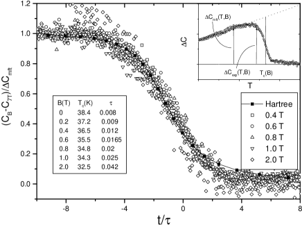
Figure 4: $\Delta C_{\exp}/\Delta C_{mft}$ vs $t/\tau$ is shown, where $\Delta C_{\exp}=C(B)-C(7T)$ and $\Delta C_{mft}$ are defined in the inset. Here $t$ is reduced temperature and $\tau$ is a field dependent dimensionless broadening parameter. Solid squares are from a Hartree-like approximation. Other field data were scaled so that they were collapsed onto the Hartree result. The obtained parameters (T_c, $\tau$) are tabulated inside the figure at each magnetic field. The inset sketches the definition of $\Delta C_{mft}(T,B)$ Farrant and Gough (1975)

In Fig. 4, the ratio of $\Delta C_{\exp}/\Delta C_{mft}$ in the transition region was plotted as $t/\tau(B)$, where $\Delta C_{\exp}(B)=C(B)-C(7T)$ and $\Delta C_{mft}$ was determined as in the classic work by Farrant and Gough Farrant and Gough (1975) by fitting the low temperature side of $\Delta C_{\exp}(B)$ as in Figs 1 and 3 and extrapolating linearly above T${}_{c}(B)$. A sketch is shown in the inset of Fig. 4. The scaling parameters $\tau(B)$ and T_c were chosen to make the data collapse onto the Hartree-like approximation (solid-squares). The values of $\tau(B)$ and T_c are listed in Fig. 4. The temperature dependence of the upper critical field T_c(B) is plotted in Fig. 5, and shows positive curvature close to $T_{c}(B=0)$. A simple empirical formula Sanchez et al. (1995), $B_{c2}(T)=B_{c2}(0)[1-(T/T_{c})^{2}][1-a(T/T_{c})^{2}]$, was used to describe the curvature, in which $a$ is a fitting parameter that is 0 and 0.3 for two-fluid model and for WHH model Werthamer et al. (1966) respectively. The best fit, solid line in Fig. 5, was produced with  $B_{c2}(0)=15.4$ $tesla$ and $a=0.8$. Positive curvature near $T_{c}(B=0)$ was also observed in non-magnetic rare-earth nickel borocarbides $RNi_{2}B_{2}C(R=Lu,Y)$ and could be explained by the dispersion of the Fermi velocity using an effective two-band model Shulga et al. (1998).

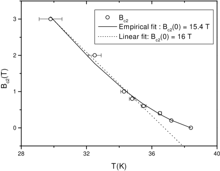
Figure 5: The temperature dependence of the upper critical field B${}_{c2}(T)$ is shown. The solid line is a simple empirical formula, $B_{c2}(0)[1-(T/T_{c})^{2}][1-a(T/T_{c})^{2}]$, with $a=0.8$ and $B_{c2}(0)=15.4$ T. The dotted line is a linear fit with $B_{c2}(0)=16$ T and $dB_{c2}/dT=-0.44$ $T/K.$

The broadening parameter $\tau$(B) consists of a field dependent part ($\tau_{B})$ and a field independent part ($\tau_{in})$. We postulate that they are independent of each other and add in quadrature, such that the total broadening is $\tau^{2}=\tau_{in}^{2}+\tau_{B}^{2}$. The field independent part was obtained in zero field and accounts for sample inhomogeneity and zero-field fluctuation effects while the field dependent part is due solely to field-induced fluctuations. The field dependence of the broadening parameter is given by Thouless (1975) :

$$\tau_{B}=\left(\frac{B}{B_{W}}\right)^{1/\alpha},$$ (4)

$$B_{W}=\left(\frac{\Delta C}{k_{B}/8\pi\xi_{0}^{3}}\right)B_{S},$$ (5)

where $\alpha=2-(d-2)/2$ ($\alpha=3/2$ for a bulk superconductor) and $B_{S}=-T_{c}(dB_{c2}/dT)_{T_{c}}$ in the mean-field scheme. The exponent $d-2$ indicates a dimensional crossover from d-dimension to d–2 behavior. The shift field $B_{S}$ is a characteristic field that sets the scale of the shift of the transition temperature while $B_{W}$ sets the scale of the width broadening of the transition region. In a standard superconductor, the ratio $B_{W}/B_{S}$ is very large ($\sim 10^{4}$), and the transition is shifted much more rapidly in field than it is broadened. In high temperature superconductors, such as YBCO, the broadening is as large as the shift ($B_{S}\sim B_{W})$, which is an indication that a mean-field approach based on a perturbation expansion might not be proper and that fluctuations should be treated in the context of critical phenomena. In Mg¹¹B₂, the ratio is in the order of 10², which is in between those two extremes. This feature seems consistent with other properties that show aspects of both conventional and high T_c superconductors. In order to study the anomalous broadening in field, we plot $\tau_{B}$ vs $(B/\Delta C)$ on a log-log scale in Fig. 6. The slope represents the exponent (1/$\alpha$) while the coefficient of the slope $\beta$ is related to the Ginzburg-Landau coherence length through $\beta=(k_{B}/8\pi\xi_{0}^{3}B_{S})^{1/\alpha}$. The lowest-Landau-level approximation is shown as a solid line having a slope of 2/3 and coefficient 2.7 $($A/m K$)^{2/3}$. From the coefficient of the fit, the Ginzburg-Landau coherence length is estimated to be 20 Å. In the above analysis, the shift field $B_{S}$ of 16 tesla was obtained by fitting the linear region of $B_{c2}$ (see Fig. 5).

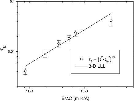
Figure 6: Field-broadened dimensionless parameter $\tau_{B}$ is plotted against $B/\Delta C$ on a log-log scale. The parameter was obtained by using $\tau_{B}=(\tau^{2}-\tau_{in}^{2})^{1/2}$ and $\Delta C$ is a mean-field discontinuity at T_c. The solid line represents a lowest-Landau-level (LLL) fluctuation: $\tau_{B}=\beta(B/\Delta C)^{1/\alpha}$ with $\alpha=3/2$ and $\beta=2.7$ $(A/m\cdot K)^{2/3}$.

Before making any further conclusions, we discuss some of the assumptions that we made in the analysis. In the zero-field analysis, sample inhomogeneity has been neglected. Boron 11 isotope Mg¹¹B₂ has a T_c of 39 K while the excess specific heat extends well above 40 K. We might expect inhomogeneity effects to complicate the fluctuation analysis below the transition temperature but above T_c, where our analysis is concerned, the effect will be negligible. However, when nonzero field is applied, sample inhomogeneity must be considered because the analysis is of the field dependent behavior of the transition region. Sample inhomogeneity could produce an additional broadening through the Ginzburg-Landau parameter $\kappa$ , and hence H_c2. Information on H_c2 slopes at different parts of the sample with different T_c’s would be needed to account for the additional broadening correctly. To be more precise, the H_c2 slope in the T_c = 39 K part of the sample and that in the, e.g., T_c = 38 K part would be needed. In our in-field analysis, we assumed that the slopes of H_c2 at different parts of the sample are same or if they are different, the difference is small, which leads to field independent inhomogeneity effect. It is necessary to study high quality single crystals with different T_c’s to better understand sample inhomogeneity effects on transition-width broadening.

In summary, the zero-field specific heat was discussed in the context of BCS theory plus 3D Gaussian fluctuations. The analysis indicates that Mg¹¹B₂ is a bulk superconductor and its coherence length is about 26 Å. In-field specific heat was treated in terms of lowest-Landau-level fluctuations. That analysis requires that $\xi_{0}=20$ Å. The in-field analysis could be complicated due to the effect of anisotropy in a polycrystalline sample. The anisotropy of $B_{c2}$ between ab-plane and c-axis directions can lead to a field dependent broadening due to the T_c distribution arising from the randomly oriented grains of the present sample. This in turn leads to an underestimation of the G-L coherence length. In order to understand the influence of anisotropy, we can assume that the transition broadening arises solely from $B_{c2}$ anisotropy and calculate the required anisotropy in our experimental temperature range. The reported anisotropy value of $\sim$3 from single crystal measurements Xu et al. (2001)^,Lee et al. (2001)^,Kim et al. (2002) is much smaller than the ratio 6 required to explain the broadening. From this consideration, we conclude that the anisotropy alone cannot explain the whole broadening and therefore that fluctuation effects should be considered in explaining the anomalous broadening.

This work at Urbana was supported by NSF DMR 99-72087. And the work at Pohang was supported by the Ministry of Science and Technology of Korea through the Creative Research Initiative Program.

References

- Skocpol and Tinkham (1975) W. J. Skocpol and M. Tinkham, Rep. Prog. Phys. 38, 1049 (1975).
- Inderhees et al. (1988) S. E. Inderhees, M. B. Salamon, N. Goldenfeld, J. P. Rice, B. G. Pazol, and D. M. Ginsberg, Phys. Rev. Lett. 60, 1178 (1988).
- Nakamatsu et al. (2001) J. Nakamatsu, N. Nakagawa, T. Muranaka, Y. Zenitani, and J. Akimitsu, Nature 410, 63 (2001).
- Kang et al. (2002) W. N. Kang, K. H. P. Kim, H.-J. Kim, E.-M. Choi, M.-S. Park, M.-S. Kim, Z. Du, C. U. Jung, K. H. Kim, S.-I. Lee, et al., J. Korean Phys. Soc. 40, 949 (2002).
- Jung et al. (2001) C. U. Jung, M.-S. Park, W. N. Kang, M.-S. Kim, K. Kim, and S.-I. Lee, Appl. Phys. Lett. 78, 4157 (2001).
- Jung et al. (2002) C. U. Jung, H.-J. Kim, M.-S. Park, M.-S. Kim, J. Y. Kim, Z. Du, S.-I. Lee, K. H. Kim, J. B. Betts, M. Jaime, et al., Physica C 366, 299 (2002).
- Kraftmakher (2001) Y. Kraftmakher, Phys. Rept. 356, 1 (2001).
- Bouquet et al. (2001a) F. Bouquet, R. A. Fisher, N. E. Phillips, D. G. Hinks, and J. D. Jorgensen, Phys. Rev. Lett. 87, 047001 (2001a).
- Muhlschlegel (1959) B. Muhlschlegel, Z. Phys. 156, 313 (1959).
- Bouquet et al. (2001b) F. Bouquet, Y. Wang, R. A. Fisher, D. G. Hinks, J. D. Jorgensen, A. Junod, and N. E. Phillips, Europhys. Lett. 56, 856 (2001b).
- Wang et al. (2001) Y. Wang, T. Plackowski, and A. Junod, Physica C 355, 179 (2001).
- Yang et al. (2001) H. D. Yang, J. Y. Lin, H. H. Li, F. H. Hsu, C. J. Liu, and C. Jin, Phys. Rev. Lett 87, 167003 (2001).
- Liu et al. (2001) A. Y. Liu, I. I. Mazin, and J. Kortus, Phys. Rev. Lett. 87, 87005 (2001).
- Choi et al. (2002) H. J. Choi, D. Roundy, H. Sun, M. L. Cohen, and S. G. Louie, Phys. Rev. B 66, 020513 (2002).
- Posazhennikova et al. (2002) A. I. Posazhennikova, T. Dahm, and K. Maki, con-mat/0204272, sunbmitted to Europhys. Lett. (2002).
- Seneor et al. (2002) P. Seneor, C. T. Chen, N. C. Yeh, R. P. Vasquez, L. D. Bell, C. U. Jung, M.-S. Park, H.-J. Kim, W. N. Kang, and S.-I. Lee, Phys. Rev. B 65, 012505 (2002).
- Thouless (1960) D. J. Thouless, Ann. Phys. (N. Y) 10, 553 (1960).
- Aslamazov and Larkin (1968) L. G. Aslamazov and A. I. Larkin, Soviet Physics - Solid State 10, 875 (1968).
- Lee and Shenoy (1972) P. A. Lee and S. R. Shenoy, Phys. Rev. Lett. 28, 1025 (1972).
- Thouless (1975) D. J. Thouless, Phys. Rev. Lett. 34, 946 (1975).
- Bray (1974) A. J. Bray, Phys. Rev. B 9, 4752 (1974).
- Farrant and Gough (1975) S. P. Farrant and C. E. Gough, Phys. Rev. Lett. 34, 943 (1975).
- Sanchez et al. (1995) D. Sanchez, A. Junod, J. Muller, H. Berter, and F. Levy, Physica B 204, 167 (1995).
- Werthamer et al. (1966) N. R. Werthamer, E. Helfand, and P. C. Hohenberg, Phys. Rev. 147, 295 (1966).
- Shulga et al. (1998) S. V. Shulga, S. L. Drechsler, G. Fuchs, K. H. Muller, K. Winzer, M. Heinecke, and K. Krug, Phys. Rev. Lett. 80, 1730 (1998).
- Xu et al. (2001) M. Xu, H. Kitazawa, Y. Takano, J. Ye, K. Nishida, H. Abe, A. Matsushita, N. Tsujii, and G. Kido, Appl. Phys. Lett. 79, 2779 (2001).
- Lee et al. (2001) S. Lee, H. Mori, T. Masui, Y. Eltesev, A. Yamamoto, and S. Tajima, J. Phys. Soc. Jpn. 70, 2255 (2001).
- Kim et al. (2002) K. H. P. Kim, J.-H. Choi, C. U. Jung, P. Chowdhury, H.-S. Lee, M.-S. Park, H.-J. Kim, J. Y. Kim, Z. Du, E.-M. Choi, et al., Phys. Rev. B 65, 100510 (2002).