$SrCu_{2}(BO_{3})_{2}$: A Unique Mott Hubbard Insulator ${}^{\dagger\;*}$

Abstract

We discuss the recently discovered system $SrCu_{2}(BO_{3})_{2}$, a realization of an exactly solvable model proposed two decades earlier. We propose its interpretation as a Mott Hubbard insulator. The possible superconducting phase arising from doping is explored, and its nature as well as its importance for testing the RVB theory of superconductivity are discussed.

18 March 2002

Dedicated to Professor Bill Sutherland on occasion of his 60^th birthday.

1 Introduction

Quantum spin systems are of great current interest, as shown by this symposium, with roots in two distinct sources. On the one hand the theory of model systems providing a rich variety of possibilities, and on the other, the field of synthetic materials, which has generated a vast number of systems, often close to theoretical models. As a result of this interplay, several interesting systems have been made in the laboratory, challenging our understanding by producing not only the expected, but also on occasion, the unexpected. Such a system that has caught attention recently is $SrCu_{2}(BO_{3})_{2}$, a two dimensional $S=1/2$ isotropic Heisenberg antiferromagnet in two dimensions on a particular lattice with the property that it is solvable exactly for the ground state. Indeed it was solved two decades ago [1] by Sutherland and one of us. In this article we summarize the story so far, and also explore possible interesting physics that could arise if this system is doped.

The situation of exactly solvable models in the area of statistical mechanics is rather limited. There is a general feeling that the special models are non-generic and rare, and hence somewhat ornamental. Enlightened opinion[2] has been more positive, and indeed the role of some solvable models is very well recognized. In contrast, the situation in condensed matter physics is very positive. The interaction between new systems, new phenomena and novel concepts has been rewarding. The table below gives a few examples of popular systems, their realizations and the unique concepts associated with them.

Year	Model Systems	Realization	New Concepts
1930	one dimensional Heisenberg Bethe AFM	CPC, CuO chains	Quantum Disorder, Spinons
1968	one dimensional Majumdar Ghosh AFM	(approximate mapping) $CuGeO_{3}$	Broken Discrete Symmetries and Spinons
1969-87	one dimensional $1/r^{2}$ Calogero, Sutherland, Haldane, Shastry systems	Parametric Correlations in Quantum Chaos	Spinons, Unusual Statistics
1969	one dimensional Hubbard Model	Benzene, Annulenes	Spin Charge Separation, Holons, Spinons, SC Fluctuations from repulsion, Mott Hubbard Insulating state
1988	one dimensional Spin-1 Heisenberg AFM, Affleck, Kennedy, Lieb and Tasaki chain	Ni Chains, NENP	Haldane Spin Gap
1990	one dimensional n leg Heisenberg Ladders	Vanadates $CaV_{n}O_{2n+1}$	Integer vs non integer phenomena, Superconductivity from doping Insulators
1981	two dimensional S=1/2 Shastry Sutherland model	$SrCu_{2}(BO_{3})_{2}$	Dimer states, Magnetization Plateaus…

The $1/r^{2}$ system in this table is different from the rest in that the physical realization comes from the world of quantum chaos, the continuum model is the description of parametric correlations in chaotic systems. The sole two dimensional system in the list is the main concern of this article. It has for long been unique in its very existence as a two dimensional member of the family of solvable models. It is particularly surprising since it is a model with essential simplicity as evidenced by the absence of crossed bonds. It is now even more remarkable in that nature finds a way of fulfilling the conditions for solvability in the compound $SrCu_{2}(BO_{3})_{2}$. We discuss the origin of the model, its discovery in real life, some recent interesting developments in the physical properties, and some possible future directions.

1.1 Origin of the model

In view of the enormous current interest in the problem, and also questions from colleagues, it may not be inappropriate to say a few words on the Shastry Sutherland (SS) model on a special lattice, and how it came about. In 1980, I (BSS) joined the University of Utah as a junior faculty member in the group consisting of Professors D C Mattis and B Sutherland. After an inspiring talk from Professor J R Schrieffer on polyacetylene, I mentioned to Professor Sutherland that a clear magnetic analog of polyacetylene ground state is the Majumdar Ghosh (MG) model, the one dimensional Heisenberg with a second neighbour interaction half as strong as the first. Professor Majumdar, my PhD advisor at TIFR in Bombay earlier, had invented this model in an effort to go beyond the Bethe nearest neighbour antiferromagnet ( AFM). The model was well known to me, in spite of rather wise discouragement by Majumdar from working on Exactly Solvable models, as a discipline unconnected with traditional topics in Solid State and Many Body Physics, in view of the almost zero probability of finding a new one! I remember being surprised that Sutherland, already then a sensei in the area of exactly solvable systems, had not come across this model! In that characteristically American way, there was no gap between learning of a new thing and getting excited and plunging into. I also caught the excitement that I had carried, but so far resisted (!). We first came up with the soliton excitations of the MG model, the so called spinons, as isolated unpaired spin 1/2 propagating objects in the midst of a sea of singlet dimerized spins. These were identical to the solitons of Schrieffer in spirit, but fractionalized the spin degrees of freedom rather than charge. Such excitations have since become a paradigm in the post High Tc language of strongly correlated systems, where the fixed singlets of MG give way to dancing singlets, the Resonating Valence Bond States envisioned by Anderson.

In an effort to go beyond one dimension to higher dimensions, we tried various things. It was clear that a decomposition into triangles was the key to the MG model, and there was no essential reason why this had to be only one dimensional. The general point made was clear[3], the search for Integrable systems in higher dimensions is not very rewarding, the conditions for integrability seem hard to satisfy in higher than one dimension, however, the search for exactly solvable models ( for the ground state) is more promising a priori. In a $d$-dimensional Hilbert space there is a huge number ( $\sim d^{2}/2$)of, in general, non commuting operators that simultaneously share a given eigenstate, for example the dimer covering, and the search boils down to states and operators that satisfy the somewhat subjective criterion of “naturalness”. As a result we pondered for several weeks on likely systems such as the two dimensional triangular lattice, where it became clear that no dimer like states work since the triangles share bonds with more than one other triangle. One needed a lattice where for a given triangle, no more than one bond is shared with another. This line of thinking led to the SS lattice shown in Fig.1(a).

Figure 1: The SS lattice. The angle $\theta$ is the apical angle for triangles that are the building blocks of the lattice, and by continuously changing it, one generates different looking lattices with essentially identical topology. (a) represents the original choice of SS, and (c) the case closest to the Copper lattice of $SrCu_{2}(BO_{3})_{2}$.

The proof of the ground state is simple and worth repeating if only briefly. The Hamiltonian can be written as a sum over triangles

$$H=J\Sigma_{t}H_{t}=J\left(\sum_{<i,j>}\vec{S}_{i}.\vec{S}_{j}+2\alpha_{SS}\sum_{<l,m>}\vec{S}_{l}.\vec{S}_{m}\right)$$ (1)

where the subscript $t$ refers to triangles, with $H_{t}=\alpha_{SS}\vec{S}_{1}.\vec{S}_{2}+(\vec{S}_{1}+\vec{S}_{2}).\vec{S}_{3}$,   $\alpha_{SS}$ is the bond strength parameter, sites $1,2$ refer to the two sites on the diagonal and $3$ the third site. Here and later we will denote the “dimer” bonds by $l,m$ and the non dimer nearest neighbours as $i,j$. The first, and remarkable point is that the dimer state $\psi=\prod_{l<m}[l,m]$ is an eigenstate of $H$. Here the product runs over all dimers on the lattice, which must provide a covering of the lattice ( i.e. every lattice point must occur once and only once in the product). This happens because we can rearrange the operation of the Hamiltonian into two classes of terms, the wanted and the unanted terms. The wanted terms isolate the spin interactions on the dimer spins. Remarkably all unwanted terms have the form $\vec{S}_{j}.(\vec{S}_{1}+\vec{S}_{2})[1,2]$, for appropriate indices, which vanishes on using the singlet property. By Rayleigh Ritz variational principle $E_{dimer}\geq E_{0}$, but by the Anderson decomposition strategy we have a lower bound $E_{0}\geq N_{t}e_{t}$. Happily the upper and lower bounds coincide for $\alpha_{SS}\geq 1$, and we are guaranteed that this is the ground state. Later work[15] improves this lower bound on $\alpha_{SS}$ somewhat to $\sim 0.74$.

These dimer ground states in two dimensions turn out to be surprisingly robust, for example the coupling constant $\alpha_{SS}$ is determined by an inequality rather than an equality, so there is an entire phase where the dimer states are the ground state, unlike the one dimensional case where one has a solution at isolated points only. This clearly greatly increases the probability of finding such models realized in nature, whereas in one dimension we should only expect proximities. Further the ground state is insensitive to the spin space isotropy of the underlying Hamiltonian, and one has the strange situation where the ground state has a greater symmetry than of the Hamiltonian! The phrase “superstability” [3] describes this kind of robustness shared by most of the dimer ground state systems. An example of robustness comes from later in the story, where we find that the ground state of stacks of the SS lattice, rotated by $\pi/2$ and coupled by vertical spin interactions, a model that describes the real 3-d material $SrCu_{2}(BO_{3})_{2}$, “magically” manages to have the dimer state as the true ground state[4]!

1.2 The system $SrCu_{2}(BO_{3})_{2}$

Almost two decades later, Kageyama and coworkers at the ISSP in Tokyo found that $SrCu_{2}(BO_{3})_{2}$, synthesized earlier in 1991 by Smith and Keszler, had very unusual properties. The spin $1/2$ moments of Copper living in well isolated two dimensional layers seemed to lock up into singlets, and a clear spin gap behaviour was observed by NMR. They concluded that this is a unique system, the first truly two dimensional spin gapped system with $S=1/2$. The data was analyzed by Mihayara and Ueda (MU)[4], who realized that the physical system was describable by an exactly solvable model. They proposed the model, found its solution, and then realized that it was essentially (topologically) the same model as SS, but looked different due to the details of the lattice. The Copper lattice is shown in Fig.1(c), and by opening up the angle $\theta$ continuously, one reaches the SS lattice ( with $\theta=\pi/2$ ). An intermediate value of $\theta=\pi/4$ in Fig.1(b) aids the imagination. Changing the angle $\theta$ clearly preserves the orthogonality of the “dimer” bonds but changes the bond length relative to the inter dimer bond lengths. This is crucial, since the criterion for solvability $\alpha_{SS}\geq\sim 0.74$ becomes realizable only in this picture. A nice visualization of this deformation is available courtesy Dr H Kageyama at http://www.issp.u-tokyo.ac.jp/labs/mdcl/ueda/kage/head.html. The Hamiltonian is written by MU and some recent papers as $H=J[\alpha_{MU}\sum_{i<j}\vec{S}_{i}.\vec{S}_{j}+\sum_{l<m}\vec{S}_{l}.\vec{S}_{m}]$, with $J^{\prime}\equiv J\alpha_{MU}$, and hence we clearly have $\alpha_{SS}\cdot\alpha_{MU}=\frac{1}{2}$. The current estimates of ($J,\;\alpha_{MU}$) using experimental data on $SrCu_{2}(BO_{3})_{2}$ range from [4] ($85^{0}K,\;0.635$) to [5] ($71.5^{0}K,\;0.603$). Thus $\alpha_{SS}\sim 0.78$ is perilously close to, but on the safe side of the phase boundary at $\sim 0.74$.

1.3 Recent Developments

We next mention a few of the very large number of papers that have been written recently, with apologies in advance for possible incompleteness. After the discovery of the spin gap, neutron scattering has confirmed the absence of magnetic LRO and inelastic scattering has given clear indication of a flat dispersionless triplet excitation mode at about 3 meV, as well as of many branches of dispersing bound states of triplet excitations[6]. NMR experiments were the first to show the spin gap[7] at about 30 K. ESR experiments show the presence of a second gap at about 4.7 meV which implies a substantial binding energy of two triplets[8]. Raman studies show a singlet bound state at about 3.7 meV [9]. The magnetic exchange constants, as mentioned are in the 60-80 K range. This is convenient for exploring with available pulsed high magnetic field experiments, which reveal[7, 12] the surprising existence of magnetic plateaus at $M/M_{s}=1/4,1/3,1/8..$. There is interesting data on the effect of magnetic excitations on phononic thermal conductivity[10].

Thus a large set of experiments have already been done, and provide many constraints on the theory. We should mention that the knowledge of the exact solution of the ground state does not give much insight into the excitations in this class of systems. One knows that in general terms, the singlet dimers can be broken into triplets, and that isolated triplets find it hard to propagate on the SS lattice due to its topology. This leads to flat bands of triplet excitations, i.e. very massive objects, consistent with neutron data. Pairs of triplets, however, escape the topological constraints, much as holes in the Nèel Antiferromagnet, and move about quite freely. Thus one has kinetic binding and the bound state has substantial dispersion[11].

In a sense the unexpected and new physics so far has been the presence of these plateaus[12]. These are unique in that they are the first two dimensional plateaus seen, and have attracted considerable interest. Several possible scenarios have been suggested to explain these. One picture is that of massive triplet excitations acting as hardcore bosons, that hop as well as interact. The effective interactions are strong due to large mass, and Wigner crystallization is proposed to explain the plateaus[13]. Alternatively one can view this plateau formation as the Quantum Hall Effect of hard core bosons, and a Chern Simons type field theory provides a fair description. The structure of the Hofstadter spectrum on the SS lattice is reflected in the plateaus[14]. At the moment it is not easy to reach a conclusion as to the best interpretation, especially since the experiments do not show plateaus that have anything like the precision of the Quantum Hall Effect.

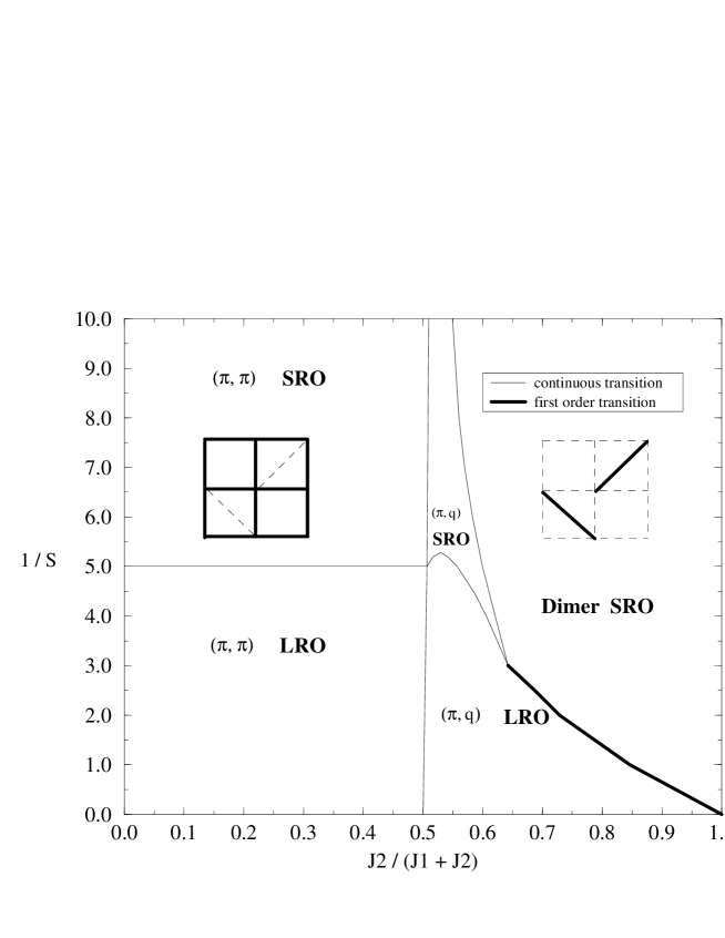
Figure 2: The phase diagram of Ref. [18] in the large N limit. The abscissa may be read as $2\alpha_{SS}/(1+2\alpha_{SS})$.

The phase diagram at zero field has come in for close scrutiny by several authors, using series expansion ideas[15, 16], rigorous bounds[17], large N field theories[18], as well as effective field theories of bosonic dimers[19]. Exotic and unusual intermediate phases are suggested by these studies, including[18] a “topologically ordered phase with deconfined $S=1/2$ spinons, which should give rise to an exotic superconductor with anomalous flux properties under doping”. An early paper by Albrecht and Mila[20] discusses the transition between the dimer and AFM phases using Schwinger Bosons, and concludes that it should be first order. A qualitatively new intermediate spin liquid phase with power law correlations has been proposed by Koga and Kawakami[15]. The phase diagram in Fig.2 is from reference [18] for a large $N$ theory, and represents a possible set of phases with various kinds of magnetic order. The Koga-Kawakami phase may be viewed as the SRO $(\pi,q)$ phase.

We should also mention new theoretical models that are generalizations of the SS ideas to higher dimensions and other systems[22, 21]. The beautiful model of Müller-Hartmann, Singh, Knetter and Uhrig [22] has a new set of exchange interactions added to the SS model, and had a very rich set of constants of motion. It is very tractable, giving rise to magnetization plateaus that are similar to but not identical to the experimental ones.

2 Mean Field Theory of the Doped Dimer Superconductor, a Possible test of RVB

In this section we discuss the possibility of doping the dimer state, and what one may expect from it. Firstly we remark that the insulating dimerized ground state of $SrCu_{2}(BO_{3})_{2}$ may usefully be considered as a Mott Insulating state of an underlying Hubbard model. To see this consider the Hubbard model on the SS lattice with

$$H=-t\sum_{<ij>,\sigma}(c^{\dagger}_{i\sigma}c_{j\sigma}+h.c.)-\alpha t\sum_{<l,m>,\sigma}(c^{\dagger}_{l,\sigma}c_{m,\sigma}+h.c.)+U\sum_{r}n_{r,\uparrow}n_{r,\downarrow}$$ (2)

where the (somewhat overused) symbol $\alpha$ represents the ratio of hoppings on the two kinds of bonds, and the Hubbard interaction term sums over all types of sites. Clearly the superexchange argument fixes it in terms of the ratio of the exchange parameters via $\alpha^{2}=2\alpha_{SS}$, and we note that $\alpha=\pm 1.25$ using the insulating state estimates, with the sign undetermined. In the non-interacting limit the band structure is interesting, we have four subbands, with the extrema of two of them touching quadratically at the zone center. At half filling, one has four electrons per unit cell and the system is a semi-metal with a finite density of states, and thus it has typical metallic behaviour such as a linear specific heat. A parallel may be drawn with the semi-metallicity of graphite on the hexagonal lattice with two electrons per unit cell and also of a fiduciary $MgB_{2}$ with well separated planes. In the case of graphite however, one has a “Dirac like” linear spectrum, and hence the density of states near the “fermi point” , i.e the contact point vanishes.

This semi-metal becomes an insulator at large enough $U$, undergoing a transition to the dimerized state that does not break rotation invariance nor the lattice translation symmetry, and may be called a Mott transition in the same sense as that of the one dimensional Hubbard model at half filling at infinitesimal $U$. Since the large $U$ behaviour is exactly known, namely the dimer ground state, further terms in the $t/U$ expansion beyond superexchange should be useful in elucidating the nature of the Mott transition here [23]. This transition has not yet been studied in literature. Starting from the semi-metal and turning on $U$, one may either have a level crossing transition to the gapped insulator, or more interestingly a continuous opening of the charge gap. In the gapped insulating phase, the four spin correlation function pertaining to dimer order $<S_{a}S_{b}S_{c}S_{d}>\sim<S_{a}S_{b}><S_{c}S_{d}>$, and thus there is ODLRO in this correlation function without any obvious symmetry that is broken. With this distinction, without necessarily a major difference, we may refer to $SrCu_{2}(BO_{3})_{2}$ as a Mott insulator.

Having this realization of the Mott Hubbard insulator, we naturally enquire if the philosophy of the RVB theory of Superconductivity due to Anderson applies here. This theory is built upon the idea that repulsive interactions of the Hubbard type lead to superconductivity via the intermediate step of superexchange, or Heisenberg interactions in the insulating state. The superexchange leads to singlet pairing between electrons of opposite spin, and these pairs are analogous to the Cooper pairs, but are localized due to the Mott-Hubbard gap. Under doping the Mott-Hubbard gap collapses, these preexisting pairs propagate freely, and lead to superconductivity. In the present case, the Cooper pairs at half filling should be viewed as the dimer-singlets, which on doping should move around by the same logic, and lead to superconductivity. Since the values of exchange are smaller by an order of magnitude from those in High Tc systems, we expect lower Tc’s, say tens of degrees K, but accompanied by the characteristic signature of singlet pairing and also of definite phase relations of Cooper pairs on the bonds, analogous to the d-wave pairing. While this theory is remarkably effective in providing a comprehensive view point, it still lacks unambiguous experimental support or a rigorous mathematical foundation, and one would welcome other supports to its validity or otherwise. In this context we work out in this section the mean field theory of a fiducial doped $SrCu_{2}(BO)_{3}$, and calculate some characteristics of the proposed superconducting compound.

Before doing so, let us note that doping can be of either chemical type, as in say $Sr_{1-x}M_{x}Cu_{2}(BO_{3})_{2}$ with a monovalent alkali $M$ or a trivalent lanthanide. However, one interesting possibility is suggested by the comparison of $MgB_{2}$ with graphite. One learns that $MgB_{2}$ is isoelectronic with graphite, but avoids being a semimetal by dispersing the bands in the direction transverse to the two dimensional sheets, it self-dopes by decreasing the transverse lattice constant. It is possible that a divalent element like $Mg$ in place of $Sr$ with a smaller ionic radius could decrease the transverse lattice constant of $SrCu_{2}(BO_{3})_{2}$ sufficiently so that it would have substantial transverse dispersion. We should clarify that unlike $MgB_{2}$ which appears to be a case of phonon mediated superconductivity [24], we are examining the case for a non phononic mechanism, the RVB mechanism for doped $SrCu_{2}(BO_{3})_{2}$. Gate charging might be another attractive possibility. We now turn to the calculation proper.

2.1 RVB type mean field theory on the SS lattice

We next present the mean field theory of a $t-J$ type model on the SS lattice. The hopping amplitudes and the exchange integrals on SS lattice are as shown in Fig.(3). The nearest neighbour (n.n.) hopping amplitude is $-t$, and the next nearest neighbour (n.n.n.) hopping amplitude is $-\alpha t$ where $\alpha$ is a dimensionless number. The exchange couplings, $J$ and $J^{\prime}$ along the n.n. and n.n.n. directions respectively, are such that $J^{\prime}=\alpha^{2}J$, as governed by the large $U$ physics of the Hubbard model on SS lattice. Thus $\alpha^{2}=2\alpha_{SS}$ of the previous section.

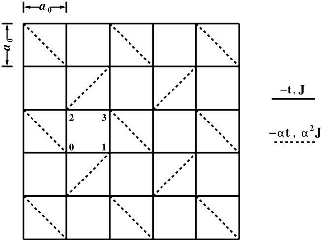
Figure 3: The Shastry-Sutherland lattice. Also shown is the labeling of sites in a unit cell of SS lattice, as used in the text.

The $t-J$ type model, thus arrived at is an appropriate generalization of the original SS model, in order to deal with doping. In the following, we will first describe the tight binding band structure of the free electrons on the SS lattice. Then, we will do the mean field theory of the interacting model and discuss its implications for superconductivity, in a manner analogous to the early RVB mean field theories of $t-J$ model on a square lattice done in the context of high-T_C superconductivity[25, 26].

The band-structure :

The SS lattice has a periodicity of $2a_{o}$, both along $\hat{\mbox{x}}$ as well as $\hat{\mbox{y}}$ directions, where $a_{o}$ is the lattice constant. With each site contributing just one relevant orbital, the tight-binding model on SS lattice is described by a four band hamiltonian given below.

$$H_{t}=\sum_{{\bf k},\sigma}\left[c_{0}^{\dagger}({\bf k})\;\;c_{1}^{\dagger}({\bf k})\;\;c_{2}^{\dagger}({\bf k})\;\;c_{3}^{\dagger}({\bf k})\right]_{\sigma}{\bf T(k)}\left[\begin{array}[]{c}c_{0}({\bf k})\\ c_{1}({\bf k})\\ c_{2}({\bf k})\\ c_{3}({\bf k})\end{array}\right]_{\sigma}$$ (3)

Here, $\sigma=\uparrow$ or $\downarrow$, and the wave-vector, ${\bf k}=(k_{x},k_{y})$, is such that $\frac{-\pi}{2a_{o}}\leq k_{x},k_{y}\leq\frac{\pi}{2a_{o}}$. The subscripts, $0,1,2,3$, refer to four different site within a unit cell. The dispersion matrix, ${\bf T(k)}$, is a $4\times 4$ hermitian matrix as given below.

$${\bf T(k)}=-t\left[\begin{array}[]{cccc}0&2\;$cos$(k_{x}a_{o})&2\;$cos$(k_{y}a_{o})&\alpha\;$e$^{i(k_{x}-k_{y})a_{o}}\\ 2\;$cos$(k_{x}a_{o})&0&\alpha\;$e$^{i(k_{x}+k_{y})a_{o}}&2\;$cos$(k_{y}a_{o})\\ 2\;$cos$(k_{y}a_{o})&\alpha\;$e$^{-i(k_{x}+k_{y})a_{o}}&0&2\;$cos$(k_{x}a_{o})\\ \alpha\;$e$^{-i(k_{x}-k_{y})a_{o}}&2\;$cos$(k_{y}a_{o})&2\;$cos$(k_{x}a_{o})&0\end{array}\right]$$ (4)

The band-structure for $|\alpha|=1.25$ is shown in Fig.(4). This value of $\alpha$ is taken from the studies on SrCu₂(BO₃)₂, where the values of $J$ and $J^{\prime}$ are extracted by fitting the experimental data with the orthogonal dimer model. What is known from the experiments is $\alpha^{2}$, and not $\alpha$. This leaves us with the ambiguity of sign of $\alpha$, and hence we have considered both positive as well negative values of $\alpha$.

Figure 4: The band-structure of free electrons on the SS lattice. The wave vectors are written in units of $\frac{1}{a_{o}}$. Notice that the band-structure is odd with respect to $\alpha$.

Let us make a few essential observations regarding the band-structure. Firstly, the system is a semi-metal at half filling, since the middle two bands touch each other at the zone centre. Secondly, there is a band which is flat along the X$\Gamma$ symmetry direction in the Brillouin Zone. This band gives rise to a severe van Hove singularity at $\alpha$. Thirdly, the values of band energies at zone centre are $(-4-\alpha)$, $\alpha$, $\alpha$ and $(4-\alpha)$. For $|\alpha|>2$, the middle two bands no more touch each other, and there is a finite band gap which makes it a band insulator at half filling. Since $\alpha$ for the material of real interest is roughly 1.25, we have not tried to discuss other values of $\alpha$.

Fig.(5) shows the non-interacting single particle density of states on SS lattice for both negative as well positive values of $\alpha$. When we hole-dope the system to take it away from half filling, it is expected to behave differently for positive and negative $\alpha$, since the flat band influences the case only when $\alpha$ is negative.

Figure 5: The density of single-particle electronic states on Shastry-Sutherland lattice.

The mean field hamiltonian :

The $t-J$ hamiltonian on SS lattice can be written as:

$$\tilde{H}={\cal P}H_{t}{\cal P}+H_{J}-t\mu\sum_{{\bf k},\sigma}\sum_{p=0}^{3}c_{p,\sigma}^{\dagger}({\bf k})c_{p,\sigma}({\bf k})$$ (5)

The first term in $\tilde{H}$ accounts for the projected hopping. It is essentially $H_{t}$ as given in equation(3), but with projection operator ${\cal P}$ which suppresses the double occupancy of any site (due to large Hubbard $U$). At a simple level, the effect of ${\cal P}$ can be brought in by replacing $t$ by $\delta t$. Here, $\delta(=1-n)$, is the number of holes per site, and $n$ is the electron filling per site. The last term is the chemical potential, $\mu t$, times the total number of electrons. Here, $p$ is the site (or the orbital) label within a unit cell. The second term in equation(5), $H_{J}$, which accounts for the interaction among electrons can be written as:

$$H_{J}=J\left\{\sum_{n.n.}+\;\;\alpha^{2}\sum_{n.n.n.}^{\prime}\right\}\left({\bf S(r)}\cdot{\bf S(r^{\prime})}-\frac{\hat{\mbox{n}}({\bf r})\hat{\mbox{n}}({\bf r}^{\prime})}{4}\right)$$ (6)

Here, ${\bf r}$ and ${\bf r^{\prime}}$ are the site labels, and $\hat{\mbox{n}}(\bf r)$ denotes the number operator at site ${\bf r}$. The summation is pairwise in ${\bf r}$, ${\bf r^{\prime}}$. The primed summation denotes the sum of only those pairs of n.n.n. sites which are allowed by the connectivity of the SS lattice. The operator, $\left({\bf S(r)}\cdot{\bf S(r^{\prime})}-\hat{\mbox{n}}({\bf r})\hat{\mbox{n}}({\bf r}^{\prime})/4\right)$, can also be written as $-\frac{1}{2}{\bf b^{\dagger}(r,r^{\prime})}{\bf b(r,r^{\prime})}$, which provides the basis for mean field decoupling of $H_{J}$ in the off-diagonal channel. The operator, ${\bf b(r,r^{\prime})}=c_{\downarrow}({\bf r})c_{\uparrow}({\bf r}^{\prime})-c_{\uparrow}({\bf r})c_{\downarrow}({\bf r}^{\prime})$, is the singlet bond operator.

Let us define an off-diagonal or the pairing mean field, $\left<{\bf b(r,r^{\prime})}\right>$, in the following way.

$$\left<{\bf b(r,r^{\prime})}\right>=\left\{\begin{array}[]{ll}\Delta$e$^{i\theta_{x}}&\;\;\;\;\mbox{for}\;\;{\bf r-r^{\prime}}=\pm a\hat{\mbox{x}}\\ \Delta$e$^{i\theta_{y}}&\;\;\;\;\mbox{for}\;\;{\bf r-r^{\prime}}=\pm a\hat{\mbox{y}}\\ \Delta^{\prime}$e$^{i\theta_{x+y}}&\;\;\;\;\mbox{for}\;\;{\bf r-r^{\prime}}=\pm a(\hat{\mbox{x}}+\hat{\mbox{y}})\\ \Delta^{\prime}$e$^{i\theta_{x-y}}&\;\;\;\;\mbox{for}\;\;{\bf r-r^{\prime}}=\pm a(\hat{\mbox{x}}-\hat{\mbox{y}})\end{array}\right.$$ (7)

The phases, $\theta_{x}$, $\theta_{y}$, $\theta_{x+y}$ and $\theta_{x-y}$, as well as the amplitudes, $\Delta$ and $\Delta^{\prime}$, are all independent of the coordinates. Hence, we are considering a uniform case. With this choice of the order parameter, we decouple $H_{J}$. The corresponding mean field hamiltonian can be written as:

$$\tilde{H}^{MF}=\tilde{H}_{t}+H_{J}^{MF}+L(4J\Delta^{2}+J^{\prime}{\Delta^{\prime}}^{2})$$ (8)

where $L$ is the number of unit cells. In order to write $\tilde{H}_{t}$ and $H_{J}^{MF}$ conveniently, we introduce a notation. Let us define the Nambu operators, $\Psi_{C\uparrow}({\bf k})$ and $\Psi_{R\downarrow}({\bf-k})$ in the following way.

$$\Psi_{C\uparrow}({\bf k}) = \left[\begin{array}[]{c}c_{0\uparrow}({\bf k})\\ c_{1\uparrow}({\bf k})\\ c_{2\uparrow}({\bf k})\\ c_{3\uparrow}({\bf k})\end{array}\right]$$ (13)

$$\Psi_{R\downarrow}(-{\bf k}) = \left[c_{0\downarrow}(-{\bf k})\;\;c_{1\downarrow}(-{\bf k})\;\;c_{2\downarrow}(-{\bf k})\;\;c_{3\downarrow}(-{\bf k})\right]$$ (14)

The subscripts, $C$ and $R$, indicate that $\Psi_{C\uparrow}({\bf k})$ is a column vector and $\Psi_{R\downarrow}({\bf-k})$ is a row vector. In this notation, $\tilde{H}_{t}$ can be written as :

$$\tilde{H}_{t}=\sum_{\bf k}\left\{\mbox{tr}\left\{{\bf\tilde{T}(-k)}\right\}+\left[\Psi^{\dagger}_{C\uparrow}({\bf k})\;\;\Psi_{R\downarrow}(-{\bf k})\right]\left[\begin{array}[]{cc}{\bf\tilde{T}(k)}&{\bf 0}\\ {\bf 0}&-{\bf\tilde{T}(k)}\end{array}\right]\left[\begin{array}[]{c}\Psi_{C\uparrow}({\bf k})\\ \Psi^{\dagger}_{R\downarrow}(-{\bf k})\end{array}\right]\right\}$$ (15)

Here, ${\bf\tilde{T}(k)}$ is essentially same as the dispersion matrix, ${\bf T(k)}$, except that the chemical potential forms its diagonal elements, and all the off-diagonal entries have a factor of hole doping, $\delta$, in order to account for the projection.

$${\bf\tilde{T}(k)}=-t\left[\begin{array}[]{llll}\mu&2\delta\;$cos$(k_{x}a_{o})&2\delta\;$cos$(k_{y}a_{o})&\delta\alpha\;$e$^{i(k_{x}-k_{y})a_{o}}\\ 2\delta\;$cos$(k_{x}a_{o})&\mu&\delta\alpha\;$e$^{i(k_{x}+k_{y})a_{o}}&2\delta\;$cos$(k_{y}a_{o})\\ 2\delta\;$cos$(k_{y}a_{o})&\delta\alpha\;$e$^{-i(k_{x}+k_{y})a_{o}}&\mu&2\delta\;$cos$(k_{x}a_{o})\\ \delta\alpha\;$e$^{-i(k_{x}-k_{y})a_{o}}&2\delta\;$cos$(k_{y}a_{o})&2\delta\;$cos$(k_{x}a_{o})&\mu\end{array}\right]$$ (16)

With the same notation, $H_{J}^{MF}$ can be written as :

$$H_{J}^{MF}=\left[\Psi_{C\uparrow}^{\dagger}({\bf k})\;\;\Psi_{R\downarrow}(-{\bf k})\right]\left[\begin{array}[]{cc}{\bf 0}&{\bf D(k)}\\ {\bf D^{\dagger}(k)}&{\bf 0}\end{array}\right]\left[\begin{array}[]{c}\Psi_{C\uparrow}({\bf k})\\ \Psi_{R\downarrow}^{\dagger}(-{\bf k})\end{array}\right]$$ (17)

where ${\bf D(k)}$ is a non-hermitian $4\times 4$ matrix as given below.

$${\bf D(k)}=-\left[\begin{array}[]{llll}0&J\Delta$e$^{i\theta_{x}}$cos$(k_{x}a_{o})&J\Delta$e$^{i\theta_{y}}$cos$(k_{y}a_{o})&\frac{J^{\prime}\Delta^{\prime}}{2}$e$^{i\theta_{x-y}}$e$^{i(k_{x}-k_{y})a_{o}}\\ J\Delta$e$^{i\theta_{x}}$cos$(k_{x}a_{o})&0&\frac{J^{\prime}\Delta^{\prime}}{2}$e$^{i\theta_{x+y}}$e$^{i(k_{x}+k_{y})a_{o}}&J\Delta$e$^{i\theta_{y}}$cos$(k_{y}a_{o})\\ J\Delta$e$^{i\theta_{y}}$cos$(k_{y}a_{o})&\frac{J^{\prime}\Delta^{\prime}}{2}$e$^{i\theta_{x+y}}$e$^{-i(k_{x}+k_{y})a_{o}}&0&J\Delta$e$^{i\theta_{x}}$cos$(k_{x}a_{o})\\ \frac{J^{\prime}\Delta^{\prime}}{2}$e$^{i\theta_{x-y}}$e$^{-i(k_{x}-k_{y})a_{o}}&J\Delta$e$^{i\theta_{y}}$cos$(k_{y}a_{o})&J\Delta$e$^{i\theta_{x}}$cos$(k_{x}a_{o})&0\end{array}\right]$$ (18)

Here, $J^{\prime}=\alpha^{2}J$ as mentioned earlier. Finally, we write the $\tilde{H}^{MF}$ as :

$$\tilde{H}^{MF} = \sum_{\bf k}\left[\Psi_{C\uparrow}^{\dagger}({\bf k})\;\;\Psi_{R\downarrow}(-{\bf k})\right]\left[\begin{array}[]{cc}{\bf\tilde{T}(k)}&{\bf D(k)}\\ {\bf D^{\dagger}(k)}&-{\bf\tilde{T}(k)}\end{array}\right]\left[\begin{array}[]{c}\Psi_{C\uparrow}({\bf k})\\ \Psi_{R\downarrow}^{\dagger}(-{\bf k})\end{array}\right]$$ (24)

$$+L\left(4J\Delta^{2}+J^{\prime}{\Delta^{\prime}}^{2}-4t\mu\right)$$

Let us denote the matrix $\left[\begin{array}[]{cc}{\bf\tilde{T}(k)}&{\bf D(k)}\\ {\bf D^{\dagger}(k)}&-{\bf\tilde{T}(k)}\end{array}\right]$ by A(k). It is an $8\times 8$ symplectic, hermitian matrix whose eigenvalues are real and occur in pairs. That is, an eigenvalue’s negative is also an eigenvalue.

The mean field free energy and the self-consistent equations :

The grand canonical free energy, $\Phi$, at a given temperature $T$, for the mean field hamiltonian described above is,

$$\Phi=4L\left(J\Delta^{2}+\frac{J^{\prime}{\Delta^{\prime}}^{2}}{4}-t\mu\right)-\sum_{\bf k}\sum_{j=1}^{4}\left\{E_{j}^{+}({\bf k})+\frac{2}{\beta}\mbox{Log}\left(1+\mbox{e}^{-\beta E_{j}^{+}({\bf k})}\right)\right\}$$ (25)

Here, $\beta=1/\mbox{k}_{B}T$, and $\left\{E_{j}^{+}({\bf k}),j=1,4\right\}$ are the positive eigenvalues of ${\bf A(k)}$. Let us put $t=1$. Now, all the energies (or parameters with units of energy) are in the units of $t$. We find the self-consistent equations for $\Delta$ and $\Delta^{\prime}$ by minimizing $\Phi$ with respect to $\Delta$ and $\Delta^{\prime}$. These are as follows.

$$\Delta = \frac{1}{2J}\frac{1}{4L}\sum_{\bf k}\sum_{j=1}^{4}\frac{\partial E_{j}^{+}({\bf k})}{\partial\Delta}\mbox{tanh}\left(\frac{\beta E_{j}^{+}({\bf k})}{2}\right)$$ (26)

$$\Delta^{\prime} = \frac{2}{J^{\prime}}\frac{1}{4L}\sum_{\bf k}\sum_{j=1}^{4}\frac{\partial E_{j}^{+}({\bf k})}{\partial\Delta^{\prime}}\mbox{tanh}\left(\frac{\beta E_{j}^{+}({\bf k})}{2}\right)$$ (27)

Since $\partial\Phi/\partial\mu=-N$, where $N$ is the total number of electrons, we get the following equation for the chemical potential.

$$\delta=-\frac{1}{4L}\sum_{\bf k}\sum_{j=1}^{4}\frac{\partial E_{j}^{+}({\bf k})}{\partial\mu}\mbox{tanh}\left(\frac{\beta E_{j}^{+}({\bf k})}{2}\right)$$ (28)

The hole doping, $\delta=1-N/4L$. Solving these sets of equations self-consistently gives us $\Delta$, $\Delta^{\prime}$ and $\mu$ as a function of $\delta$, for given values of $\alpha$, $J$, $\beta$ and the phase angles $\theta_{x}$ etc.

The results of the mean field theory :

We solve equations (26), (27) and (28) self-consistently for different values of $\delta$. We are interested in both the hole as well as electron doping for a given $\alpha$. It is clear from the band structure that the hole doping for $\alpha$ is same as the electron doping for $-\alpha$. Therefore, we have considered only the hole doping for both positive as well as negative $\alpha$. In all our computations, we use $t=1$, $J=0.3$ and $|\alpha|=1.25$. The value of $J$ for SrCu₂(BO₃)₂ is roughly 70⁰K. The ratio of $J$ to $t$ is tentative, and taken to be roughly same as that for the high-T_C superconductors. Though we have four phases, $\theta_{x}$, $\theta_{y}$, $\theta_{x+y}$ and $\theta_{x-y}$, only three relative phases are relevant. Therefore, we keep $\theta_{x}=0$. We have to find out those values of $\theta_{y}$ etc. for which the free energy is minimized, and see how things evolve as a function of $\delta$.

Let us discuss the zero temperature ($\beta\rightarrow\infty$) case first. Fig.(6) shows the variation of $\Delta$ and $\Delta^{\prime}$ with respect to $\delta$, for $\alpha=-1.25$ and 1.25 at zero temperature. For $\alpha=-1.25$, the minimum of free energy occurs for $\theta_{x+y}-\theta_{x-y}=\pi$ regardless of the values of $\theta_{x}$ and $\theta_{y}$, and $\Delta$ is identically zero. For $\alpha=1.25$, the minimum of free energy corresponds to $\theta_{x}=0$, $\theta_{y}=\pi$, $\theta_{x+y}=0$ and $\theta_{x-y}=\pi$. It is a weak minimum as many other choices of the phases have similar values of the free energy. Nevertheless, this choice of phases appears to be the minimum. It is interesting to note that for $\delta=0$, the diagonal bond order parameter, $\Delta^{\prime}$, is one and $\Delta$ is zero (and is independent of the phases $\theta_{x}$, $\theta_{y}$, $\theta_{x+y}$ and $\theta_{x-y}$). Thus, the RVB mean field theory at half filling exactly reproduces the known dimer ground state of the SS model.

Figure 6: The variation of $\Delta$ and $\Delta^{\prime}$ with doping, $\delta$, in the ground state. For $\alpha=-1.25$, $\Delta$ is not shown, since it is identically zero.

To consider superconductivity in our mean field theory, we define a physical order parameter, $\Delta_{\rm SC}=F_{B}\Delta_{\rm MF}$. Here, $\Delta_{\rm MF}$ is the mean-field order parameter ($\Delta$ or $\Delta^{\prime}$ whichever is larger for a given doping), and $F_{B}$ is a bosonic mean field. Such an order parameter can be understood in the framework of slave boson approach[27], where the off-diagonal order parameter of the physical electrons is described as $\left<b_{i}b_{j}f_{i\sigma}^{\dagger}f_{j{\sigma^{\prime}}}^{\dagger}\right>$. Here $b$’s are the slave boson fields, and $f$’s are the fermionic objects. In a mean field decoupled theory, this is like $\left<b_{i}b_{j}\right>\left<f_{i\sigma}^{\dagger}f_{j{\sigma^{\prime}}}^{\dagger}\right>\equiv F_{B}\Delta_{\rm MF}$. The bosonic order parameter, $F_{B}$, is a function of temperature and doping, and goes roughly like $\delta$. The superconducting transition temperature, T_SC, is the temperature where either $\Delta_{\rm MF}$ or $F_{B}$ vanishes first while increasing the temperature. For low doping, $\Delta_{\rm MF}$ is large, therefore, the T_SC is same as the bose condensation temperature, T_BC, for the bosonic field. Some estimates of T_BC have been made earlier while studying $t-J$ model in the context of the high-T_C superconductivity[27]. We roughly estimate it by considering an approximate dispersion of the form, $k_{x}^{2}+k_{y}^{2}+\frac{1}{\gamma}k_{z}^{2}$, with the z-axis anisotropy $\gamma\sim 30$. We get T${}_{\rm BC}\approx 4\pi\rho^{*}\delta(1-\delta)/[2+$Log$(4\gamma/\pi)]$. Here, $\rho^{*}$ is the density of states at the energy where two middle bands touch, from the side where dispersion is quadratic, and is a measure of the curvature of the band. For $|\alpha|=1.25$, $\rho^{*}\approx 0.1$, thus T${}_{\rm BC}\approx 0.22\delta(1-\delta)$.

One comment should be made regarding the interpretation of the result $\Delta=0$ and $\Delta^{\prime}\neq 0$ (for $\alpha<0$). While at half filling this implied the dimerized insulating state, away from half filling it must be interpreted as superconductivity. The BCS type wavefunction implies the fermion pairing in real space,

$$\left<c_{i\uparrow}^{\dagger}c_{j\downarrow}^{\dagger}\right>\sim\sum_{\bf k}\mbox{e}^{i{\bf k}\cdot(\mbox{\bf r}_{i}-\mbox{\bf r}_{j})}\frac{\Delta_{\bf k}}{\sqrt{\Delta_{\bf k}^{2}+(\epsilon_{\bf k}-\mu)^{2}}}\;\;,$$

and it extends over a range of lattice constants (due to the non-trivial k dependence of $\epsilon_{\bf k}$ away from $\delta=0$), despite the mean field Hamiltonian having $n.n.$ pairing only. A similar remark holds for the four fermi operator that determines the superconducting ODLRO of Yang, namely $\left<c_{i\uparrow}^{\dagger}c_{j\downarrow}^{\dagger}c_{j^{\prime}\downarrow}c_{i^{\prime}\uparrow}\right>\neq 0$ for $|\mbox{\bf r}_{i}-\mbox{\bf r}_{j}|>>1$.

Fig.(7) shows the phase diagram in the T-$\delta$ plane, as estimated from our RVB mean field theory. The temperature, T_MF, is where $\Delta_{\rm MF}$ vanishes. The estimated T_BC, and the computed T_MF are plotted as a function of $\delta$. The common region under these two curves is the superconducting phase bounded by critical lines. As usual all the remining lines should be viewed as crossover lines rather than critical lines. Among the remaining three regions of T-$\delta$ phase diagram, the low doping region below T_MF and above T_BC is the spin gap phase with a suppressed density of states manifested in susceptibility as well as optical conductivity. Similarly, the high doping region is the normal fermi liquid. There is a region which is usually referred to as the strange metal phase, as shown in the Fig.(7) with linear resistivity. Also, the phase diagram is similar for both positive as well negative values of $\alpha$. From this phase diagram, we estimate the optimal value of the superconducting transition temperature, T${}_{C}\sim 10^{0}$K.

Figure 7: The phase diagram for the negative as well positive values of $\alpha$. The lines of the estimated Bose condensation temperature, T_BC, and the computed mean field temperature, T_MF, divide the T-$\delta$ plane into four physically distinct regions. Each of these is appropriately labeled.

In conclusion, the system considered here has a rather rich history. It may also have an important future since under doping it might be the much sought after low $T_{c}$ RVB superconductor, with linear resistivity down to 10 K and other such exotic properties, rather than a conventional phononic BCS superconductor.

3 Acknowledgements

BSS would like to thank the organizers of the Nishinomiya Yukawa Symposium for the warm hospitality. He thanks Professors E. Abrahams, P. Nozières, M. Schlüter, H. Kageyama, K. Ueda and J. Goplakrishnan for useful discussions spread over various years.

^†Article based on an invited talk given by BSS at the 16th Nishinomiya Yukawa memorial symposium on “ Order and Disorder in Quantum Spin Systems”, Nov 13-14, 2001 at Nishinomiya.

^∗ The mean field theory of the doped dimer in Section 2. is joint work with B Kumar.

References

- [1] B S Shastry and B. Sutherland, Physica B 108, 1069 (1981)
- [2] M E Fisher, in Summary talk at the 1992 USA Japan meeting at the Institute of Theoretical Physics, Santa Barbara. Professor Fisher emphasized here and elsewhere, the crucial role played by the two dimensional Ising model solution of Onsager in the development of the theory of critical phenomena. Our colleague at IISc, Professor Chandan Dasgupta, has remarked in a similar vein that, if not for Baxters solution of the two dimensional q state Potts model order parameter, a truly subtle object, we might even today be debating the order of the phase transition in the system.
- [3] B Sutherland and B S Shastry, J. Stat. Phys. 33, 477 (1983).
- [4] S. Miyahara and K. Ueda, Phys. Rev. Lett 82, 3701 (1999), (2000) cond-mat /0004260.
- [5] C Knetter, A Bühler, E Müller-Hartmann and G Uhrig, Phys Rev Lett 85 3858 ( 2000).
- [6] H Kageyama, M Nishi et al, Phys Rev Lett 84 5876 (2000)
- [7] H Kageyama, K Yoshimura et al, Phys Rev Lett 823168 ( 1999).
- [8] H Nojiri et al, J Phys Soc Japan 68 2906 ( 1999).
- [9] P Lemmens et al, Phys Rev Lett 85 2605 (2000).
- [10] M Hoffmann et al, Phys Rev Lett 87 047202 ( 2001).
- [11] K Totsuka, S Miyahara and K Ueda, Phys Rev Lett 86 520 ( 2001), Y Fukumoto, cond-mat/000411 (2000).
- [12] K Onizuka et al, J Phys Soc Japan 69, 1016 ( 2000).
- [13] Y Fukumoto, cond-mat/0012396, T Momoi and K Totsuka, Phys Rev 62 15067 ( 2000),
- [14] G Misguich, Th Jolicoeur and S Girvin, Phys Rev Lett 87 097203 ( 2001).
- [15] A Koga and N Kawakami , Phys Rev Lett 84 4461 ( 2000), cond-mat/0003435 (2000).
- [16] Z Weihong, J Oitmaa and C Hamer, cond-mat/0107019 ( 2001).
- [17] U Löw and E Müller-Hartmann, cond-mat/0104385 ( 2001).
- [18] C Chung, J Marston and S Sachdev, Phys Rev 64 134407 ( 2001).
- [19] D Carpentier and L Balents, cond-mat/0102218 ( 2001).
- [20] M Albrecht and F Mila, Europhys Lett 34 145 ( 1996).
- [21] N Surendran and R Shankar, cond-mat/0112507 ( 2001),
- [22] E Müller-Hartmann, R R P Singh, C Knetter and G Uhrig, Phys Rev Lett 84 1808 ( 2000).
- [23] We owe this comment to Professor P Nòzieres.
- [24] J Nagamatsu, N Nakagawa, T Muranaka, YZenitani and J Akimitsu, Nature, 410 63, (2001), J Kortus, I I Mazin, K D Belashchenko, V P Antropov and L L Boyer,cond-mat/011446
- [25] G. Baskaran, Z. Zou and P. W. Anderson, Solid State Commun. 63, 973 (1987)
- [26] G. Kotliar and J. Liu, Phys. Rev. B 38, 5142 (1988)
- [27] M. U. Ubbens and P. A. Lee, Phys. Rev. B 49, 6853 (1994)