Scaling in self-organized criticality from interface depinning?

Abstract

The avalanche properties of models that exhibit ’self-organized criticality’ (SOC) are still mostly awaiting theoretical explanations. A recent mapping (Europhys. Lett. 53, 569) of many sandpile models to interface depinning is presented first, to understand how to reach the SOC ensemble and the differences of this ensemble with the usual depinning scenario. In order to derive the SOC avalanche exponents from those of the depinning critical point, a geometric description is discussed, of the quenched landscape in which the ’interface’ measuring the integrated activity moves. It turns out that there are two main alternatives concerning the scaling properties of the SOC ensemble. These are outlined in one dimension in the light of scaling arguments and numerical simulations of a sandpile model which is in the quenched Edwards-Wilkinson universality class.

I Introduction

The concept of reaching “self-organized” criticality (SOC) in a model without any apparent tuning parameter draws still attraction AIP . In many real-life systems power-law probability distributions are met, and it is thus an obvious question to ask why they would resemble ordinary critical phenomena. To this end, sandpile models have been the prevalent theoretical playground for the last fifteen years. Only recently their understanding has finally started to take shape. Two supporting approaches have been developed. The crucial notion is that the critical state in these models draws from both the boundary conditions and the drive, and also has a generic, field-theoretical description. This can be formulated as a variant of the directed percolation-style Reggeon field theory (RFT) guys , or as a mapping to interface depinning ala1 ; ala2 ; ala3 ; previous . The gist of this mapping is based on the description of the history of the sandpile model and its dynamics via a stochastic differential equation, the quenched Edwards-Wilkinson (qEW) equation qew1 ; qew2 . Likewise a suitable RFT for sandpiles includes by necessity a density conserving term that accounts for the effects of diffusional transport of particles or grains.

In this article the description of sandpiles through interface depinning is reviewed. The issue of particular interest to us is the physics of driven interfaces that describe sandpile models. To this end Section II introduces in a short fashion the mapping, and discusses the ensemble in which SOC is reached. It is seen that this is not any of the normal ones familiar in the context of the qEW, say. The next section is devoted to a discussion of the standard properties of interface scaling at the depinning transition, and, correspondingly, the scaling laws usually formulated for sandpiles depending on the ensemble. We next concentrate in particular on a geometric description of depinning. This is the essential issue in obtaining the scaling exponents of SOC avalanches: the extension of the theory of ’elastic pinning paths’ to the SOC case. In section IV numerical results are considered for the one-dimensional qEW sandpile in the SOC ensemble. This is the simplest model system in which one can try to extract a correspondence with the avalanche and the depinning pictures. This is since the 1D pinning paths can be discussed without the introduction of extra, independent exponents. Finally, section V finishes the paper with a summary about SOC properties based on recent advances including the numerical work presented here, and about remaining open problems.

II Mapping sandpiles to interfaces

Consider a sandpile model with each site $x$ of a hyper-cubic lattice having $z(x,t)$ grains. When $z(x,t)$ exceeds a critical threshold $z_{c}(x)$, the site is active and topples so (y is a nearest neighbour of $x$)

$$z(x,t+1)=z(x,t)-2d,~{}z(y,t+1)=z(y,t)+1.$$ (1)

$z_{c}(x)$ is taken to be a random variable, chosen from a probability distribution $P(z_{c})$ again after each toppling. If there are no active sites in the system, one grain is added to a randomly chosen site, $z(x,t)\to z(x,t)+1$. This is the SOC ensemble, defined via the drive and the open boundaries, characterized by avalanches that may ensue after a grain has been deposited. The dynamics of this model can be reinterpreted through an ’interface’, or history $H(x,t)$ which follows the memory of all the activity at $x$. $H$ counts topplings at site $x$ up to time $t$, and has the dynamics

$$H(x,t+1)=\left\{\begin{array}[]{ll}H(x,t)+1,&f(x,t)>0,\\ H(x,t),&f(x,t)\leq 0,\end{array}\right.$$ (2)

This can be written as a discrete interface equation

$$\frac{\Delta H}{\Delta t}=\theta\left(f(x,t)\right),$$ (3)

with $\theta(f)$ the step-function forcing it so that the interface does not move backwards. The ’local force’ is

$$f(x,t)=z(x,t)-z_{c}(x)=n_{x}^{in}-n_{x}^{out}-z_{c}(x),$$ (4)

in terms of $n_{x}^{in}$ (grains added to site $x$ up to time $t$) and $n_{x}^{out}$ (grains removed from $x$). The fluxes $n_{x}^{in}$ and $n_{x}^{out}$ can be worked out in terms of the local height field $H(x,t)$, and a columnar force term $F(x,t)$ which counts the number of grains added to site $x$ by the external drive,

$$f(x,t)=\nabla^{2}H+F(x,t)-z_{c}(x,H).$$ (5)

The step-function, $\theta(f)$, in Equation (3), the condition that the interface does not move backwards, introduces an extra noise term $\sigma(x,H)$ - the velocity of the interface is either one or zero - but for the current example this should not be relevant. Combining the three sources of effective noise, $F$, $z_{c}$ and $\sigma$, one ends at the discretized interface equation

$$\frac{\Delta H}{\Delta t}=\nabla^{2}H+\eta(x,H)+F(x,t)+\sigma(x,H).$$ (6)

Here the quenched noise $\eta(x,H)=-z_{c}(x,H)$, and we have obtained the central difference discretization of a continuum diffusion equation with quenched noise, called the linear interface model (LIM) or the quenched Edwards-Wilkinson equation qew1 ; qew2 . The continuum limit reads $\partial_{t}h(x,t)=\nu\nabla^{2}h(x,t)+F+\eta(x,h(x,t))$.

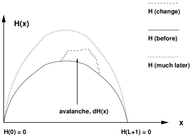
Figure 1: One-dimensional schematic example of the interface or history representation of a SOC sandpile model. The mean-field interface follows an average parabolic shape, which also implies that in the SOC steady-state $v(x)$ is parabolic. Notice the boundary conditions $H=0$ that ensure the loss of particles (equalling the increased elastic energy) in that state.

The SOC ensemble is illustrated in Figure (1). Once the local force is increased, by adding a grain and making $F(x,t)\rightarrow F(x,t)+1$ at the chosen $x$ an avalanche starts since the force overcomes the pinning force, $\nabla^{2}H+\eta(x,H)+F(x,t)>0$. The interface moves at $x$ by one step, $\Delta H(x)=1$. In the subsequent dynamics of the avalanche the columnar force term $F(x)$ does not change. For the SOC sandpiles, the correct choice of the interface boundary condition is $H=0$ which is to be imposed at two “extra sites” ($x=0$, $x=L+1$ for a system of size $L$ in 1D). The ever-increasing $\langle F(t)\rangle$ leads to an average parabolic interface shape via the cancellation of the Laplacian by $F$. It is to be stressed that this implicitly contains the physics of the SOC state: the driving force $F(x,t)$ is increased so slowly that the avalanches do not overlap and are therefore well-defined ala1 .

III Scaling properties of ensembles

Equation (6) exhibits a depinning transition at a threshold force $F_{c}$ in a normal ensemble. The interface configuration and dynamics develop critical correlations in the vicinity of the critical point. For the case of point-correlated disorder the normal way to analyze the LIM is to use the functional renormalization group method. One-loop expressions for the exponents are found in papers by Nattermann et al., Narayan and Fisher qew1 ; qew2 , and in the more recent ones by Le Doussal and collaborators Doussal .

The problem is technically and from the fundamental viewpoint difficult, since the whole disorder correlator is renormalized. The point-random field noise term forms one of the universality classes in this problem qew1 ; qew2 ; others are the LIM with columnar noise columnar and the quenched Kardar-Parisi-Zhang equation TKD ; HHZ ; Barabasi ; Gabor in more general terms. The mapping of SOC models to variants of LIM holds however some surprises. For instance, while the conjecture that the Manna model manna should be in the usual point-disorder LIM class seems to be true in 2D, this is clearly not so in 1D if considered in the depinning ensemble mannarefs . The complications arise since an arbitrary choice of sandpile rules can lead to non-standard noise correlations that do not need to have a priori the same RG fixed point as the random field or force case.

In the interface language the relevant exponents to describe the depinning phase transition are: $\nu$ (the correlation length exponent), $z$ (the dynamical exponent), and $\chi$, the roughness exponent. Moreover assuming that the avalanche dynamics suffices to describe the interface dynamics off the critical point, $\theta=\nu(z-\chi)$ holds for the velocity exponent, with $v\sim(F-F_{c})^{\theta}$ qew2 ; qew1 . For point-like disorder the first-loop functional RG results cited above read $\chi=(4-d)/3$, and $z=2-(4-d)/9$. Notice the exponent relation $\nu=1/(2-\chi)$ which manifests together with the $\theta$-exponent relation the fact that there is only one temporal and one spatial scale at the critical point.

The typical quantity to be measured in the interface context is the interface width $w$ (mean fluctuation) which in most cases equals other measures like the two-point correlation functions and the structure factor Barabasi . From the sandpile viewpoint, these measure the correlations and fluctuations in the activity history, that is in the avalanche series. Initially the width grows, as a function of time, as $w\sim t^{\beta}$ defining the ’growth exponent’ $\beta$ until either saturation is reached (with a finite order parameter, $v$), or the interface gets pinned at or below $F_{c}$. Scaling now implies $\beta z=\chi$, as for general interface models.

The LIM obeys an important invariant, with the static response scaling as qew2 $\chi(q,\omega=0)\sim q^{-2}$, so that

$$\gamma/\nu=2.$$ (7)

For forces below $F_{c}$, the (bulk) response of the interface triggered by a small increase in $F$ is $\chi_{\rm bulk}\equiv{d\left<H\right>}/{dF}\sim(F_{c}-F)^{-\gamma}$. By assuming that the avalanche due to a point seed scales as $\Delta H\sim s\sim\ell^{D}$, $D={d+\chi}$ (since $H$ scales with the roughness as $\ell^{\chi}$), a hyperscaling relation can be derived for $\gamma$. Right at the critical point qew2 ; qew1 , the roughness of the interface scales as $\ell^{\chi}$ and assuming that $\Delta\left<H\right>$ will scale in the same way it follows

$$\gamma=1+\chi\nu.$$ (8)

This also implies $\chi+1/\nu=2$, as noted above. The standard scaling relations are valid for parallel dynamics: all sites with $\partial H/\partial t>0$ are updated in parallel. For extremal drive criticality (updating one unstable site at a time) the dynamic exponent reads $z_{\rm ED}=2$.

The 1D LIM is a bit more peculiar than one might expect. Numerics (which has recently been matched by the 2-loop RG results of LeDoussal et al.) implies that $\chi\sim 1.2\dots 1.25$ which is larger than the 1-loop and scaling argument result $\chi_{1d}=1$. The physical interpretation for the fact that $\chi>1$ has been dubbed “anomalous scaling” Lesch ; Juanma , and arises from a divergent mean height difference between neighboring sites, with $t\to\infty$.

The SOC steady-state is characterized by the probability to have avalanches of lifetime $t$ and size $s$ which follow power-law distributions: $p(t)=t^{-\tau_{t}}f_{t}(t/L^{z})$ and $p(s)=s^{-\tau}f(s/L^{D}),$ with $s\sim t^{D/z}$ and $z(\tau_{t}-1)=D(\tau-1)$. One can also characterize the avalanche by its linear dimension, $p(\ell)=\ell^{-\tau_{\ell}}f_{\ell}(\ell/L)$, with $\tau_{\ell}=1+D(\tau-1)$. Here the size scales as $s\sim\ell^{D}$ and the (spatial) area as $\ell^{d}$ (for compact avalanches) with $\ell$ the linear dimension. The fact that each added grain will perform of the order of $L^{2}$ Dhar topplings before leaving the system leads to the fundamental result

$$\left<s\right>\sim L^{2}$$ (9)

independent of dimension tang:1988 . Thus, $\tau=2-2/D$ and $\tau_{t}=1+(D-2)/z$. Equation (9) yields $\gamma/\nu=2$, where $\gamma$ describes the divergence of the susceptibility (bulk response to a bulk field) near a critical point, if one generalizes the exponent relation of the depinning ensemble to the SOC case. In the particular case of an increasing drive and a bulk dissipation, which induces a term $-kH$ to the qEW equation, this should, evidently, be valid bulk .

IV The one-dimensional QEW sandpile: geometric description of avalanches

To go beyond the scaling exponents to a description of the probability distributions at the critical point of any particular ensemble is a more challenging task. This is easiest in one dimension, which we thus discuss here. The most well-known case in which the geometry of the random quenched landscape allows to use a self-affine picture of the progress of an interface through it is given by directed percolation depinning (DPD), the quenched KPZ cousin of the qEW TKD ; HHZ ; Barabasi .

In this language the interface moves, e.g. in the case of an applied extremal drive, via a succession of punctuation events . The interface is assumed to invade the voids of a connected network in each of these events, in ’bursts’. In between these events, the pinned interface is mapped into a connected path on the backbone of a suitable (elastic) percolation problem pinningpaths , For DPD the analogy is more or less clear, and for the qEW one speaks of elastic pinning paths. Such paths have the characteristics that the RHS of the qEW is always negative semi-definite, ie. $f\leq 0$. It is not known rigorously whether such paths at criticality follow strictly the DPD -like scaling properties. There are two fundamental issues: the geometric properties of avalanches (the scaling of voids, or whether the relation of size vs. area can be characterized with a local roughness exponent $\chi_{loc}$) and the probability to induce an avalanche, or punctuation event if the interface is pushed at any particular spot (this issue is still open to discussion, see huber ; zeitak ; jost ).

Assuming that the DPD analogy works huber , it follows in the depinning ensemble for the avalanche size exponent

$$\tau_{s,dep}=1+(1/(1+\chi_{loc}))(1-1/\nu)$$ (10)

which using eg. the exponent relation $\nu=1/(2-\chi)$ and a reasonable value for $\chi_{loc}$, taken to equal the global $\chi$, produces

$$\tau_{s,dep}\approx 1.08.$$ (11)

For the SOC ensemble, the description of the critical state is given in terms of the avalanche distribution exponents - note that due to the inhomogeneity of the ensemble e.g. perturbing the system off the critical point is more complicated ala3 . One has then to ask the question what is the prediction of pinning-path picture. Due to the symmetries (static response) of the qEW it could be assumed that the typically parabolic interface profile is irrelevant, except perhaps for finite size corrections induced by the boundary condition that is imposed on the pinning paths since $H=0$ at the edges. This would imply, in particular, that for the SOC avalanche exponent it is found that

$$\tau_{s,SOC}\rightarrow\tau_{s,dep}.$$ (12)

A parallel approach is to use the invariant (9) which leads to the prediction

$$\tau_{s,SOC}=2-2/D=2-2/(1+\chi_{loc})$$ (13)

by using the roughness exponent to estimate the cut-off dimension of avalanches. This is identical with the pinning path estimate above.

These are then the major issues: is the depinning geometric description applicable to the SOC ensemble and if not why? The answer should depend only on fundamental similarities or differences between the ensembles, and not on the particular model - class of qEW-like models - nor the dimensionality. The study of the outcome is the easiest in 1D whereas in higher dimensions further independent exponents are needed, i.e. assumptions to describe the probability distributions since the avalanches have in addition to an area vs. volume relation also a perimeter length vs. area one higherdim ; zeitak .

To study the issue we next outline some numerical results on the 1D qEW/LIM, obtained from a Leschhorn-like cellular automaton Lesch ; jost for the interface problem. The system is run as a sandpile in that after the interface gets pinned a new avalanche initiation is done by increasing the local force $F_{i}$ at a random location by one. System sizes upto $L=8192$ have been studied, with 2 $\times$ 10⁶ avalanches for the largest sizes tobe . The resulting avalanche size distributions, after logarithmic binning, imply that the effective $\tau$-exponent varies with $L$, and that the weight of the power-law -like tail increases with the size. Meanwhile, the effective roughness exponent slightly decreases. Due to the systematic finite size corrections it does not make sense to try a normal datacollapse using a fixed $D$ and $\tau_{SOC}$ for all $L$. This is a little bit surprising given that relation (9) is fulfilled within numerical accuracy by the data, and that higher momenta of the size distributions indicate just simple scaling of the avalanche size distribution. Certainly more numerical analysis is called for, but two facts are worth pointing out. First, even for the largest system size the effective $\tau$ is way off from the predicted 1.08 (1.024 for $L=8192$). Second, by blindly - without any a priori justification - using the scaling Ansatz

$$\tau_{SOC}(L)=\tau_{SOC}(L=\infty)+\Delta\tau(L),$$ (14)

with a best-working function $\Delta\tau$, one observes that there is an apparent power-law correction to the exponent. This extrapolates very slowly in $L$ to $\tau_{SOC}(\infty)\sim 1.115$, ie. clearly off the depinning ensemble value. From $\tau_{SOC}$ it would be in principle possible to derive the other exponents as well, using the consequences of Eq. (9),

V Conclusions

Above, we have discussed a strategy to understand so-called self-organized criticality by mapping the history of a sandpile model to a driven interface in a random medium. For SOC models this idea is useful since it helps to understand universality classes (via noise terms generated) though there are theoretical challenges in the understanding of the possible classes (RG fixed points), and in the role of the discretization (called $\sigma$-noise above). Such work follows the historical connections of SOC to depinning, and extends it by explicitly constructing the right ensemble to reach SOC, and by outlining a general strategy to understand various models. Applied to other absorbing state phase transitions, in general, the history/interface description should be of interest. In some cases (e.g. the contact process) it can give rise to new, seemingly independent exponents dm .

Once one has defined the right ensemble for SOC in interface depinning, the most pertinent question becomes if the usual avalanche exponents in SOC can be derived from those of the depinning transition. Here we have addressed the question, but since the outcome is still open, it is worth reiterating the two possibilities. Either eventually, by studying large enough systems numerically, the exponents of the statistically homogeneous ensemble are recovered once finite size effects become negligible. Or, it becomes apparent that the SOC ensemble is an independent one. The microscopic reason for this would be that the density of grains (average force for the interface) is non-uniform: in one dimension it is easy to see that a site $x$ will get a larger grain flux from its neighbor on the bulk side and a smaller one from the boundary side - more trivially, there is a net flux of grains towards the boundaries. This inhomogeneity may persist in the thermodynamic limit, in which case the avalanche relations will be determined by its scaling properties.

Consider the idea depicted in Figure (3). The integral of the average force deviation at $x$, $\Delta F(x)=F_{dep}-F(x)_{SOC}$, where $F_{dep}$ and $F(x)_{SOC}$ are averages at the critical points of the ensembles, can be used to define a finite-size correction to the normal critical point, as $\int\Delta F(x)dx\equiv\delta F(L)$. It is seen that $\delta F$ will be dependent on the exact scaling function of $F(x)_{SOC}$, computing which is thus the crucial issue. It will give indirectly the true correlation length exponent $\nu_{SOC}$ in the SOC ensemble via the $L$-dependence of the finite size correction, which may or may not be the same as for the depinning case. The implication can be rephrased so that the usual exponents like $\nu$ are derived from the RG in an ensemble with statistical translational invariance in the $x$-direction. It is thus not obvious whether the properties of self-organized critical state actually follow from boundary -induced criticality or are related to the usual depinning one. In this respect the usual SOC models discussed here are inherently more complicated than the boundary driven cases like the so-called rice-pile model. This is in particular true if the symmetries of the depinning transition are broken by the SOC ensemble, as is the case for the quenched KPZ equation Gabor .

To summarize, the above problem is central in understanding SOC-like systems. It may also be tackled, perhaps, from the viewpoint of absorbing state phase transitions and their field-theoretical description which provides a parallel route to the interface one. There are many other interesting issues, like the early-stage dynamics (growth exponent $\beta$, suitably defined for the SOC ensemble), the question of the pinning path/manifolds in higher dimensions and so forth. For all these it is invaluable that one can resort to continuum descriptions of the SOC sandpiles, that also seem to be inter-connected, in an intriguing fashion alepp ; am .

ACKNOWLEDGMENTS

The results presented here have been in part obtained in an enjoyable collaboration with K. B. Lauritsen, M. Muńoz, R. Dickman, A. Vespignani, and S. Zapperi. The Academy of Finland’s Center of Excellence Program is thanked for financial support.

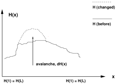
Figure 2: An avalanche at the critical point of the normal, translationally invariant, depinning ensemble . The statistical description of such avalanches follows the scaling law $\langle s\rangle=l^{1+\chi}$, where $l$ is (here in 1D) the area of the avalanche and $s$ its size.

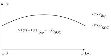
Figure 3: The average force per site, $\langle f(x)\rangle$ in the depinning and SOC ensembles. $\langle f\rangle$ is to be computed by computing the number of grains per site between the avanlanches.

References

- (1) See e.g. M. A. Muñoz, R. Dickman, R. Pastor-Satorras, A. Vespignani, and S. Zapperi, “Sandpiles and absorbing state phase transitions: recent results and open problems,” to appear in Procedings of the Granada seminar on computational physics, Ed. J. Marro and P. L. Garrido. (AIP 2001). e-print: cond-mat/0011447.
- (2) A. Vespignani, R. Dickman, M. A. Muñoz, and S. Zapperi, Phys. Rev. Lett. 81, 5676 (1998); R. Dickman, M. A. Muñoz, A. Vespignani, and S. Zapperi, Braz. J. Phys. 30, 27 (2000).
- (3) M. Alava and K. B. Lauritsen, Europhys. Lett. 53, 569 (2001); cond-mat/0002406.
- (4) K. B. Lauritsen and M. Alava, cond-mat/9903346.
- (5) M. Alava and K. B. Lauritsen, in preparation.
- (6) For previous work see O. Narayan and A. A. Middleton, Phys. Rev. B49, 244 (1994) for the case of the Bak-Tang-Wiesenfeld model (P. Bak, C. Tang, and K. Wiesenfeld, Phys. Rev. Lett. 59, 381 (1987)) in the depinning ensemble, only, and M. Paczuski and S. Boettcher, Phys. Rev. Lett. 77, 111 (1996) for the boundary-driven qEW.
- (7) T. Nattermann, S. Stepanow, L.-H. Tang, and H. Leschhorn, J. Phys. (France) II 2, 1483 (1992); H. Leschhorn, T. Nattermann, S. Stepanow, and L.-H. Tang, Ann. Physik 7, 1 (1997).
- (8) O. Narayan and D. S. Fisher, Phys. Rev. B48, 7030 (1993).
- (9) P. Chauve, P. Le Doussal, and K. J. Wiese, Phys. Rev. Lett. 86, 1785 (2001).
- (10) G. Parisi and L. Pietronero, Europhys. Lett. 16, 321 (1991); Physica A 179, 16 (1991).
- (11) L.-H. Tang, M. Kardar, and D. Dhar, Phys. Rev. Lett. 74, 920 (1995).
- (12) T. Halpin-Healy and Y.-C. Zhang, Phys. Rep. 254, 215 (1995).
- (13) A. -L. Barabási and H. E. Stanley, Fractal Concepts in Surface Growth, (Cambridge University Press, Cambridge, 1995).
- (14) G. Szabo, M.J. Alava, and J. Kertesz, submitted for publication.
- (15) S. S. Manna, J. Phys. A 24, L363 (1991).
- (16) See for the 2D case: A. Vespignani, R. Dickman, M. A. Muñoz, and S. Zapperi, Phys. Rev. E62, 4564 (2000); and for the 1D one R. Dickman, M. Alava, M. A. Muñoz, J. Peltola, A. Vespignani, and S. Zapperi, Phys. Rev. E64, 056104 (2001).
- (17) H. Leschhorn, Physica A 195, 324 (1993).
- (18) J. M. López and M. A. Rodríguez, Phys. Rev. E54, R2189 (1996); J. M. López, M. A. Rodríguez and R. Cuerno, Phys. Rev. E56, 3993 (1997).
- (19) D. Dhar, Phys. Rev. Lett. 64, 1613 (1990).
- (20) C. Tang and P. Bak, Phys. Rev. Lett. 60, 2347 (1988).
- (21) A. Barrat, A. Vespignani, S. Zapperi, Phys. Rev. Lett. 83, 1962 (1999) and references therein.
- (22) H. A. Makse et al., Europhys. Lett. 41, 251 (1998).
- (23) G. Huber, M.H. Jensen, and K. Sneppen, Phys. Rev. E52, R2133 (1995).
- (24) Z. Olami, I. Procaccia, and R. Zeitak, Phys. Rev. E52, 3042 (1995).
- (25) A.-L. Barabasi, G. Grinstein, and M. Muńoz, Phys. Rev. Lett. 76, 1481 (1996).
- (26) M. Jost, Phys. Rev. E57, 2634 (1998).
- (27) M. Alava, in preparation
- (28) R. Dickman and M. A. Muñoz, Phys. Rev. E 62, 7632 (2000).
- (29) M. Rossi, R. Pastor-Satorras, and A. Vespignani, Phys. Rev. Lett. 85, 1803 (2000); R. Pastor-Satorras and A. Vespignani, Phys. Rev. E62, R5875 (2000).
- (30) M.J. Alava and M.A. Muñoz, Phys. Rev. E65, 026145 (1-8) (2001).