Quantum phase transitions in the Bose-Fermi Kondo model

Abstract

We study quantum phase transitions in the Bose-Fermi Kondo problem, where a local spin is coupled to independent bosonic and fermionic degrees of freedom. Applying a second order expansion in the anomalous dimension of the Bose field we analyze the various non-trivial fixed points of this model. We show that anisotropy in the couplings is relevant at the $SU(2)$ invariant non Fermi liquid fixed points studied earlier and thus the quantum phase transition is usually governed by XY or Ising-type fixed points. We furthermore derive an exact result that relates the anomalous exponent of the Bose field to that of the susceptibility at any finite coupling fixed point. Implications on the dynamical mean field approach to locally quantum critical phase transitions are also discussed.

]

I Introduction

Quantum phase transitions in quantum impurity models such as the two impurity Kondo model,[1, 2, 3, 4] anisotropic Kondo models, [5] multi-channel crystal field models[6, 7] and the Bose-Fermi Kondo model (BFKM) attracted recently a lot of interest. These models provide the simplest realizations of zero temperature ’quantum phase transitions’: They have several possible strongly correlated ground states, each described by some zero temperature ($T=0$) critical point, and display a phase transition between these as one changes the coupling constants that control their behavior. The quantum critical point of these systems is in many cases described by an unstable non-Fermi liquid impurity model with singular thermodynamic and transport properties. Recently, it became also possible to study some of these quantum phase transitions experimentally in mesoscopic devices[8].

The present paper is devoted to a detailed analysis of the Bose-Fermi Kondo problem, consisting of a local impurity spin, $S^{\alpha}$, that couples both to fermionic ($\psi$) and bosonic ($\vec{\phi}$) fields. In the present paper we restrict our discussion to the case of a spin $S=1/2$ local moment, but our results can be trivially generalized for larger spins and many electron channels. The bosonic degrees of freedom usually represent a fluctuating magnetic order parameter field at a quantum critical point,[9, 10, 11, 12, 13] and exhibit power-law correlations at zero temperature, while $\psi$ represents free Fermions.[14] This model has been proposed in Ref. [15] to describe the ’local quantum phase transition’ in alloys like $\rm CeCu_{5-x}Au_{x}$,[15, 16, 17]. Its purely bosonic version emerges in the context of spin-glass mean field theories,[9, 18] and it has been proposed in Ref. [13] to describe non-magnetic impurities in two-dimensional quantum antiferromagnets.

The Bose-Fermi Kondo problem in its full version has been analyzed independently by Smith and Si,[11] and Sengupta[12] by performing a leading order expansion in the anomalous dimension $\epsilon$ of the Bose field, $\vec{\phi}$. It has been shown in Refs. [11, 12] that the competition between the bosonic and fermionic fields gives rise to a quantum phase transition, with the two stable quantum phases corresponding to purely bosonic and purely fermionic models, respectively. At the ’fermionic’ fixed point the impurity spin is screened by a Kondo effect, and the bosonic field decouples. At the bosonic fixed point, on the other hand, fermionic fields are irrelevant, the impurity spin becomes partially screened and the properties of this fixed point are controlled by the anomalous dimension $\epsilon$ of the Bose field.[13] An expansion to second order in $\epsilon$ has been performed for the isotropic and purely bosonic model in Ref. [13].

In the present paper, we study the fully anisotropic Bose-Fermi Kondo model, described by the interaction Hamiltonian:

$$H_{\rm int} = H_{K}+H_{B}\;,$$ (1)

$$H_{K}^{\rm int} = 2\pi\sum_{\alpha}\lambda_{\alpha}S^{\alpha}(\psi^{\dagger}{1\over 2}\sigma^{\alpha}\psi)\;,$$ (2)

$$H_{B}^{\rm int} = \sum_{\alpha}\Lambda^{\epsilon/2}\gamma_{\alpha}S^{\alpha}\phi^{\alpha}\;.$$ (3)

Here $\lambda_{\alpha}$ and $\gamma_{\alpha}$ ($\alpha=x,y,z$) denote dimensionless coupling constants, and $\Lambda$ is a high energy cutoff. We assume that the fermionic imaginary time propagator corresponds to a free degenerate Fermi gas and it therefore decays as $\sim 1/\tau$ at $T=0$:

$$\langle T\psi_{\sigma}(\tau)\psi^{\dagger}_{\sigma^{\prime}}(0)\rangle={1\over 2\pi}{\delta_{\sigma\sigma^{\prime}}\over\tau},$$ (4)

while the bosonic field shows critical imaginary time correlations at zero temperature with an anomalous dimension $\epsilon$

$$\langle T\phi_{\alpha}(\tau)\phi_{\beta}(0)\rangle=cst.\;{\delta_{\alpha\beta}\over\tau^{2-\epsilon}}\;.$$ (5)

In this work we consider $\epsilon$ as a given external parameter which will always be taken to be positive. In practice, it can be generated by the critical dynamics of some spin degrees of freedom at a quantum critical point,[13, 15] and for a dense system of magnetic impurities it must be determined self- consistently.[15]

To analyze the quantum phase transition we carry out a second order expansion in $\epsilon$. As already remarked in Ref. [12], anisotropy in the couplings $\lambda^{\alpha}$ and $\gamma^{\alpha}$ is relevant, even in the purely bosonic model: (a) We find that the stable bosonic phase is usually anisotropic, and (b) the quantum phase transition in the Bose-Fermi Kondo model is in many cases governed by the new anisotropic fixed points discussed below and not the SU(2) invariant fixed point discussed in detail in Refs. [12, 11, 15]. We also obtain some exact results for the quantum critical behavior that follow from a Ward identity and are valid to all orders in $\epsilon$. These results parallel the exact results of Refs. [13, 18] obtained for the bosonic versions of the model, and raise important questions in the context of the theory of Ref. [15].

Postponing the detailed and rather involved computations to the following sections, let us briefly discuss our main results and the methods applied here.

To describe the quantum phase transitions within the Bose-Fermi Kondo model (BFKM) we used the powerful machinery of multiplicative renormalization group (RG). The infinitesimal renormalization group transformations are most conveniently described by scaling equations, which can be obtained by performing a perturbative expansion of the various vertex functions in the couplings $\lambda_{\mu}$ and $g_{\mu}\equiv\gamma_{\mu}^{2}$, and then gradually eliminating high-energy degrees of freedom by reducing the cutoff $\Lambda\to\Lambda^{\prime}$. The reduction of the cutoff must be compensated by re-scaling the couplings in such a way that the physical observables and the singular part of the free energy remain invariant. These calculations, detailed in the main body of the paper, lead to the following Gell-Mann-Low equations:

$${d\lambda_{\alpha}\over dl} = \beta^{(f)}_{\alpha}(\{\lambda_{\gamma}\},\{g_{\gamma}\})\;,$$ (6)

$${dg_{\alpha}\over dl} = \beta^{(b)}_{\alpha}(\{\lambda_{\gamma}\},\{g_{\gamma}\})\;,$$ (7)

where $l={\rm ln}({\Lambda_{0}\over\Lambda})$ denotes the scaling variable with $\Lambda_{0}$ the initial value of the cut-off, $\beta^{(f)}_{\alpha}$ and $\beta^{(b)}_{\alpha}$ stand for the fermionic and bosonic beta functions, respectively, and we introduced new ’gauge invariant’ couplings:

$$g_{\mu}=\gamma_{\mu}^{2}\;.$$

In fact, since the theory is invariant under the $Z_{2}$ transformation $\phi\to-\phi$, physical quantities may only depend on $\gamma^{2}_{\mu}$.

We computed $\beta^{(f/b)}_{\alpha}$ to ${\cal O}(\epsilon^{3})$ by performing a perturbative expansion of the various vertex functions in $\lambda_{\gamma}\sim g_{\gamma}\sim\epsilon$. The explicit expressions are given by Eqs. (73) and (75), here we only give the leading order results:

$${d\lambda_{x}\over dl} = \lambda_{y}\lambda_{z}-{1\over 2}\lambda_{x}(g_{y}+g_{z})\;,$$ (8)

$${dg_{x}\over dl} = \epsilon g_{x}-g_{x}(g_{y}+g_{z})\;.$$ (9)

The other three equations can be obtained by cyclic permutations.

The first term in Eq. (8) corresponds to the usual dynamic screening present in the fermionic Kondo model, while the linear term in Eq. (9) reflects the anomalous dimension of the bosonic field $\phi$. The last terms in Eqs. (8) and (9) are due to the dissipative coupling between the impurity spin and the bosons: The bosonic heat bath adjusts itself to a given spin configuration and strongly suppresses processes with spin flips.

Eqs. (7) turn out to have a number of non-trivial small coupling fixed points with couplings $\lambda_{\mu},g_{\mu}\sim\epsilon$: These control the possible quantum phases and the transitions between them in the BFKM.

A Non-trivial fixed points

Before we turn to the general case, it is instructive to discuss the two special cases of (1) purely bosonic couplings and (2) full $SU(2)$ symmetry with $g_{\mu}=g$ and $\lambda_{\mu}=\lambda$.

1 The purely bosonic model

For $\lambda_{i}=0$ the RG flows are shown in Fig. 1. Two types of non-trivial fixed points appear: (a) Bosonic SU(2) fixed point with $g_{x}=g_{y}=g_{z}$: This is the fixed point analyzed in Ref. [13], and suggested to control the behavior of non-magnetic impurities in a two-dimensional antiferromagnet at the antiferromagnetic quantum phase transition.[13] (b) Three Bosonic XY fixed points of the type $g_{x}=g_{y}\neq g_{z}=0$. Both fixed points are unstable against spin anisotropy. This instability is characteristic to quantum states with finite residual entropy:[19, 13] The system tries to get rid of this entropy by breaking the symmetry, and in fact, the only stable fixed points of the purely bosonic model seem to be the three infinite coupling Ising fixed points of the form $g_{x}=g_{y}=0\neq g_{z}\to\infty$.

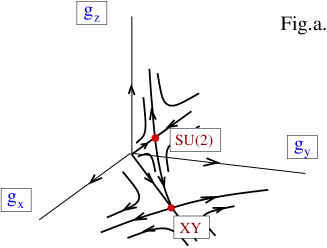
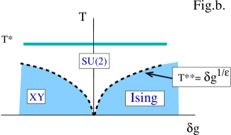
FIG. 1.: Fig. (a) Sketch of the renormalization flows in the purely bosonic model. We find one non-trivial SU(2)-invariant fixed point and three fixed points with XY symmetry. Both are unstable against breaking the SU(2) and XY symmetries, respectively. Fig. (b) Quantum phase transition in the purely bosonic model with XY symmetry as the anisotropy, $\delta g=g_{z}-g_{\perp}$ changes sign. The dashed lines indicate cross-over regions corresponding to $T^{**}$.

Even the behavior of the purely bosonic model is already very rich. In a realistic case, a number of cross-overs may occur between SU(2)-type, XY or Ising behaviors. In particular, for a system with XY-type symmetry a quantum phase transition occurs between the XY-type and Ising fixed points as $\delta g\equiv g_{z}-g_{x}=g_{z}-g_{y}$ changes sign (see Fig 1). In this case, the quantum phase transition is controlled by the SU(2) type fixed point below an energy scale $T^{*}$. For small $g_{\perp}=g_{x}=g_{y}\approx g_{z}\equiv g$ one can determine $T^{*}$ by integrating the scaling equations Eq. (9), and is approximately given by

$$T^{*}\sim\Lambda_{0}g^{1/\epsilon}.$$

As $T\to 0$ another cross-over occurs at an energy scale

$$T^{**}\sim(\delta g)^{y_{r}}T^{*}\;,$$

where $y_{r}=\epsilon/2+\epsilon^{2}/2+...$ is the scaling dimension of spin-anisotropy at the SU(2) fixed point. Between $T^{*}$ and $T^{**}$ the SU(2)-invariant Bosonic model describes the behavior of the impurity, while below $T^{**}$ the physical properties of the model are controlled by the Ising ($\delta g>0$) or the XY-type ($\delta g<0$) bosonic fixed points, respectively.

If $g_{x}\neq g_{y}$ then the behavior is even more complicated, and eventually two cross-overs may occur in series, corresponding to the $SU(2)\to XY$ and $XY\to Ising$ transitions. The cross-over regions are governed in this case by the SU(2) and XY-type fixed points, respectively.

Although anisotropy is relevant at both ${\cal O}(\epsilon)$ fixed points above, in many cases the SU(2)-invariant or XY-type fixed points can be also of physical interest: In the case of couprates, e.g.,[13] spin-orbit interaction is weak and therefore the anisotropy is presumably weak. In this case the SU(2)-symmetrical fixed point may appropriately describe the physics over a wide energy range of interest. On the other hand, in most magnetic heavy Fermion compounds spin-spin interactions are generically anisotropic,[19] and the physics is controlled by XY type or Ising fixed points.

2 The SU(2) symmetric Bose-Fermi Kondo Model

For the sake of clarity, we first discuss the renormalization group flows in the $SU(2)$ symmetric case with $g_{x}=g_{y}=g_{z}\equiv g$ and $\lambda_{x}=\lambda_{y}=\lambda_{z}\equiv\lambda$. The results we obtain to second order in $\epsilon$ are qualitatively the same as the leading order ones derived in Refs. [11, 12]. The flows are sketched in Fig. 2. Two stable quantum phases appear: (a) The Kondo state ($\lambda\to\infty$, $g=0$): This is the familiar Kondo state.[20] The local moment is completely screened by the Fermions and forms a Fermi liquid. It is thus fully decoupled from the bosonic field. At the Kondo fixed point both anisotropy and the bosonic field are irrelevant. (b) Purely bosonic SU(2) invariant fixed point ($g\approx\epsilon/2$, $\lambda=0$): This is the same fixed point as the one we discussed in the previous subsection. At this fixed point the coupling to the Fermions is irrelevant, however, breaking the spin anisotropy, as discussed earlier, is a relevant perturbation. It is though a stable fixed point if for some reason exact SU(2) symmetry is guaranteed, however, it is generally unstable in non-cubic systems with spin-orbit interaction. At this fixed point the impurity is only partially screened.[13]

These two phases are separated by an interesting quantum critical point: (c) The SU(2) symmetrical Bose-Fermi fixed point ($g\sim\lambda\sim\epsilon$). This fixed point governs the quantum phase transition between the bosonic and Fermionic SU(2) invariant phases in case of full SU(2) symmetry. However, similar to the SU(2) invariant Bose fixed point, anisotropy is relevant at this fixed point (in fact, it is the leading relevant operator, i.e., it is more relevant than the operator corresponding to the quantum phase transition.) Therefore, in general, it is not this fixed point that controls the quantum phase transition.

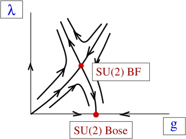
FIG. 2.: Renormalization group flows for the SU(2) symmetrical Bose-Fermi Kondo model. “BF” denotes the SU(2) symmetrical Bose-Fermi fixed point. Here the spin is partially screened and both the Fermi and Bose fields couple to it. At the Bose fixed point the fermionic degrees of freedom fully decouple from the spin.

3 The general case: Anisotropic BFKM

The general anisotropic Bose-Fermi Kondo model has all the fixed points discussed above. In addition, however, we find two new types of fixed points with XY and Ising symmetry: (a) The XY Bose-Fermi fixed point of the type $\lambda_{x}=\lambda_{y}\neq\lambda_{z}$ and $g_{x}=g_{y}\neq g_{z}=0$: Similar to the SU(2) Bose-Fermi fixed point, this fixed point separates the XY or Ising bosonic phases and the SU(2) invariant Kondo phase, and controls the quantum phase transition between them in case of XY symmetry.

Breaking the SU(2) symmetry is a relevant perturbation at the XY-Bose-Fermi fixed points too: It corresponds to an operator within the critical surface separating the bosonic and fermionic quantum phases. If we break the XY symmetry in this direction, the RG flows stay within the critical surface and end up in a new strong coupling fixed point: (b) The Ising Bose-Fermi fixed point with structure, $\lambda_{x}=\lambda_{y}\neq\lambda_{z}$ and $g_{x}=g_{y}=0\neq g_{z}$, with $g_{z},\lambda_{z}\sim 1$. This fixed point is outside the region of applicability of our perturbative RG. We believe, however, that this strong coupling fixed point is not a mere artifact of our approximations, and that this is the fixed point that should describe the phase transition in case of Ising symmetry.

The complicated structure of the flows and the connection between the various fixed points is summarized in Fig. 3.

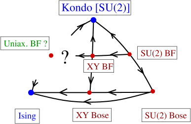
FIG. 3.: Summary of various fixed points and the possible flow directions.

B Physical quantities

Within the $\epsilon$-expansion, we can compute various physical quantities. The scaling properties of these are determined by the scaling dimensions and structure of the various relevant and irrelevant operators. Instead of enumerating all of these at each fixed point we rather list only the most important scaling dimensions in Table I.

At the ${\cal O}(\epsilon)$ fixed points we enumerated three scaling dimensions:
(a) The leading relevant operator: This is usually associated with breaking the symmetry of the fixed point.
(b) We also gave the scaling dimension of the most relevant operator respecting the symmetry of the fixed point. This operator at the Bose-Fermi fixed points corresponds to the quantum phase transition between the bosonic and fermionic fixed points with that symmetry.
(c) Finally, we also enumerated the scaling dimension of leading irrelevant operators, which determine the scaling properties of physical quantities at the quantum critical point (or the symmetry-stabilized XY or SU(2) Bose fixed points).

1 Susceptibility

Magnetic field is a relevant perturbation in all non-trivial ${\cal O}(\epsilon)$ fixed points. To study its effect we added the following term to the Hamiltonian:

$$H_{m}=-\sum_{\alpha=x,..,z}h_{\alpha}S_{\alpha}\;,$$ (10)

where $h_{\alpha}$ denote the components of a local magnetic field. As we shall prove later, the scaling equations of the dimensionless magnetic field, ${\tilde{h}}_{\alpha}\equiv h_{\alpha}/\Lambda$, are determined by the same beta-functions as those of the vertex $g_{\alpha}$:

$${d{\rm ln}{\tilde{h}}_{\alpha}\over dl}=1-{\epsilon\over 2}+{1\over 2g_{\alpha}}\beta^{(b)}_{\alpha}(\{\lambda_{\gamma}\},\{g_{\gamma}\})+{\cal O}({\tilde{h}})\;.$$ (11)

This remarkable result, which is very similar to the one obtained in Ref. [18] and follows from a Ward identity, has important consequences: By Eq. (7) it implies that at a fixed point with coupling $g_{\alpha}^{*}\neq 0$, the scaling dimension of the $\alpha$ component of the local magnetic field only depends on the anomalous dimension of the bosonic bath, and is exactly given by $y_{h,\alpha}=1-\epsilon/2$.

As explained in Ref. [21],e.g., the dimension $x_{\cal O}$ of a scaling operator ${\cal O}$ at a non-trivial fixed point is defined through the asymptotic behavior of its correlation function: $\langle{\cal O}({\bf r}){\cal O}({\bf 0})\rangle\sim 1/r^{2\;x_{\cal O}}$, where ${\bf r}$ denotes the coordinate variable. The dimension $x_{\cal O}$ is directly related to the scaling dimension $y_{H}$ of the dimensionless field $H$ that couples to the the scaling operator: Since in a $D$-dimensional theory the free energy has a dimension $D$, $y_{H}=D-x_{\cal O}$. In our case the impurity spin lives in an effective $D=0+1$-dimensional space, therefore this relation immediately relates the scaling dimension of the magnetic field $h$ to that of the impurity spin $S$ as $x_{S}=1-y_{h}$. As a consequence, the spin correlation function at the SU(2)-invariant Bose and Bose-Fermi fixed points decays at $T=0$ temperature as

$$\chi^{SU(2)}_{\alpha\beta}(\tau) = \langle TS_{\alpha}(\tau)S_{\beta}(0)\rangle=\delta_{\alpha\beta}\chi(\tau)\;,$$ (12)

$$\chi(\tau) = {1\over(T^{*}\tau)^{\epsilon}}$$ (13)

with $T^{*}$, a dynamically generated energy scale similar to the Kondo scale. This result has been derived earlier for the SU(2)-invariant bosonic fixed point in Ref. [[13]].

At the XY fixed points, however, the scaling properties of the magnetic field depend on its direction. To be specific, let us assume that the value of the couplings at the fixed point is $g_{x}^{*}=g_{y}^{*}\neq g_{z}^{*}=0$. In this case, spin correlations of the $x$ and $y$ spin components decay at $T=0$ as

$$\chi^{(XY)}_{\perp}(\tau)={1\over(T_{\perp}^{*}\tau)^{\epsilon}}\;,$$ (14)

while the decay of correlations in the $z$-direction is fixed point specific:

$$\chi^{(XY)}_{z}(\tau)={1\over(T_{z}^{*}\tau)^{\eta_{z}}}\;,$$ (15)

where, up to second order in $\epsilon$, $\eta_{z}$ is given by $\eta_{z}=2\epsilon+\epsilon^{2}$ and $\eta_{z}=2\epsilon+7\epsilon^{2}/4$ for the XY Bose and XY Bose-Fermi Kondo fixed points, respectively. Note that Eqs. (13) and (14) are valid to all orders in $\epsilon$, while the exponents $\eta_{z}$ can be computed only approximately.

The results above apply only at $T=0$ temperature. On can, however, obtain the finite temperature form of the correlation functions and their Fourier transforms assuming conformal invariance at these non-trivial fixed points.[22] For the imaginary part of the Fourier transform of the local spin-spin correlation functions, measurable through neutron scattering experiments, we obtain the following scaling form:

$$\chi^{{}^{\prime\prime}}_{\alpha}=\Bigl{[}{T^{*}\over T}\Bigr{]}^{1-\eta_{\alpha}}f(\eta_{\alpha},{\omega\over T})\;{\rm sgn}\omega\;,$$ (16)

where the scaling function $f(\eta,x)$ behaves as

$$f(\eta,x)\approx\left\{\begin{tabular}[]{lr}$C_{>}\;|x|^{\eta-1}$&\phantom{nn} $|\omega|\gg T$,\\ $C_{<}\;|x|$&\phantom{nn} $|\omega|\ll T$.\end{tabular}\right.$$ (17)

The function $f(\eta,x)$ can be expressed analytically from the exact expression Eq. (62).

2 Resistivity

Here we only discuss the impurity resistivity at the quantum critical points, i.e., we assume that all relevant variables and symmetry breaking terms have been tuned to zero or vanish for reasons of symmetry. In this case, the temperature dependence of the resistivity is determined by the scaling dimension $y_{i}<0$ of the leading irrelevant operator. We enumerated this latter for the various fixed points in Table I.

The simplest way to obtain the resistivity is to compute the impurity scattering rate. This turns out to be proportional to $\sum_{\alpha}\lambda^{2}_{\alpha}(T)$, where $\lambda_{\alpha}(T)$ is the effective coupling at energy scale $\omega\sim T$ that can be computed from the scaling equations. Since at the bosonic fixed point the effective couplings $\lambda_{\alpha}$ vanish as $\sim\lambda_{\alpha}(T)\sim T^{\Delta}$ with a power $\Delta=-y_{i}$ the resistivity there also vanishes as

$$R_{\rm imp}^{\rm Bose}(T)\sim A\;T^{2\Delta}\;,$$ (18)

and the impurity fully decouples from the electrons at $T=0$.

The situation at the SU(2) and XY Bose-Fermi fixed points is, on the other hand, different. There the couplings scale to a finite value, corresponding to a finite scattering rate, and the leading corrections to this scale as

$$R_{\rm imp}^{\rm BF}(T)\sim A+B\;T^{\Delta}\;,$$ (19)

similar to the multichannel Kondo model.

The above results only apply for the case of a dilute system of independent impurities. For the dense systems the interaction between individual impurities must be taken into account which leads in general to a different temperature dependence.

C Implications for a dynamical mean field theory of locally quantum critical phase transitions

It has been shown in a beautiful series of neutron scattering measurements by Schröder et al. that the quantum critical behavior in $\rm CeCu_{5-x}Au_{x}$ is entirely local within experimental accuracy. This material shows a quantum phase transition from a non-magnetic heavy Fermi liquid state to a metallic antiferromagnetic state under $\rm Au$ doping. The Fermi liquid energy scale below which the Ce spins are screened appears to go to zero as one approaches the quantum critical point from the metallic side, indicating that at the quantum critical point (QCP) spins remain asymptotically free at low temperature.[17] Schröder et al. also find that at the quantum critical point the dynamic susceptibility behaves with a good accuracy as

$$\chi^{-1}(\omega,T,{\bf q})\sim{\rm cst.}(\chi^{-1}({\bf q})+(T-i\omega)^{\alpha})$$ (20)

with an exponent $\alpha\approx 0.75$, where $\chi^{-1}({\bf q})$ is an approximately frequency and temperature independent function with minima at the ordering wave vectors.

Clearly, the quantum phase transition in $\rm CeCu_{5-x}Au_{x}$ is driven by the competition between two mechanisms with which the system can get rid of the residual entropy of the Ce impurity spins: The Kondo effect that screens magnetic impurities individually, and the magnetic ordering, which tends to align spins and thus destroys the Kondo effect.

Expression (20) is consistent with the presence of mean-field-like spatial correlations but simultaneous non-trivial local correlations in the time direction. Based on these observations,[17] Si et al. proposed a self-consistent version of the Bose-Fermi Kondo model[15] as a good candidate to describe the above quantum critical behavior within a dynamical mean field approach.[23]

1 SU(2) invariant theory

In their work, Si et al. assumed that the system is $SU(2)$ symmetrical in spin space, and therefore identified the QCP with the SU(2) invariant Bose-Fermi fixed point. In this theory, the exponent $\epsilon$ must be determined self-consistently, and it is fixed by the condition that the correlation functions $\langle TS_{\alpha}(\tau)S_{\alpha}(0)\rangle$ and $\langle T\phi_{\alpha}(\tau)\phi_{\alpha}(0)\rangle$ must decay asymptotically with the same exponent.

As we have discussed above, at the SU(2) invariant Bose-Fermi fixed point $\langle{\bf S}(\tau){\bf S}(0)\rangle\sim{1/\tau^{\epsilon}}$ as a consequence of a Ward identity. Similar to the case of spin glasses,[9, 18] this immediately determines the only possible exponent:

$$\epsilon_{\rm QCP}^{\rm SU(2)}\equiv 1\;.$$ (21)

This result has dramatic consequences: (a) It implies that - if a stable self-consistent solution of the extended dynamical mean field theory exists - then local spin correlations decay as $1/\tau$ at the quantum critical point and thus the the local susceptibility must diverge logarithmically as a function of frequency or temperature. This may be consistent with the mean field expression (20) only if the magnetic fluctuations are approximately two-dimensional.[15] In this case the exponent $\alpha$ would be non-universal and would depend on the specific properties of the model. (b) As a consequence, the scaling dimension of the local magnetic field (i.e. a field applied only to the impurity) would be exactly $y_{h}^{\rm SU(2)}=1/2$. This in turn immediately implies an $h^{2}/T$ scaling, which is clearly in disagreement with the experimental data, showing an almost perfect $h/T$ scaling. However, in the experiments one applies a global field, and we know cases where the the scaling dimension of the global field is different from that of the local field acting only on the impurity.[13, 24] It is therefore conceivable that the global field could result in an $h/T$ scaling.

All these considerations are only valid at the SU(2) invariant Bose-Fermi Kondo fixed point. However, magnetic interactions in $\rm CeCu_{5-x}Au_{x}$ and most heavy fermion materials are strongly spin-anisotropic, and we have shown that anisotropy is relevant at the $SU(2)$-invariant Bose-Fermi Kondo fixed point.

Thus if there is any locally critical quantum field theory that describes the QCP, it must be anisotropic. One of the candidates for the non-trivial fixed points is the new XY Bose-Fermi fixed point. At this fixed point, the coupling to the $z$-component of the spin is irrelevant and scales to 0. This is therefore, a good candidate to describe systems like $\rm YbRh_{2}Si_{2-x}Ge_{x}$,[17], where magnetic fluctuations are more of XY-type.

In $\rm CeCu_{5-x}Au_{x}$, however, the magnetic degrees of freedom are more Ising-like. The corresponding quantum phase transition can therefore possibly be described by the Ising Bose-Fermi fixed point of the local model with structure $g_{x}=g_{y}=0$, $g_{z}\sim 1$, and $\lambda_{z}\neq\lambda_{x}=\lambda_{y}$.

2 XY invariant theory

As we discussed earlier, at this fixed point correlations in the $xy$ and $z$ spin directions decay with different powers. This immediately implies that in a self-consistent theory one must also assume that the $xy$ and $z$ components of the field $\phi_{i}$ have also different anomalous dimensions, $\epsilon_{\perp}$ and $\epsilon_{z}$. It is straightforward to generalize our computations to this case. Similar to the $\epsilon_{\perp}=\epsilon_{z}$ case, the asymptotic behavior of the correlations of the $xy$ spin components is determined by a Ward identity, and is given by $\langle S_{x}(\tau)S_{x}(0)\rangle\sim\langle S_{y}(\tau)S_{y}(0)\rangle\sim 1/\tau^{\epsilon_{\perp}}$, which yields again the exact relations,

$$\epsilon_{\perp,\rm QCP}^{XY}\equiv 1\;,$$ (22)

$$y_{h\;\perp}^{\rm XY}=1/2\;.$$ (23)

and implies conclusions similar to the ones drawn for the SU(2)-invariant fixed point for spin correlations within the $xy$ plane.

The other exponent, $\eta_{z}$, is however, not determined by a Ward identity And therefore the condition $\eta_{z}(\epsilon_{z})=2-\epsilon_{z}$ yields a non- trivial exponent $\epsilon_{z}\neq 1$. In leading order we find that $\epsilon_{z}$ vanishes, and it next order it turns out to be negative, indicating that the leading terms probably originate from analytic corrections and scale as $\langle S_{z}(\tau)S_{z}(0)\rangle\sim 1/\tau^{2}$. These results are, however, only approximate, and not very reliable, since the $\epsilon$-expansion formulas are not applicable any more for $\epsilon_{\perp}=1$.

3 Ising theory

As we mentioned above, in $\rm CeCu_{5-x}Au_{x}$ the magnetic degrees of freedom are more Ising-like. The corresponding quantum phase transition is therefore most probably be described by the Ising Bose-Fermi fixed point ($g_{x}=g_{y}=0$, $g_{z}\neq 0$, and $\lambda_{z}\neq\lambda_{x}=\lambda_{y}$) within a dynamical mean field theory. This fixed point leads out of the region of applicability of our $\epsilon$ expansion. Nevertheless, from the Ward identity it still follows that

$$\epsilon_{z,\rm QCP}^{\rm UNI}\equiv 1\;,$$ (24)

$$y_{h,z}^{\rm UNI}=1/2\;,$$ (25)

while the other exponents $\epsilon_{\perp}<1$ and $\eta_{\perp}>1$ are now determined by the specific form of the beta functions.

It is important to emphasize, that the prediction that for this locally critical dynamical mean field model local spin correlations in different directions decay with different powers and in one direction the decay is $\sim 1/\tau$ while in some other Direction(s) it decays with a larger power, is rather robust, and it should be possible to test it by polarized neutron scattering.

II Basic definitions

A Spectral representations

All calculations presented here were carried out in Matsubara space using the spectral representation of the various propagators. Though it is not necessary for the calculations, we found it rather useful and intuitive to construct also microscopic free Hamiltonians and fields that give rise to the local propagators in Eqs. (4) and (5).

We constructed the bosonic field $\phi$ in terms of one-dimensional bosons, $b_{\alpha}(k)$ as

$$\phi^{\alpha}\equiv\int_{-\Lambda}^{\Lambda}dk\;|k|^{1-\epsilon\over 2}{1\over\sqrt{2}}(b_{\alpha}(k)+b^{\dagger}_{\alpha}(-k))\;.$$ (26)

Here $b_{\alpha}(k)$ destroys a boson with polarization $\alpha$ and momentum $k$, and $\Lambda$ is the high-energy cut-off. The $b_{\alpha}(k)$’s are normalized such that $[b_{\alpha}(k),b^{\dagger}_{\beta}(k^{\prime})]=2\pi\;\delta_{\alpha\beta}\;\delta(k-k^{\prime})$. Using a free bosonic Hamiltonian to generate their dynamics:

$$H^{(0)}_{\phi}\equiv\sum_{\alpha=1}^{3}\int_{-\Lambda}^{\Lambda}{dk\over 2\pi}\;|k|\;b^{\dagger}_{\alpha}(k)b_{\alpha}(k)\;,$$ (27)

it can be readily verified that Eqs. (26) and (27) lead to the propagator (5) with a constant $\Gamma(2-\epsilon)$. Note that $\phi$ is not the usual free bosonic field corresponding to Eq. (27) that would be defined through

$$\varphi^{\alpha}(x)\equiv\int_{-\Lambda}^{\Lambda}dk\;{e^{ikx}\over\sqrt{2\;|k|}}\;(b_{\alpha}(k)+b^{\dagger}_{\alpha}(-k))\;.$$ (28)

It is also a trivial matter to show that the bosonic Matsubara Green’s functions can be represented as:

$${\cal D}^{(0)}(i\omega_{n}) = \int_{-\Lambda}^{\Lambda}d\xi\;{\varrho(\xi)\over i\omega_{n}-\xi}\;,$$ (29)

$$\varrho(\xi) = {\rm sgn}(\xi)\;|\xi|^{1-\epsilon}\;,$$ (30)

with $\varrho(\xi)$ the spectral function of the Bose field $\phi$.

Similarly, to represent the fermionic propagator we can use free one-dimensional chiral fermions, described by the Hamiltonian

$$H^{(0)}_{\psi}=\sum_{\sigma=\pm}\int_{-\Lambda}^{\Lambda}{dk\over 2\pi}\;v_{F}k\;\psi^{\dagger}_{k,\sigma}\psi_{k,\sigma}\;,$$ (31)

with $v_{F}\equiv 1$ the Fermi velocity. The fermion field $\psi^{\dagger}_{k,\sigma}$ creates a fermion with momentum $k$, spin $\sigma$, and energy $k$, and is normalized as $\{\psi^{\dagger}_{k,\sigma},\psi_{k^{\prime},\sigma}\}=2\pi\;\delta(k-k^{\prime})$. Then the correlation function of the field

$$\psi_{\sigma}\equiv\int_{-\Lambda}^{\Lambda}{dk\over 2\pi}\;\psi_{k,\sigma}\;,$$ (32)

behaves exactly as Eq. (4), and its Fourier transform can be represented as

$${G}^{(0)}(i\omega_{n})=\int_{-\Lambda}^{\Lambda}{d\xi\over 2\pi}{1\;\over i\omega_{n}-\xi}\;.$$ (33)

B Pseudofermion technique

In order to treat the spin dynamics in a field theoretical framework we used Abrikosov’s pseudofermion technique.[25] In this approach one represents the spin operator as $S^{\alpha}\to\sum_{m,m^{\prime}}f^{\dagger}_{m}S^{\alpha}_{mm^{\prime}}f_{m^{\prime}}$, where $f_{m}$ is a pseudofermion annihilation operator corresponding to the $S^{z}=m$ spin component. In terms of these pseudofermions, the interaction terms can be treated using standard field theoretic methods. However, in order to obtain a faithful representation of the spin one has to project out unphysical states with $\sum_{m}f^{\dagger}_{m}f_{m}>1$. This is achieved by adding a term

$$H_{\rm ps}=\mu_{0}\sum_{m}f^{\dagger}_{m}f_{m}$$ (34)

to the Hamiltonian, taking the chemical potential $\mu_{0}\to\infty$, and keeping only the leading contributions in the end of the calculation.

The propagation of free pseudofermions is described by the Matsubara Green’s function

$${\cal G}_{mm^{\prime}}^{(0)}(i\omega_{n})\equiv-\langle Tf_{m}f^{\dagger}_{m^{\prime}}\rangle^{(0)}_{i\omega_{n}}={\delta_{mm^{\prime}}\;\over i\omega_{n}-\mu_{0}}\;.$$ (35)

III Renormalization Group

In order to analyze the behavior of the Bose-Fermi Kondo model at its non-trivial fixed points, we used field theoretical renormalization group methods, and applied expansion in the small parameter $\epsilon$.

A Spurious divergences and counterterms

Simple power counting shows that the pseudofermion self-energy contains ’spurious’ contributions that diverge as $\sim\Lambda$. These contributions only renormalize the chemical potential, $\mu_{0}\to\mu$, however, they lead to spurious divergences in higher order diagrams, and must therefore be removed.

To remove these divergences, we applied a counterterm procedure. In this approach we rewrite $H_{\rm ps}$ as

$$H_{\rm ps}=\mu\sum_{m}f^{\dagger}_{m}f_{m}+\delta\mu\sum_{m}f^{\dagger}_{m}f_{m}\;,$$ (36)

and formulate the perturbation theory in terms of $\mu$ rather than $\mu_{0}$:

$${\cal G}_{mm^{\prime}}^{(0)}(i\omega_{n})\to{\delta_{mm^{\prime}}\;\over i\omega_{n}-\mu}\;.$$ (37)

The term $\sim\delta\mu\sum_{m}f^{\dagger}_{m}f_{m}$ must be treated as a perturbation and it systematically cancels all spurious divergences in higher order diagrams. The coefficient $\delta\mu$ is determined self-consistently up to a given order of the perturbation theory by the requirement:

$$\Gamma^{(2)}\equiv{\cal G}^{-1}(i\omega_{n}=\mu)\equiv 0\;,$$

and is given in leading order by

$$\delta\mu={S(S+1)\over 3}{\Lambda\over 1-\epsilon}\sum_{\alpha}g_{\alpha}\;.$$

B Vertex functions

In order to compute the renormalization group equations, in addition to the inverse pseudofermion propagator $\Gamma^{(2)}$, we have to compute the ’three-point’ and ’four point’ vertex functions, $\Gamma_{\alpha}^{(3)}$ and $\Gamma_{\alpha}^{(4)}$ corresponding to the couplings $\gamma_{\alpha}$ and $\lambda_{\alpha}$ (see Fig. 4). This is straightforward (though somewhat tedious) within the pseudofermion technique.

As we shall see later, the fixed point couplings at the non-trivial fixed points turn out to be small, $\gamma_{\alpha}\sim{\cal O}(\sqrt{\epsilon})$ and $\lambda_{\alpha}\sim{\cal O}(\epsilon)$. This makes it possible to organize diagrams according to the powers of $\epsilon$ and perform a systematic expansion. The leading order diagrams are shown in Fig. 4.

Having removed all ’spurious divergences’ with the counterterm the diagrams contain only logarithmic infrared singularities $\sim{\rm ln}{\Lambda\over-\omega}$ in the $\epsilon\to 0$ limit, and can be expanded as a power of the logarithm. In leading order, the vertex functions are given by the following expressions:

$$\Gamma^{(2)} = \omega\Bigl{\{}1+{\rm ln}{\Lambda\over|\omega|}\;\;\bigl{[}{1\over 4}\sum_{\alpha}g_{\alpha}\bigr{]}\;+\dots\Bigr{\}}$$ (38)

$$\Gamma_{x}^{(3)} = \Lambda^{\epsilon/2}\gamma_{x}\Bigl{\{}1-{1\over 4}(g_{x}-g_{y}-g_{z})$$ (39)

$$+ {\rm ln}{\Lambda\over|\omega|}\;\;\bigl{[}{1\over 4}(g_{x}-g_{y}-g_{z})\bigr{]}\ +\dots\Bigr{\}}$$ (40)

$$\Gamma_{x}^{(4)} = \lambda_{x}\bigl{(}1-{1\over 4}(g_{x}-g_{y}-g_{z})\bigr{)}$$ (41)

$$+ {\rm ln}{\Lambda\over|\omega|}\;\;\Bigl{[}\lambda_{y}\lambda_{z}+{\lambda_{x}\over 4}(g_{x}-g_{y}-g_{z})\Bigr{]}+\dots$$ (42)

To perform the computation up to second order in $\epsilon$ 35 diagrams must be taken into account. Their list and the corresponding rather lengthy results are given in the Appendix.

C The renormalization group transformation

As mentioned above, once we removed all spurious divergences, the perturbation series contains only logarithmic divergences in the $\epsilon\to 0$ limit. These logarithmic divergences can be systematically summed up and treated using renormalization group methods.[26]

The chemical potential $\mu$ has, of course, no physical meaning. Therefore, once the unphysical contributions corresponding to multiple occupancy of the $f$-states have been eliminated,[27] we can transform it out by the transformation $i\omega_{n}\to\omega+\mu$. After this transformation, all quantities depend exclusively on $\Lambda$, the dimensionless couplings, and the ratio $\omega/\Lambda$.

To proceed further we define the pseudofermion $Z$-factor as

$${\partial\Gamma^{(2)}\over\partial\omega}\equiv Z^{-1}\bigl{[}\;{\omega/\Lambda},\;\{q_{i}\}\;\bigr{]}\;,$$ (43)

where $\{q_{i}\}$ ($i=1,..,6$) refers to the six dimensionless couplings of the theory, and $\Gamma^{(2)}$ denotes the inverse pseudofermion propagator.

Then the renormalizability of the theory implies that there exists a transformation $\Lambda\to\Lambda^{\prime}$, $q_{i}\to q_{i}^{\prime}$ such that the ’renormalized’ propagators and vertices remain invariant for all frequencies up to ${\cal O}(\omega/\Lambda)$ corrections:

$$\Gamma_{{\rm R}}^{(n)}\equiv Z\bigl{(}\;{\omega/\Lambda};q_{i}\bigr{)}\;\Gamma^{(n)}\bigl{(}\;\omega,\Lambda;q_{i}\bigr{)}=\mbox{fixed}\;,$$ (44)

where $\Gamma^{(2)}$ has been defined earlier, and $n=3$ and $n=4$ refer to the bosonic and fermionic vertex functions, respectively (see Fig. 4).

This invariance is expressed through the Callan-Symanzik equation:

$${d\over dl}{\rm ln}\Gamma_{\rm R}^{(n)}={\partial\over\partial l}{\rm ln}\Gamma_{\rm R}^{(n)}+\sum_{i}{dq_{i}\over dl}{\partial\over\partial q_{i}}{\rm ln}\Gamma_{\rm R}^{(n)}=0\;,$$ (45)

where we introduced the scaling parameter $l={\rm ln}(\Lambda_{0}/\Lambda$), with $\Lambda_{0}$ the bare value of the cut-off.

Substituting Eq. (44) into Eq. (45) we obtain the following differential equations:

$${\partial{\rm ln}\Gamma^{(n)}\over\partial l}+{\partial{\rm ln}Z\over\partial l}+\sum_{\alpha}{dq_{\alpha}\over dl}\left({\partial{\rm ln}\Gamma^{(n)}\over\partial q_{\alpha}}+{\partial{\rm ln}Z\over\partial q_{\alpha}}\right)=0\;.$$ (46)

To derive the scaling equations, we take the $\epsilon\to 0$ limit. Note that Eq. (46) is satisfied for all frequencies and temperatures provided that they are much smaller than the cut-off $\Lambda$. Therefore, expanding all vertex functions in powers of ${\rm ln}({\Lambda\over-\omega})$, the Callan-Symanzik equations can be obtained by just picking the constant terms and the terms proportional to ${\rm ln}({\Lambda\over-\omega})$. [Of course, in a renormalizable theory the same equations must be generated by comparing higher order terms in th expansion. Indeed, as a check we verified in leading order in $\epsilon$ that the same scaling equations are obtained from comparing the $\sim{\rm ln}({\Lambda\over-\omega})$ and $\sim{\rm ln}^{2}({\Lambda\over-\omega})$ terms too.] Plugging in the expressions of Eqs. (38-42) in the Eq. (46) we obtain the scaling equations Eq. (8) and Eq. (9). The second order ${\cal O}(\epsilon^{2})$ scaling equations are given in the Appendix.

FIG. 4.: Leading order corrections for the pseudofermion self-energy and vertex functions. Dashed lines stand for free pseudofermion propagators [Eq. (37)] wavy lines denote bosonic propagators [Eq. (29)] and continuous lines represent fermion propagators [Eq. (33)].

D Local magnetic field

1 Scaling equations

To investigate the effect of local magnetic field we have to add the term Eq. (10) to the Hamiltonian. As a consequence, ${\cal G}^{(0)}$ is modified to:

$${\cal G}^{(0)}={1\over i\omega-\mu+\sum_{\alpha}h_{\alpha}S^{\alpha}}\;,$$ (47)

and $\Sigma$ also becomes a matrix in spin space. Restricting the calculation to the case where $h$ represents the smallest energy scale in the problem, $|h|<\omega,T$, we can expand the renormalized inverse pseudofermion propagator as $\Gamma^{(2)}_{R}=Z\;\Gamma^{(2)}$ as

$$\Gamma^{(2)}_{R}\equiv Z\;[\Gamma^{(2)}_{0}+\sum_{\alpha}h_{\alpha}\Gamma^{(2)}_{1,\alpha}+{\cal O}(h^{2})]\;,$$ (48)

where $\Gamma^{(2)}_{0}$ and Z denote the inverse propagator and $Z$-factor in the absence of magnetic field, and $\Gamma^{(2)}_{1,\alpha}$ is also a matrix in spin space:

$$\Gamma^{(2)}_{1,\alpha}=-\Bigl{.}{\partial\Sigma\over\partial h_{\alpha}}\Bigr{|}_{h=0}\;.$$ (49)

From the invariance of $\Gamma^{(2)}_{R}$ it immediately follows that the magnetic field satisfies the following scaling equations:

$${d\over dl}{\rm ln}\left[Zh_{\alpha}\Gamma^{(2)}_{1,\alpha}\right]=0\;.$$ (50)

However, $\Sigma$ only depends on $h$ through the propagator ${\cal G}^{(0)}$. Therefore $\Gamma^{(2)}_{1,\alpha}$ is proportional to the functional derivative ${\delta\Sigma/\delta{\cal G}}$, and thus the bosonic vertex function by the Ward identity:

$$\Gamma^{(2)}_{1,\alpha}=-\Bigl{.}{\partial\Sigma\over\partial h_{\alpha}}=\Lambda^{-\epsilon/2}{1\over\gamma_{\alpha}}\Gamma_{\alpha}^{(3)}\;.$$ (51)

Another way to derive this equation is to notice that ${\cal G}^{(0)}$ can be expanded as

$${\cal G}^{(0)}={1\over i\omega-\mu}-\sum_{\alpha}h_{\alpha}{1\over i\omega-\mu}S^{\alpha}{1\over i\omega-\mu}+\dots\;\,$$ (52)

Differentiating $\Sigma$ with respect to $h_{\alpha}$ at $h=0$ thus amounts in diagrams where one of the pseudofermion lines has been replaced by an external vertex $\gamma_{\alpha}$ (see Fig. 5). It is easy to see that each vertex diagram is generated in this way exactly once and with the correct weight. Combining the Ward identity Eq. (51) with the invariance of the renormalized vertex function, ${d\over dl}{\rm ln}(Z\;\Gamma^{(3)})=0$, we immediately obtain that

$${d\over dl}{\rm ln}\Bigl{(}{h_{\alpha}\over\Lambda^{\epsilon/2}\gamma_{\alpha}}\Bigr{)}=0\;,$$ (53)

which, taking into account the definition of the $\beta$ function leads to the scaling equation:

$${1\over h_{\alpha}}{dh_{\alpha}\over dl}=-{\epsilon\over 2}+{1\over 2\;g_{\alpha}}\beta^{(b)}_{\alpha}(\lambda_{\alpha},g_{\alpha})\;,$$ (54)

or equivalently, Eq. (11) for the dimensionless magnetic field, $\tilde{h}=h/\Lambda$.

FIG. 5.: Diagrammatic representation of the Ward identity, Eq. (51).

E Susceptibility

There are two possibilities at a non-trivial fixed point with couplings $g_{\alpha}=g_{\alpha}^{*}$ and $\lambda_{\alpha}=\lambda_{\alpha}^{*}$:
(a) If $g_{\alpha}^{*}\neq 0$ then $\beta_{\alpha}^{(b)}(g_{\alpha}^{*},\lambda_{\alpha}^{*})=0$ and from Eq. (11) it follows that

$$\Bigl{.}{d{\tilde{h}}_{\alpha}\over dl}\Bigr{|}_{g^{*},\lambda^{*}}=(1-{\epsilon\over 2}){\tilde{h}}_{\alpha}\;.$$ (55)

This immediately implies the exact result for the $\alpha$ component of the spin correlation function at $T=0$:[21]

$$\langle TS^{\alpha}(\tau)S^{\alpha}(0)\rangle_{g^{*},\lambda^{*}}={1\over(T^{*}_{\alpha}\tau)^{\epsilon}}\;,\phantom{nnn}\mbox{if $g_{\alpha}^{*}\neq 0$},$$ (56)

with $T^{*}_{\alpha}$ a dynamically generated energy scale that is invariant under the scaling transformation, similar to the Kondo scale.[20]

On the other hand, if $g^{*}_{\alpha}=0$ then $\lim_{g^{*}_{\alpha}\to 0}\{\beta_{\alpha}^{(b)}(g_{\alpha}^{*},\lambda_{\alpha}^{*})/g^{*}_{\alpha}\}\neq 0$ takes some non-trivial value at the fixed point and no such universal relationship exists, and the spin-spin correlation function decays as

$$\langle TS^{\alpha}(\tau)S^{\alpha}(0)\rangle_{g^{*},\lambda^{*}}={1\over(T^{*}_{\alpha}\tau)^{\eta_{\alpha}}}\;,\phantom{nnn}\mbox{if $g_{\alpha}^{*}=0$},$$ (57)

with an exponent

$$\eta_{\alpha}=\epsilon-{\partial\beta_{\alpha}^{(b)}(g_{\alpha}^{*},\lambda_{\alpha}^{*})\over\partial g_{\alpha}^{*}}\;.$$ (58)

The spin correlation functions decay as a power law only at $T=0$ temperature. It is, however, easy to extend these results to finite temperature by assuming that there exists a boundary conformal field theory[22] that corresponds to the critical dynamics of the fixed point. In this boundary conformal field theory the impurity lives at the $x=0$ line of the complex plane, $z=\tau+ix$, and the theory is invariant under conformal mappings that map this boundary onto itself.

The finite temperature correlation functions can be obtained by mapping the complex plane on a strip of width $\beta=1/T$ using e.g. the function $w={1\over\pi T}{\rm artg}\;z$. Assuming that $S_{\alpha}$ transforms as a primary field of dimension $\eta_{\alpha}/2$

$$\langle S^{\alpha}(w_{1})S^{\alpha}(w_{2})\rangle_{T}=$$ (59)

$$\phantom{nnn}=\Bigl{(}{\partial z_{1}\over\partial w_{1}}\Bigr{)}^{\eta_{\alpha}/2}\Bigl{(}{\partial z_{2}\over\partial w_{2}}\Bigr{)}^{\eta_{\alpha}/2}\langle S^{\alpha}(z_{1})S^{\alpha}(z_{2})\rangle_{0}\;,$$ (60)

we obtain that at the critical point:

$$\chi_{\alpha}(\tau,T)=\Bigl{(}{\pi T\over T_{\alpha}^{*}{\rm sin}(\pi T\tau)}\Bigr{)}^{\eta_{\alpha}}\;.$$ (61)

Taking then the Fourier transform of Eq. (61) and continuing it analytically to the real axis one obtains an exact expression of the finite temperature susceptibility:[22]

$$\chi_{\alpha}(\omega)={T^{\epsilon}\over{T_{\alpha}^{*}}^{\epsilon}}{\pi^{\epsilon-1/2}\over T}{\Gamma({1\over 2}-{\eta_{\alpha}\over 2})\Gamma({\eta_{\alpha}\over 2}-{i\omega\over 2\pi T})\over\Gamma({\eta_{\alpha}\over 2})\Gamma({1\over 2}-{\eta_{\alpha}\over 2}-{i\omega\over 2\pi T})}\;.$$ (62)

The scaling form Eq. (16) readily follows from the asymptotic properties of the $\Gamma$ function.

IV Conclusions

In the present paper we analyzed the anisotropic Bose-Fermi Kondo problem using $\epsilon$-expansion methods. We found that in agreement with Ref. [12], spin anisotropy is relevant at the purely bosonic and Bose-Fermi fixed points.

We found two types of new bosonic fixed points: One one of them has XY symmetry, and is unstable against breaking the XY symmetry. This fixed point may be relevant for non-magnetic impurities in antiferromagnets at their quantum critical point with easy plain anisotropy, and it may also describe the coupling of the spins to the Goldstone modes in an ordered phase of an antiferromagnet [28]. The other fixed point has an Ising-like structure, and is stable. This fixed point could be relevant for non-magnetic impurities in an Ising antiferromagnet at the quantum critical point.

We identified furthermore two new Bose-Fermi quantum critical points in the impurity model with XY and Ising symmetries, respectively, which parallel the bosonic fixed points and separate the bosonic and fermionic quantum phases. We have shown that local spin correlations at these fixed points decay as $\langle TS_{x,y}(\tau)S_{x,y}(0)\rangle\sim 1/\tau^{\epsilon}$ and $\langle TS_{z}(\tau)S_{z}(0)\rangle\sim 1/\tau^{\epsilon}$ at the XY and Ising fixed points, respectively, as guaranteed by a Ward identity. Correlations in the other directions decay faster with non-universal exponents that we computed to second order in $\epsilon$. These fixed points may be relevant at the locally quantum critical points of $\rm YbRh_{2}Si_{2-x}Ge_{x}$ and $\rm CeCu_{5-x}Au_{x}$, respectively.[16, 29]

As discussed in detail in the Introduction, these results have very important implications for a possible dynamical mean field theory of the locally quantum critical behavior [15]:
(i) First of all, they imply that the real part of the local susceptibility diverges logarithmically at the quantum critical point in the easy axis/easy plain directions, $\chi_{\rm easy,local}^{{}^{\prime}}(\omega)\sim{\rm ln}(T^{*}/\omega)$, while the imaginary part is singular, $\chi_{\rm easy,local}^{{}^{\prime\prime}}(\omega)\sim{\rm sgn}(\omega)$. In the other directions, however, the local susceptibility should show a power-law behavior, $\chi_{\rm not-easy,local}^{{}^{\prime}}(\omega)\sim\omega^{\alpha}$, $\chi_{\rm not-easy,local}^{{}^{\prime\prime}}(\omega)\sim\omega^{\beta}$, and is likely to be dominated by analytic contributions with $\alpha=0$ and $\beta=1$. These predictions should be directly observable by polarized neutron scattering and NMR relaxation measurements.
(ii) A logarithmically divergent local susceptibility is consistent with the experimental scaling form, Eq. (20), only if the magnetic fluctuations are effectively two-dimensional. This quantum critical behavior can therefore be only approximate, and if it applies to the systems above, then a cross-over to some other type of quantum critical behavior should occur at lower temperatures.
(iii) Finally, the above results imply an $h^{2}/T$ scaling for the local magnetic field. Whether this is consistent with the experimentally observed $h/T$ scaling with the global field, is an open question that needs to be answered.

Note added: After completing this work we learned that a similar $\epsilon$ expansion has been carried out by L. Zhu and Q. Si with very similar results.[31]

V Appendix

In this appendix we give a few detailed expressions that may be important to reproduce or extend our results.

The easiest quantity to compute is the pseudofermion self-energy, whose diagrams are given in Fig 6 to ${\cal O}(\epsilon^{2})$, and correspond to the following expression:

$$\Gamma^{(2)}\approx\omega\Bigl{\{}1+\bigl{(}{1\over 4}\sum_{\alpha}(g_{\alpha}+\lambda_{\alpha}^{2})-{1\over 8}\sum_{\alpha\neq\beta}g_{\alpha}g_{\beta}+\bigr{)}\;{\rm ln}{\Lambda\over-\omega}\Bigr{\}}\;,$$ (63)

Note that the counterterm itself is also proportional to $\epsilon$ and is therefore important only in the ${\cal O}(\epsilon^{2})$ calculation.

FIG. 6.: Second order corrections in $\epsilon$ for the pseudofermion self-energy. The cross denotes the counterterm.

The expression of the bosonic vertex is somewhat lengthier:

$$\Gamma^{(3)}_{\alpha}=\Lambda^{\epsilon/2}\gamma_{\alpha}\Bigl{\{}F_{0}^{\alpha}(g_{\alpha},\lambda_{\alpha})+{\rm ln}{\Lambda\over-\omega}F_{1}^{\alpha}(g_{\alpha},\lambda_{\alpha})+\dots\Bigr{\}}\;,$$ (64)

where the coefficients $F_{0}$ and $F_{1}$ are given by

$$F_{0}^{x} = 1-{1\over 4}(g_{x}-g_{y}-g_{z})+{\cal O}(\epsilon^{2})\;,$$ (65)

$$F_{1}^{x} = {1-\epsilon\over 4}(g_{x}-g_{y}-g_{z})-{1\over 16}(g_{x}^{2}+g_{y}^{2}+g_{z}^{2})$$ (66)

$$+ {3\over 8}g_{x}(g_{z}+g_{y})-{7\over 8}g_{y}g_{z}$$ (67)

$$+ {1\over 8}(\lambda_{x}^{2}-\lambda_{y}^{2}-\lambda_{z}^{2})+{\cal O}(\epsilon^{2})\;.$$ (68)

The corresponding diagrams are depicted in Fig. 7.

FIG. 7.: Second order corrections in $\epsilon$ for the bosonic vertex function.

Finally, the vertex corrections to the usual Kondo interaction to this order are depicted in Fig. 8, and the corresponding expression reads:

$$\Gamma^{(4)}_{\alpha}=Q_{0}^{\alpha}(g_{\alpha},\lambda_{\alpha})+{\rm ln}{\Lambda\over-\omega}Q_{1}^{\alpha}(g_{\alpha},\lambda_{\alpha})+\dots\;,$$ (69)

where $Q_{0}$ and $Q_{1}$ are given by

$$Q_{0}^{x} = \lambda_{x}\bigl{(}1-{1\over 4}(g_{x}-g_{y}-g_{z})+{\cal O}(\epsilon^{2})\bigr{)}\;,$$ (70)

$$Q_{1}^{x} = \lambda_{y}\lambda_{z}\bigl{(}1+{1\over 4}(g_{y}+g_{z}-g_{x})\bigr{)}+\lambda_{x}\;F_{1}^{x}\;.$$ (71)

Here we only gave the $x$-component of the vertex functions, the others can be obtained by cyclic permutation.

FIG. 8.: Second order corrections in $\epsilon$ for the fermionic vertex function.

The scaling equations can then be simply obtained by substituting these expressions into Eq. (46) and are given by

$${d\lambda_{x}\over dl} = \lambda_{y}\lambda_{z}-{1\over 2}\lambda_{x}(g_{y}+g_{z})-{1\over 4}\lambda_{x}(\lambda_{y}^{2}+\lambda_{z}^{2})$$ (72)

$$+ {1\over 2}\lambda_{x}\bigl{(}g_{x}(g_{y}+g_{z})-g_{y}g_{z}\bigr{)}+{\cal O}(\epsilon^{4})\;,$$ (73)

$${dg_{x}\over dl} = g_{x}(\epsilon-g_{z}-g_{y})+g_{x}^{2}(g_{y}+g_{z})$$ (74)

$$- {1\over 2}g_{x}(\lambda_{y}^{2}+\lambda_{z}^{2})+{\cal O}(\epsilon^{4})\;.$$ (75)

[

Fixed point	$\{\lambda_{\alpha}\}$	$\{g_{\alpha}\}$	$\Delta=-y_{i}$	$y_{r}$	$y_{r}^{\rm symm}$	$R^{\rm imp}(T)$	Stability
Kondo $SU(2)$	$\lambda_{\alpha}=\lambda\to\infty$	$g_{\alpha}=0$	1	none	none	$C_{1}-C_{2}T^{2}$	STABLE
$SU(2)Bose$	$\lambda_{\alpha}=\lambda\neq 0$	$g_{\alpha}=0$	${\epsilon\over 2}+{\epsilon^{2}\over 8}$	${\epsilon\over 2}+{\epsilon^{2}\over 2}$	stable	$\sim T^{2\Delta}$	unstable
$SU(2)$ Bose-Fermi	$\lambda_{\alpha}=\lambda\neq 0$	$g_{\alpha}=g\neq 0$	${\epsilon}-{\epsilon^{2}\over 12}$	${\epsilon\over 2}+{7\epsilon^{2}\over 24}$	${\epsilon\over 2}+{\epsilon^{2}\over 6}$	$C_{1}+C_{2}T^{\Delta}$	unstable
XY Bose	$\lambda_{\alpha}=0$	$g_{x}=g_{y}\neq g_{z}=0$	${\epsilon/2}$	${\epsilon}+{\epsilon^{2}}$	stable	$T^{2\Delta}$	unstable
XY Bose-Fermi	$\lambda_{x}=\lambda_{y}\neq\lambda_{z}$	$g_{x}=g_{y}\neq g_{z}=0$	${\epsilon-{9\epsilon^{2}\over 8}}$	${\epsilon}+{3\epsilon^{2}\over 4}$	$0.618\epsilon+0.123\epsilon^{2}$	$C_{1}+C_{2}T^{\Delta}$	unstable
Uniax Bose-Fermi	$\lambda_{x}=\lambda_{y}\neq\lambda_{z}\sim 1$	$g_{x}=g_{y}=0,\;g_{z}\sim 1$	?	?	?	?	unstable
Uniax Bose	$\lambda_{\alpha}=0$	$g_{x}=g_{y}=0,\;g_{z}\to\infty$	?	none	stable	?	STABLE

TABLE I.: Stability and structure of the various fixed points in the absence of magnetic field: (a) $y_{i}$ is the dimension of the leading irrelevant operator. This exponent governs thermodynamics and scattering rates at the fixed point. (b) $y_{r}$ is the dimension of the leading relevant operator. This corresponds to breaking the symmetry of the fixed point. (c) $y_{r}^{\rm symm}$ is the scaling dimension of the leading relevant operator within the subspace of given symmetry. This governs the quantum phase transition between the Bosonic and Fermionic Kondo fixed points.

]

REFERENCES

- [1] I. Affleck, A.W.W. Ludwig, and B.A. Jones, Phys. Rev. B 52, 9528 (1995).
- [2] A. Georges and A.M. Sengupta, Phys. Rev. Lett. 74, 2808 (1995).
- [3] W. Hofstetter and H. Schoeller, Phys. Rev. Lett. 88, 016803/1 (2002); M. Vojta, R. Bulla, W. Hofstetter, Phys. Rev. B 65, 140405(R) (2002).
- [4] K. Kikoin and Y. Avishai, Phys. Rev. Lett. 86, 2090 (2001).
- [5] P. Schlottmann, Phys. Rev. Lett. 84, 1559 (2000).
- [6] A. Schiller, F.B. Anders, and D.L. Cox, Phys. Rev. Lett. 81, 3235 (1998).
- [7] M. Koga and D.L. Cox, Phys. Rev. Lett. 82, 2575 (1999).
- [8] W. G. van der Wiel, S. De Franceschi, J. M. Elzerman, S. Tarucha, L. P. Kouwenhoven, J. Motohisa, F. Nakajima, and T. Fukui, Phys. Rev. Lett. 88, 126803 (2002).
- [9] S. Sachdev and J. Ye, Phys. Rev. Lett. 70, 3339 (1993).
- [10] Q. Si and J. L. Smith, Phys. Rev. Lett. 77, 3391 (1996).
- [11] J. L. Smith and Q. Si, Europhys. Lett. 45, 228 (1999)
- [12] A.M. Sengupta, Phys. Rev. B 61, 4041 (2000).
- [13] M. Vojta, C. Buragohain, S. Sachdev, Phys. Rev. B 61, 15152 (2000); S. Sachdev, M. Troter, and M. Vojta, Phys. Rev. Lett. 86, 2617 (2001); S. Sachdev, Physica C 357-360, 78 (2001).
- [14] At a quantum critical point or in a d-wave superconductor the fermionic degrees of freedom may also have some anomalous dimension, but the discussion of this is out of the scope of the present paper.
- [15] Q. Si, S. Rabello, K. Ingersent, and L. Smith, Nature 413, 804 (2001); for details see Q. Si, S. Rabello, K. Ingersent, and L. Smith, cond-mat/0202414.
- [16] A. Schroder, G. Aeppli, R. Coldea, M. Adams, O. Stockert, H.v. Lohneysen, E. Bucher, R. Ramazashvili, and P. Coleman, Nature 407, 351 (2000).
- [17] P. Coleman, C. Pepin, Q. Si, and R. Ramazashvili, Journal of Physics (Condensed Matter) 13, 723 (2001).
- [18] A. Georges, O. Parcollet, and S. Sachdev, Phys. Rev. Lett. 87, 067202 (2001); A. Georges, O. Parcollet, and S. Sachdev, Physical Review B 63, 134406 (2001).
- [19] D.L. Cox and A. Zawadowski, Adv. Phys. 47, 599 (1998).
- [20] A.C. Hewson, The Kondo problem to heavy fermions (Cambridge University Press, 1993).
- [21] John Cardy, Scaling and renormalization in Statistical Physics (Cambridge University Press, 1997).
- [22] M.C. Aronson, M.B. Maple, P. De Sa, A.M. Tsvelik, R. Osborn, Europhys. Lett. 40, 245 (1997).
- [23] For a review on dynamical mean field theory see A. Georges, G. Kotliar, W. Krauth, and M.J. Rozenberg, Rev. Mod. Phys. 68, 13 (1996).
- [24] K. Ingersent and Q. Si, cond-mat/9810226.
- [25] A. A. Abrikosov, Physics 2, 5 (1965).
- [26] E. Brezin, J.C. Le Guillou, and J. Zinn-Justin, in Phase transitions and critical phenomena-Vol. 6, edited by C. Domb and M.S. Green (Page Bros. (Norwich) Ltd., 1996).
- [27] The fermions’ self energy in Fig. 6 is proportional to the thermal occupancy of the -states in the limit, . To obtain the physical self-energy one has to divide the one calculated with the pseudofermion technique by this quantity.
- [28] A. Castro-Neto et al. (private communication). In this work the purely bosonic and anisotropic problem is studied by a path integral approach yielding results very similar to ours.
- [29] O. Trovarelli, C. Geibel, S. Mederle, C. Langhammer, F.M. Grosche, P. Gegenwart, M. Lang, G. Sparn, and E. Steglich, Phys. Rev. Lett. 85, 626 (2000).
- [30] One can easily eliminate the -factor from Eq. (46) by subtracting the equation for from those of the vertex functions.
- [31] Q. Si (private communication).
- [32] We are especially grateful to Qimiao Si for discussions on the issue of scaling.