Dynamics of Competitive Evolution on a Smooth Landscape

Abstract

We study competitive DNA sequence evolution directed by in vitro protein binding. The steady-state dynamics of this process is well described by a shape-preserving pulse which decelerates and eventually reaches equilibrium. We explain this dynamical behavior within a continuum mean-field framework. Analytical results obtained on the motion of the pulse agree with simulations. Furthermore, finite population correction to the mean-field results are found to be insignificant.

Competitive evolution such as breeding has been practiced for ages. With recent advances in molecular biology, this method is widely used to develop novel proteins and DNA sequences for a variety of applications REF:Arnold2001 . The basic idea of competitive molecular evolution is straightforward: in each generation, a number of molecules with certain desired characteristics are selected from the population; they are then diversified (via point mutation and/or recombination REF:Stemmer1994 ) and amplified back to the original population size. The “speed” of evolution as well as the final equilibrium distribution depend on a variety of factors such as the mutation rate, selection strength, molecule length, and population size. A systematic quantitative understanding of these dependencies is lacking thus far. Such understanding is not only of theoretical interest, but also helpful in improving the efficiency of the breeding processes. In this study, we develop a theoretical model for the simplest type of competitive evolution involving only point mutations on a smooth landscape. We achieve an understanding of this model with concepts and techniques developed in the study of front propagation REF:Collet1990 .

To make the discussion concrete, we focus on the in vitro evolution of DNA sequences due to competitive binding to proteins. An example of such a system is the recent experiment of Dubertret et. al. REF:Dubertret2001 , where DNA sequences are selected competitively according to their relative affinities for the lac-repressor protein. In this experiment, selection is accomplished by coating a beaker with lac-repressor molecules followed by subsequent washing, so that only the strongly-bound sequences remain. Mutation and amplification are then accomplished by multiple stages of polymerase chain reaction REF:Lodish2000 . While the experiment of Ref. REF:Dubertret2001 easily accomplished the goal of finding the best binding sequence starting from a pool of random sequences in a few generations, the shortness of the binding sequence [$20$ base pairs (bp)] makes it difficult to explore the interesting dynamics of the competitive evolution process. In our study we consider the evolution process of Ref. REF:Dubertret2001 applied to much longer sequences so that that the steady state dynamics can be examined. An example of such a system might be the histone-octamer, which is known to bind DNA sequences of $147$ bp REF:Widom1999 .

We consider a pool of $N$ DNA sequences of length $L$. Each sequence ${\vec{S}}=(b_{1},b_{2},...,b_{L})$ of nucleotides $b_{i}$ is subject to independent single-nucleotide mutations at a rate $\nu_{0}\ll 1$ per nucleotide per generation. Selection is accomplished through protein-DNA binding. Let the binding energy of a sequence ${\vec{S}}$ to the protein be $E_{{\vec{S}}}$ and let the fraction of such sequences in the pool be $n_{{\vec{S}}}$. Assuming thermodynamic equilibrium for the binding process, the selection function is simply the binding probability, given by the Fermi function REF:VonHippel $P(E_{{\vec{S}}},\mu)=1/[1+\exp(E_{{\vec{S}}}-\mu)]$, where $mu$ is the chemical potential and all energies are expressed in units of $k_{\rm B}T$. Here $\mu$ serves as a (soft) selection threshold. and is determined by the fraction $\phi$ of DNA sequences that remain bound to the proteins after selection, i.e., $\sum_{{\vec{S}}}\,P(E_{{\vec{S}}},\mu)\,n_{{\vec{S}}}=\phi$. It can be controlled by either the number of available proteins or, as in the experiment REF:Dubertret2001 , by the washing strength. The fraction $\phi$ can be varied from $\phi\lesssim 1$ (weak competition) to $\phi\gtrsim 0$ (strong competition). We define the evolution process iteratively whereby in each round, $N$ daughter sequences are chosen from the existing pool according to $P(E_{{\vec{S}}},\mu)$, and then point mutation are introduced with rate $\nu_{0}$ to generate the new sequence pool.

Finally we need to specify the binding energy $E_{{\vec{S}}}$. We assume that each nucleotide taking part in the binding contributes independently, and adopt a “two-state” model REF:VonHippel which assigns an energy penalty $\epsilon$ (of the order of a few $k_{\rm B}T$’s) for each nucleotide which does not match the one the protein prefers. This form of binding energy has been shown to work reasonably well for specific systems fields and has been argued to hold for a wide class of regulatory proteins gmh , nonspecific . Given this energy model, a DNA sequence with $r$ mismatches has a binding probability $P(r,r_{0})=1\Big{/}\left[1+e^{\epsilon(r-r_{0})}\right]$, where $r_{0}\equiv\mu/\epsilon$ is the selection threshold in the “mismatch space” $r$. REF:Gerland2001 .

The above evolution model is easily implemented on a computer. We fix three of the model parameters at $N=5\times 10^{5}$, $L=170$ and $\nu_{0}=0.01$ from here on, and vary only the selection strength through the choice of the selection stringency $\phi$. A typical simulation result for strong selection ($\phi=0.1$) is shown as the space-time plot of the mismatch distribution $n(r,t)\equiv\sum_{{\vec{S}}}\,n_{{\vec{S}}}\,\delta(E_{{\vec{S}}}-r\epsilon)$ in Fig. 1. We see that the distribution quickly forms a shape-preserving pulse (see the inset of Fig. 1), which moves, decelerates, and eventually reaches equilibrium in the neighborhood of the optimal sequence (at $r=0$). Basically, the selection eliminates weak binders in the population to improve the average binding energy, hence the selection threshold $r_{0}$ is decreased in the next round, while the change of $r_{0}$ further selects sequences with better binding energies. Along with new variety generated by mutation, a propagating pulse results.

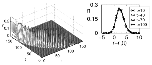
Figure 1: The space-time trajectory of the mismatch distribution $n(r,t)$ according to the competitive evolution model with $\phi=0.1$. The inset shows the distribution $n(r,t)$ at generations $t=10,40,70,100$, after the initial transient period and before the distribution reaches equilibrium at $r\approx 0$. These distributions overlap upon shift by their respective threshold $r_{0}(t)$, indicating the shape-invariance of the pulse.

We next investigate the dynamical behavior of the above evolution model analytically using a mean-field description. It will be convenient to describe the dynamics in the mismatch space $r$. Let us first consider the contribution from point mutation. For a sequence of length $L$, “alphabet size” ${\mathcal{A}}$ (${\mathcal{A}}=4$ for nucleotides) and $r$ mismatches, there are $L\cdot({\mathcal{A}}-1)$ ways to mutate to a new sequence via a single point mutation. Among them, there are $(L-r)({\mathcal{A}}-1)$ ways to increase $r$ by one, and $r$ ways to reduce $r$ by one. Hence, a standard master equation can be written to describe the mutational dynamics of the distribution $n(r,t)$ in the mean field limit $N\gg 1$ REF:Peliti1997 , REF:Drossel2001 , REF:Gerland2001 . The effect of selection/amplification process can be phenomenologically modeled by an additive term proportional to $\phi^{-1}P(r,r_{0})$ for weak selection. Further taking the continuum limit in $r$ (valid in the limit of large $L$ and smooth population distribution), we arrive at the following mean-field description for $n(r,t)$ REF:Gerland2001 :

$$\partial_{t}n=\partial_{r}\left[\partial_{r}(D(r)\,n)-v(r)n\right]+\,U[r;n]\cdot n(r,t)$$ (1)

$$U[r;n]=\left[\phi^{-1}P(r,r_{0}(t))-1\right]/\tau,$$ (2)

The first two terms on the right-hand side of (1) result from the (conservative) mutational processes, with

$$D(r)=\frac{\nu}{2}\left(1-\frac{{\mathcal{A}}-2}{{\mathcal{A}}-1}\frac{r}{L}\right),\quad v(r)={\nu}\left(1-\frac{{\mathcal{A}}}{{\mathcal{A}}-1}\frac{r}{L}\right)$$ (3)

being the “diffusion coefficient” and “drift velocity” respectively REF:Gerland2001 , $\nu\equiv\nu_{0}L$. The $r$-dependences of $v$ and $D$ reflect the different phase space volume for the different mismatches. For example, the form of $v(r)$ ensures that the the distribution approaches the maximum entropy point with $\overline{r}=\frac{{\mathcal{A}}-1}{{\mathcal{A}}}L$ mismatches by mutation alone. The third term in Eq. (1) represents the effect of the selection/amplification, controlled by the growth function $U$ defined in Eq. (2). (The factor $\tau\sim O(1)$ denotes generation time.) Competition is explicitly manifested in the $n$ dependence of the growth function $U$, via the threshold $r_{0}(t)$ which is determined from the condition $\phi=\int drP(r,r_{0}(t))n(r,t)$. In Eq. (2), an overall shift in $U$ by the constant $-1$ has been included to ensure that the population size $N$ is conserved after selection/amplification, in accordance with the evolution process. This shift produces the desired competitive effect that individuals which bind better than the threshold $r_{0}(t)$ are reproduced and those not meeting the threshold decay away. In the actual analysis, we will approximate the Fermi function $P(r,r_{0})$ by a step function $\Theta(r_{0}-r)$, which turns out not to affect the qualitative behavior.

We will see that the simplicity of the continuum mean-field equation provides an analytic understanding of generic features of the evolutionary dynamics, including the existence of the decelerating, shape-preserving population pulse; it also provides an analytical estimate of the smallness of the finite-$N$ correction. However that quantitative differences do exist between our simplified description and the breeding schemes employed in the simulations and experiments, due to the phenomenological nature of simplified description, and the continuum approximations used in both the mismatch space and time. (A quantitatively more accurate approach has recently been developed by Kloster and Tang REF:Kloster2 .)

We start with the simplest case of infinite sequence length (while keeping $\nu$ a finite constant), yielding constant coefficients $D(r)=D$ and $v=\nu$. Making the Ansatz in Eq. (1) that the distribution $n(r,t)=n[y(r,t)]$ where $y\equiv r-r_{0}(t)$ and $r_{0}(t)=-ct$ for some constant speed $c$, we obtain the ODE

$$Dn^{\prime\prime}(y)-[(c+\nu)n(y)]^{\prime}+u(y)n(y)=0,$$ (4)

where $u(y)\equiv\left({\phi}^{-1}\Theta(-y)-1\right)/\tau$. A physically allowed solution of Eq. (4) exists for every $c\geq c_{0}-\nu$, where

$$c_{0}\equiv\sqrt{4D({\phi}^{-1}-1)/\tau}.$$

In fact, the smallest possible speed $c_{\rm min}\equiv c_{0}-\nu$ is selected by the dynamics given a reasonably compact initial distribution. Here, velocity selection follows the familiar marginal stability mechanism REF:Collet1990 : The selected solution $n^{*}(y)$ (with the velocity $c_{\rm min}$) is the one that decays most sharply at the pulse front (i.e., the $r<r_{0}$ end) among all the allowed solutions. Thus, as the front of the distribution broadens from the initial condition, it first reaches the asymptotic decay of $n^{*}$. From then on, the distribution stops broadening and moves with the speed $c_{\rm min}$. Standard arguments show that this is equivalent to the condition that the front be marginally stable in the frame of reference moving with $c_{\rm min}$. Note that as $c_{0}\propto\sqrt{D}\propto\sqrt{\nu}$, $c_{\rm min}<0$ when the mutation rate $\nu$ is sufficiently large, indicating the worsening of the overall affinity of the sequences due to accumulation of deleterious mutations despite the presence of selection. These results apply also to the more general Fermi function, as it is only the asymptotic behavior of the growth term [i.e., $U(r\ll r_{0})$] that governs velocity selection.

In evolutionary dynamics, the population size $N$ often plays a very important role REF:Peliti1997 , REF:Drossel2001 . To see how $N$ enters, we note that the mean-field equation (1) has an inconsistency in that at the very front of the moving pulse, arbitrarily small $n$ gets the benefit of exponential amplification. But in reality, the number of individuals is discrete so that $n$ should always be greater than $1/N$. To deal with this problem, a cutoff procedure was proposed within the mean-field framework REF:Levine1996 , REF:Derrida1997 . Here we employ this procedure to estimate the effect of a finite population on the evolutionary velocity FNOTE:phasespace . Specifically, we modify the selection/amplification term $u(y)$ in Eq. (4) to $u(y)\Theta(n-N^{-1})$ (for $y<0$). A direct extension of the approach in Ref. REF:Derrida1997 leads to ${\delta c_{0}}/{c_{0}}\sim\frac{\pi^{2}}{2}/\ln^{2}N$ for the fractional change in $c_{0}$, which has the same scaling form as that for the Fisher equation REF:Derrida1997 . To test this result, we ran simulations (with a modified mutational scheme to achieve a constant drift) to measure the propagating speed of the pulse for different population sizes $N$. Our finding of $\delta c/c\approx 0.06$ between $N=5\times 10^{3}$ and $5\times 10^{8}$ is in line with the expectation and indicates that under typical experimental conditions, the fluctuation effect due to finite population is insignificant.

We next examine the more realistic situation of finite sequence length $L$. The important new effect is due to the $r$-dependence in the drift velocity $v(r)$ [see Eq. (3)], which, as the population approaches towards $r=0$, increasingly hinders its advance. This can already be appreciated if we assume a quasi steady-state dynamics and replace $\nu$ in the formula for $c_{\rm min}$ with $v(r)=\nu-\gamma r$ [where $\gamma\equiv\frac{4}{3}\nu_{0}$ according to (3)]: We find a stable stationary position, ${\overline{r}}^{\rm EQ}\approx(\nu-c_{0})/\gamma$ where $c_{\rm min}=0$. Here we identify this position naturally with the mean of the population ${\overline{r}}^{\rm EQ}\equiv\int rn^{\rm EQ}(r)dr$.

To proceed with a more rigorous analysis, we neglect the $r$ dependence in $D$ which has only a small quantitative effect. Also, we assume that the equilibrium position ${\overline{r}}^{\rm EQ}\gg 1$ so that the boundary condition at $r=0$ can be safely ignored.

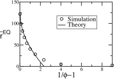
Figure 2: (a) Evolution of the mean mismatch ${\overline{r}}(t)$ for $\phi=0.5$. The equilibrium distribution is used as the initial condition to mitigate transient effects. The solid line is a single-exponential fit using the theoretical value of $\gamma=\frac{4}{3}\nu_{0}=.0133$. (b) Equilibrium positions as a function of selection pressure $\phi^{-1}-1$. The line is the theoretical estimate ${\overline{r}}^{\rm EQ}=(\nu-c_{0})/\gamma$, using a generation time $\tau=2.77$ (obtained by calibrating $c_{0}$ from theory with that from simulation).

Returning to the mean-field equation (1), we use the same moving-pulse Ansatz as before except that we no longer fix a linear time dependence to the threshold $r_{0}(t)$. This Ansatz produces a linear ODE for $r_{0}(t)$:

$$\gamma r_{0}(t)+{\dot{r}}_{0}(t)=\gamma r_{0}^{\rm EQ}$$ (5)

where $r_{0}^{\rm EQ}$ is the equilibrium threshold, so that a static distribution can be achieved in the moving frame. The population mean ${\overline{r}}$ follows exactly the same motion (in fact, ${\overline{r}}(t)\approx r_{0}(t)$ except when selection is very weak), i.e., a single exponential with time constant $\gamma$ (which depends only on the point mutation rate $\nu_{0}$). This is a generic result independent of the details of the fitness function, as long as a pulse solution exists for Eq. (1). The decay constant $\gamma$ obtained from simulation of the discrete model is in quantitative agreement with the expectation ($\frac{4}{3}\nu_{0}$) for weak selection ($1>\phi\gtrsim 0.25$); an example is shown in Fig. 2(a). In fact, the same qualitative result (i.e., the existence of a shape-preserving pulse) holds for strong selection as shown already in Fig. 1 where $\phi=0.1$.

The shape of the pulse, i.e. the equilibrium distribution $n^{\rm EQ}$, is governed by the same ODE as Eq. (4), except that the constant velocity $c$ is replaced by $-\gamma(y+r_{0}^{\rm EQ})$. The resulting equation again has a continuum of physically allowed solutions, each having a different shape and corresponding to a different equilibrium position $r_{0}^{\rm EQ}$ (hence different ${\overline{r}}^{\rm EQ}$). Here we have an interesting generalization of velocity selection to the selection instead from a continuum of decelerating pulses. Again, starting from a compact initial distribution, the dynamics selects the solution REF:Solutions whose front ($y<0$) decays most rapidly, (in this case a Gaussian falloff), whereas the other solutions have a power-law front.

The ${\overline{r}}^{\rm EQ}$ extracted from the selected solution agrees well with its heuristic approximation of $({\nu}-c_{0})/{\gamma}$ when ${\gamma}\ll 1$; see Fig. 2(b). The theory is quantitatively accurate FNOTE:Shape when the selection is not too strong (e.g., $\phi^{-1}<2.5$). For very strong selection, the equilibrium threshold position $r_{0}^{\rm EQ}$ approaches $r=0$ and the boundary condition there needs to be taken into account. When $c_{0}$ and $\gamma$ are expressed in terms of original parameters, ${\overline{r}}^{\rm EQ}=({\nu}-c_{0})/{\gamma}$ suggests that for a population with sequence length $L\gg 1$, the population pulse could stall at ${\overline{r}}^{\rm EQ}\gg 1$. In order for the population to reach the optimal at $r\approx 0$, we need to increase the selection strength (i.e., lowering $\phi$) or decrease the mutation rate so that $\phi^{-1}\gtrsim 1+\nu_{0}\tau L/2$, to overcome the bigger entropic barrier associated with longer sequences.

As there have been extensive studies of evolution on various landscapes in the context of population genetics REF:Burger2000 , REF:Peliti1997 , REF:Drossel2001 , it is worth comparing the dynamical behavior of competitive evolution with that of more common evolutionary models. The traditional study of evolution focuses on fixed fitness landscapes, where every genotype (e.g., sequence ${\vec{S}}$) has a predetermined absolute fitness value (i.e., the reproductive rate of the sequence ${\vec{S}}$). Competitive evolution is different in that it is subject to a dynamic fitness landscape. That is, the fitness is measured relative to a dynamic selection threshold and progress towards the best binding sequence occurs via competition among the currently existing genotypes — being better is all-important, not being best. This aspect of competitive evolution leads to qualitatively different dynamical behavior. For comparison, we can consider the simplest and most widely studied fixed landscape, i.e., the smooth “Mt. Fuji” landscape REF:Burger2000 , REF:Peliti1997 , REF:Drossel2001 , REF:Woodcock1996 , where each nucleotide contributes independently and additively to the fitness of the sequence, thus forming a landscape on which fitness rises steadily toward a single peak. For infinite sequence length, the mean-field theory fails in that it produces an unphysical, run-away solution REF:Levine1996 due to the unlimited growth rate of $n$ at the high fitness states  REF:Woodcock1996 , REF:Levine1996 , REF:Kessler1997andRidgeway1998 , and a finite population has a traveling speed that is essentially proportional to population size REF:Kessler1997andRidgeway1998 . For finite sequence length, the finite population dynamics is orders-of-magnitude slower in reaching equilibrium than the (now non-divergent) mean-field prediction REF:Kessler1997andRidgeway1998 . In contrast, finite population effects merely cause a small correction for the competitive evolutionary process.

To summarize, we investigated the dynamics of competitive evolution in the context of molecular evolution experiments. The major result concerns the existence and properties of a shape-invariant population pulse which propagates towards an eventual equilibrium configuration. Analytical results on the motion of the pulse obtained from the mean-field equation are in good agreement with simulations. Also, corrections due to finite population size are shown to be insignificant. An interesting aspect of our findings is the convergence of the evolution process to a solution far from optimal (i.e., ${\overline{r}}^{\rm EQ}\gg 1$), if the selection strength is not sufficiently strong or mutation rate not sufficiently low. In general, competitive evolution is rather different from the usual picture of climbing a fixed fitness landscape. This approach may be applicable more generally, e.g. to natural evolution in cases where competition for scarce resources is the primary driving force, as an organism only needs to be more efficient than its competitors to win the battle for evolutionary survival.

We thank M. Kloster for detail comments and discussions. We also acknowledge helpful discussions with D. Kessler, Q. Ouyang, L. Tang and J. Widom. This research is supported by the NSF through Grants DMR-0211308 and MCB-0083704.

References

- [1] E. T. Farinas, T. Bulter and F. H. Arnold, Curr. Opin. Biotechnol. 12, 545 (2001).
- [2] W. P. C. Stemmer, Nature 370, 389 (1994).
- [3] See, e.g., P. Collet and J. -P. Eckmann, Instabilities and Fronts in Extended Systems (Princeton University Press, Princeton, 1990).
- [4] B. Dubertret, S. Liu, Q. Ouyang and A. Libchaber, Phys. Rev. Lett. 86, 6022 (2001).
- [5] See, e.g., H. Lodish et. al., Molecular cell biology, th ed (W.H. Freeman & Co., New York, c2000).
- [6] A. Thastrom et al., J. Mol. Biol. 288, 213 (1999).
- [7] P. H. von Hippel and O. G. Berg, Proc. Natl. Acad. Sci. 83, 1608 (1986).
- [8] D.S. Fields, Y. He, A.Y. Al-Uzri and G.D. Stormo, J. Mol. Biol. 271, 178 (1997).
- [9] U. Gerland, J.D. Moroz and T. Hwa, Proc. Natl. Acad. Sci. 99, 12105 (2002).
- [10] To focus on the steady state dynamics, we have ignored “nonspecific” protein-DNA binding REF:VonHippel , gmh . This would affect the initial stage of evolution which plays a dominant role in the experiment of Ref. REF:Dubertret2001 .
- [11] U. Gerland and T. Hwa, J. Mol. Evol. 55, 386 (2002).
- [12] L. Peliti, cond-mat/.
- [13] B. Drossel, Adv. Phys. 50, 209 (2001).
- [14] M. Kloster and C. Tang, manuscript in preparation.
- [15] L. S. Tsimring, H. Levine and D. A. Kessler, Phys. Rev. Lett. 76, 4440 (1996).
- [16] E. Brunet and B. Derrida, Phys. Rev. E 56, 2597 (1997).
- [17] D. A. Kessler, H. Levine, D. Ridgway and L. Tsimring, J. Stats. Phys. 87, 519 (1997); ibid., 87, 519 (1997).
- [18] Strictly speaking, is the cutoff value in the sequence space () rather than the mismatch space (). As there is only selection in the mismatch space, the distribution forms a compact packet and undergoes random walk in the orthogonal direction. Hence, we expect the cutoff to be valid up to a constant even in mismatch space.
- [19] The selected solution can be expressed via the parabolic cylinder function , with [] for (), where [] and . is determined by matching conditions at .
- [20] Although the analytical solution gives a fair description of the motion of the pulse, it offers a pulse shape much broader than observed in simulation. A better description of the shape is presented in REF:Kloster2 .
- [21] See, e.g, R. Bürger, The Mathematical Theory of Selection, Recombination and Mutation (John Wiley & Sons, Chichester, UK, 2000).
- [22] G. Woodcock and P. G. Higgs, J. Theor. Biol. 179, 61 (1996).