Absence of self-averaging in the complex admittance for transport through disordered media

Abstract

Random walk models in one-dimensional disordered media with an oscillatory input current are investigated theoretically as generic models of the boundary perturbation experiment. It is shown that the complex admittance obtained in the experiment is not self-averaging when the jump rates $w_{i}$ are random variables with the power-law distribution $\rho(w_{i})\sim{w_{i}}^{\alpha-1}\ (0<\alpha\leq 1)$. More precisely, the frequency-dependence of the disorder-averaged admittance $\langle\chi\rangle$ disagrees with that of the admittance $\chi$ of any sample. It implies that the Cole-Cole plot of $\langle\chi\rangle$ shows a different shape from that of the Cole-Cole plots of $\chi$ of each sample. The condition for absence of self-averaging is investigated with a toy model in terms of the extended central limit theorem. Higher dimensional media are also investigated and it is shown that the complex admittance for two-dimensional or three-dimensional media is also non-self-averaging.

I INTRODUCTION

Disordered systems like amorphous semiconductors have a large number of remarkable properties inherent in their disorder, like the dispersive transport Scher91 . Hence, the disordered systems have wide areas of application like the photoreceptors of solar batteries and photocopiers Scharfe70 . So, they attract continuous research interests. In investigation of such remarkable properties, two kinds of statistics are to be considered. One is of course statistics of thermal fluctuation, which is considered in traditional statistical physics. The other is statistics of random structure of disordered systems. In order to treat this type of statistics, random structure is described with random variables and the probability distribution function of the random variables characterizes the substances.

It is usually assumed in studies of disordered systems that a sample used in experiments is sufficiently large. Hence, a measurement of any observable in such a system corresponds to an average over the ensemble of all realizations of the disorder. Quantities for which this assumption is valid are said to be self-averaging. The assumption means no sample dependence in the quantities. So, if the assumption is valid, reproducibility of experimental results for different samples is guaranteed. In addition, if the assumption is valid, in theoretical analyses only a disorder-averaged quantity is to be calculated since it should coincide with experimental results for any sample.

The expectation that the assumption of self-averaging is valid is based on the law of large numbers. The theorem says that the mean of independent random variables is equal to the expectation value with probability one. However, disordered systems such as amorphous semiconductors are strongly disordered, i.e., the expectation value of the random variables that describe structural disorder diverge. For example, the dispersive transport has been successfully explained by strongly disordered random variables Scher91 . In the theory of the dispersive transport, the transport is modeled by a random walk model on the disordered lattice where the dwell times of carriers at lattice sites are strongly disordered random variables.

The distribution of strongly disordered random variables is broad. Hence, properties of limited areas of samples like the maximal dwell time govern the macroscopic properties like the macroscopic mobility. One simple example is the finite contribution of the maximal term of a set of strong disordered random variables to the sum of the set (see Eq. (84) in appendix.). The properties of the limited areas with principal contribution fluctuate from one sample to another. Hence, the macroscopic properties of such materials may fluctuate. Thus, the assumption of self-averaging should be tested for its validity in strongly disordered systems. In fact, there are several reports on absence of self-averaging in transport phenomena in disordered media: Ref. 3 for mean square displacement, ref. 4 for the mean first passage time in the Sinai model.

In this paper, we study theoretically self-averaging properties of physical quantities obtained in a boundary perturbation experiment. The experimental technique was introduced recently to measure the optoelectrical properties of amorphous semiconductors Jongh96 . In this experimental method, an oscillatory perturbation with laser light is applied at one end of a sample and a response of the photocurrent from the other end is measured. We use as a generic model of the boundary perturbation experiment a random walk model in a one dimensional lattice with a boundary condition oscillating in time. The potential surface that carriers in the amorphous semiconductors feel is rugged due to structural disorder and it is called a rugged energy landscape. Consequently, the jump rates of the carriers are random variables and its probability distribution characterizes the disorder. It is known that the random jump rates obeys the power-law distribution with a negative exponent Pfister78 and it implies that the energy landscapes of the disordered media are extremely rugged.

It is shown that the complex admittance obtained in the experiment is not self-averaging when the jump rates $w_{i}$ are random variables distributed by the power-law distribution with the negative exponent. More precisely, the frequency-dependence of the disorder-averaged admittance $\langle\chi\rangle$ disagrees with that of the admittance $\chi$ of any sample. It implies that the Cole-Cole plot of $\langle\chi\rangle$ shows a different shape from that of the Cole-Cole plots of $\chi$ of each sample. The condition for absence of self-averaging is investigated with a toy version of the complex admittance. The complex admittance for higher dimensional media is investigated and shown to be non-self-averaging.

The rest of this paper is organized in the following way: In Sec. II, the random walk model used in the present study is explained. In terms of random walk, the complex admittance is related to a more physically relevant quantity to describe the transport in a disordered medium in Sec. III. In Sec. IV, absence of self-averaging for the complex admittance of one-dimensional media is shown. In Sec. V, absence of self-averaging is displayed in the Cole-Cole plot impressibly. In order to understand the condition for absence of self-averaging, a toy model is studied with the extended central limit theorem in Sec. VI. Absence of self-averaging for higher dimensional disordered media is shown in the similar way for the one-dimensional case in Sec. VII. Discussions and conclusions including consideration of possibilities that non-self-averaging properties are observed in real experiments are given in Sec. VIII. A part of this work has been reported in the brief note Kawasaki00 without consideration based on the probability distribution of the normalized mean first passage time, study of the toy model and the results for higher dimensional media.

II A generic model of the boundary perturbation experiment

Response of a system to an external field is a standard tool to be utilized in the study of condensed matter. Recently, the intensity modulated photocurrent spectroscopy Jongh96 has been introduced to investigate transport properties in amorphous semiconductors. In the experiment, the electrode is illuminated with a laser and the incident light intensity is harmonically modulated at frequency $\omega$. The light absorbed by an optical transition generates the photocurrent. The light intensity absorbed in the electrode consists of a background intensity and an oscillating component with small amplitude $\phi(\omega)$, which respectively gives rise to a steady state photocurrent and a harmonically varying photocurrent $\triangle i(\omega)$. Since the harmonically varying photocurrent $\triangle i(\omega)$ may show a phase shift with respect to the absorbed light flux $\phi(\omega)$, the optoelectrical admittance $\triangle i(\omega)/\phi(\omega)$ becomes a complex number.

Since in this experiment an oscillatory perturbation is applied at one end of a system and a response is measured, the experimental technique belongs to a generic method called the boundary perturbation method (BPM). In the presence of a periodically forced boundary condition on one end of the system, the output from the other end of the system is in proportion to the perturbation in the linear response regime and the proportionality constant is called the admittance. The frequency dependence of the admittance contains various information of the dynamics of the system. The BPM is expected to provide useful information on transport properties of disordered media.

We introduce as a generic model of the BPM a random walk model in one-dimensional disordered lattice segment of $N+1$ sites with an oscillatory input current (see Fig. 1).

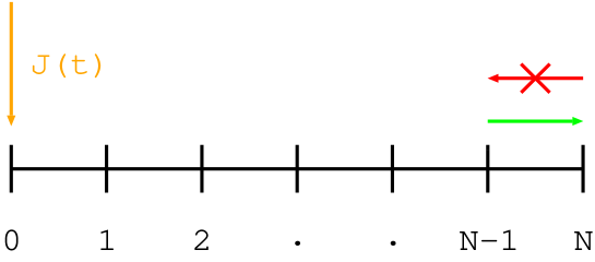
Figure 1: The structure of the one-dimensional lattice segment. The oscillatory current perturbation $J(t)$ is introduced at the site $0$. The site $N$ is assumed to be a sink.

The lattice sites are denoted by integers, $n=0,1,\ldots,N$. The dynamics of a random walking particle can be described by a master equation for the probability $P_{n}(t)$ that the particle is at the site $n$ at time $t\geq 0$. The master equation for the model is written as

$$\frac{dP_{n}(t)}{dt}=w_{n\ n-1}P_{n-1}(t)-(w_{n-1\ n}+w_{n+1\ n})P_{n}(t)+w_{n\ n+1}P_{n+1}(t),$$ (1)

where $w_{m\ n}$ denotes the random jump rate of a particle from the site $n$ to the site $m$. Here, we assume that the random walking particle jumps only to the nearest neighbor sites. The probability distribution of jump rates characterizes the disordered medium. We introduce a perturbation at the left end, so that the equation for $P_{0}(t)$ is given by

$$\frac{dP_{0}(t)}{dt}=-w_{1\ 0}P_{0}(t)+w_{0\ 1}P_{1}(t)+J(t).$$ (2)

$J(t)$ is the oscillatory current perturbation at the site $0$. The right end of the system is assumed to be a sink and the equation for $P_{N-1}$ is given by

$$\frac{dP_{N-1}(t)}{dt}=w_{N-1\ N-2}P_{N-2}(t)-(w_{N-2\ N-1}+w_{N\ N-1})P_{N-1}(t).$$ (3)

Since the current perturbation $J(t)$ oscillates in time around a positive average with the amplitude $\triangle J$, the response of the output current $w_{N\ N-1}P_{N-1}(t)$ oscillates around its stationary state with the amplitude $w_{N\ N-1}\triangle P_{N-1}$ at the same frequency with a phase-shift. The admittance is defined by the ratio of these two amplitudes

$$\chi_{N}(\omega)\equiv\frac{w_{N\ N-1}\triangle P_{N-1}}{\triangle J}.$$ (4)

The system of equations to determine the amplitudes $\triangle P_{n}$ of oscillation of the probabilities is derived from the master equation Eqs. (1), (2) and (3);

$$i\omega\triangle P_{n} = w_{n\ n-1}\triangle P_{n-1}-(w_{n-1\ n}+w_{n+1\ n})\triangle P_{n}$$

$$+w_{n\ n+1}\triangle P\ \ \mbox{for $n=2,3,\ldots,N-2$},$$

$$i\omega\triangle P_{0} = -w_{1\ 0}\triangle P_{0}+w_{0\ 1}\triangle P_{1}+\triangle J,$$

$$i\omega\triangle P_{N-1} = w_{N-1\ N-2}\triangle P_{N-2}-(w_{N-2\ N-1}+w_{N\ N-1})\triangle P_{N-1}.$$ (5)

III The complex admittance and the first passage time distribution

We show below that the admittance can be related to the first passage time distribution $F_{N\ 0}(t)$ (FPTD), which is the probability density that the particle which starts at the site $0$ at time $0$ arrives for the first time at the site $N$ at time $t$. Since the site $N$ is a sink, the FPTD is given by the output current from the site $N$ when there is no input current and the particle starts from the site $0$ at time $0$, i.e.

$$F_{N\ 0}(t)=w_{N\ N-1}P_{N-1}(t).$$ (6)

The Fourier-Laplace transform of the master equation for the case is written as

$$i\omega\tilde{P}_{n}(i\omega) = w_{n\ n-1}\tilde{P}_{n-1}(i\omega)-(w_{n-1\ n}+w_{n+1\ n})\tilde{P}_{n}(i\omega)$$

$$+w_{n\ n+1}\tilde{P}(i\omega)\ \ \mbox{for $n=2,3,\ldots,N-2$},$$

$$i\omega\tilde{P}_{0}(i\omega) = -w_{1\ 0}\tilde{P}(i\omega)_{0}+w_{0\ 1}\tilde{P}_{1}(i\omega)+1,$$

$$i\omega\tilde{P}_{N-1}(i\omega) = w_{N-1\ N-2}\tilde{P}_{N-2}(i\omega)-(w_{N-2\ N-1}+$$ (7)

$$w_{N\ N-1})\tilde{P}_{N-1}(i\omega).$$

This set of equations is identical to Eq. (5) divided by $\triangle J$. It means that $\triangle P_{n}/\triangle J=\tilde{P}_{n}(i\omega)$ and hence the Fourier-Laplace transform of the FPTD $\tilde{F}_{N\ 0}(s=i\omega)$ is identical to $w_{N\ N-1}\triangle P_{N-1}/\triangle J$. Thus, from Eqs. (4) and (6), we conclude that the admittance is equal to the Fourier-Laplace transform of the FPTD;

$$\chi_{N}(\omega)=\tilde{F}_{N\ 0}(i\omega).$$ (8)

We make the low-frequency expansion of the admittance to see the behavior near the static limit. Since the admittance is given by the Fourier-Laplace transform of the FPTD, the admittance at zero frequency equals to unity due to normalization of the FPTD;

$$\tilde{F}_{N\ 0}(0)=\int_{0}^{\infty}dtF_{N\ 0}(t)=1.$$ (9)

The mean first-passage time (MFPT) $\bar{t}_{N}$, which is the first moment of the FPTD, is given by $\bar{t}_{N}=i\ d\chi(\omega=0)/d\omega$. Thus, the low-frequency expansion of the admittance is given by

$$\chi_{N}(\omega)=1-i\ \bar{t}_{N}\ \omega+O(\omega^{2}).$$ (10)

The MFPT is given by Murthy89

$$\bar{t}_{N}=\sum^{N-1}_{k=0}\frac{1}{w_{k-1\ k}}+\sum^{N-2}_{k=0}\frac{1}{w_{k+1\ k}}\sum^{N-1}_{i=k+1}\prod^{i}_{j=k+1}\frac{w_{j-1\ j}}{w_{j+1\ j}}.$$ (11)

IV Absence of self-averaging for the complex admittance

Since we are interested in the complex admittance for amorphous semiconductors, we employ the power law probability distribution of the random jump rates Eq. (12), which is valid for amorphous semiconductors footnote1 :

$$\rho(w)=\left\{\begin{array}[]{ll}\alpha w^{\alpha-1}&\mbox{if $0<w<1$}\\ 0&\mbox{otherwise.}\end{array}\right.$$ (12)

There is possibility of the absence of self-averaging when disorder of the random dwell time at a site is strong as suggested in Sec. I. Since the dwell time is proportional to inverse of the jump rate, we are interested in the case where the first inverse moment of the random jump rate $\langle 1/w\rangle$ diverges, i.e. $0<\alpha\leq 1$. It is important to note that the inequality $0<\alpha<1$ holds for amorphous semiconductors Pfister78 .

IV.1 The probability distribution of the MFPT

In this subsection, we analyze the probability distribution of the MFPT Eq. (11). Since the MFPT gives the coefficient of the low frequency expansion of the admittance, the results of the analysis on the MFPT make it possible to determine whether the admittance is distributed with finite variance, i.e. non-self-averaging, or not. We show below that the complex admittance Eq. (10) is non-self-averaging when $0<\alpha<1$.

In order to analyze Eq. (11), we employ the random trap model general interest , where the jump rates $w_{ij}$ depends only on $j$. For the random barrier model, where the jump rates have the symmetry such that $w_{ij}=w_{ji}$, the quantitatively same results for self-averaging properties are obtained. We discuss below the probability distribution function of the normalized MFPT for the three cases of the value of $\alpha$. It is important to note that the three cases exhaust all possibilities of the value of $\alpha$. The choice of the normalization constants is suggested by the extended central limit theorem Feller66 . The theorem is summarized in appendix .1.

1. The case when $0<\alpha<1$ is considered. It is numerically shown that the probability distribution function of the normalized MFPT defined as $\bar{t}_{N}/N^{1/\alpha+1}$ converges to a distribution function with non-zero variance in the limit $N\rightarrow\infty$. Namely the normalized MFPT, $\lim_{N\rightarrow\infty}\bar{t}_{N}/N^{1/\alpha+1}$, is a random variable even for the infinitely long chain. In addition, the distribution function behaves asymptotically as $\rho(x)\sim x^{-\gamma}(1<\gamma<2)$ for large $x$. It is shown in Sec. VII.2 that $\gamma=\alpha+1$.

   

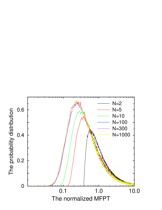
   Figure 2: The probability distribution function of the normalized MFPT $\bar{t}_{N}/N^{1/\alpha+1}$ for the random trap model where the probability distribution function of the random jump rates is power-law Eq. (12) with exponent $\alpha=1/2$. The distribution is computed from 500000 samples of disordered chains of the length $N=2,5,10,100,300,1000$. It is clearly seen that the probability distribution functions lie on a same curve when the length of lattice $N$ is sufficiently large.

   Figure 2 shows the probability distribution function of $\bar{t}_{N}/N^{1/\alpha+1}$ when $\alpha=1/2$ in Eq. (12). It is clearly seen that the probability distribution functions for sufficiently long chains lie on a same curve.

   

   Figure 3: The asymptotic behavior of the probability distribution function of the normalized MFPT computed from 5000000 samples. The solid line denotes the distribution function when $N=1000$ and $\alpha=1/2$ and the dashed line represents the function proportional to $x^{-1.5}$. One sees clearly that the distribution function behaves asymptotically as $\rho(x)\sim x^{-\gamma}(\gamma=1.5<2).$

   Figure 3 shows the tail of the probability distribution which appears in Fig. 2. It behaves asymptotically as $\rho(x)\sim x^{-\gamma}\ (\gamma=1.5<2)$.

2. When $\alpha=1$, it is numerically shown that the probability distribution function of the normalized MFPT defined as $\bar{t}_{N}/N^{2}-b_{N}/2$ converges to a distribution function with non-zero variance in the limit $N\rightarrow\infty$. Here, the centering constant $b_{N}$ is defined as

   $$b_{N}\equiv N\int^{\infty}_{1}dx\sin(x/N)x^{-2}.$$ (13)

   In appendix .2, we show that $b_{N}$ diverges as $N\rightarrow\infty$.

   

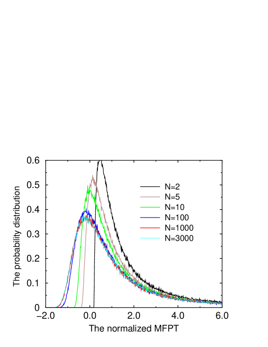
   Figure 4: The probability distribution function of the normalized MFPT $\bar{t}_{N}/N^{2}-b_{N}/2$ for the random trap model where the probability distribution function of the random jump rates is power-law Eq. (12) with exponent $\alpha=1$. The distribution is computed from 500000 samples of disordered chains of the length $N=2,5,10,100,300,1000,3000$. It is clearly seen that the probability distribution functions lie on a same curve when the length of lattice $N$ is sufficiently large.

   Figure. 4 shows the probability distribution function of the normalized MFPT when $\alpha=1$. It is clearly seen that the probability distribution functions lie on a same curve when the length of lattice $N$ is sufficiently large.

3. When $1<\alpha$, it is also shown numerically that the probability distribution function of the normalized MFPT defined as $\bar{t}_{N}/N^{2}$ converges to the Dirac delta function with the support at $\langle 1/w\rangle/2$. Figure 5 shows the probability distribution function of $\bar{t}_{N}/N^{2}$ when $\alpha=1.5$. One sees that the probability distribution concentrates on the point $\langle 1/w\rangle/2=1.5$ when the length $N$ is large.

   

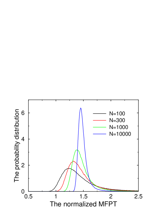
   Figure 5: The probability distribution function of the normalized MFPT $\bar{t}_{N}/N^{2}$ when $\alpha=1.5$. It is computed from 500000 samples of disordered chains of length $N=100,300,1000,10000$. It is seen clearly that the probability distribution concentrates on the point $\langle 1/w\rangle/2=1.5$ when the length of lattice $N$ is sufficiently large.

IV.2 Absence of self-averaging in the low frequency behavior of the complex admittance

By using the results for the probability distribution of the normalized MFPT, we discuss below frequency dependence of the complex admittance Eq. (10) for the three cases of the value of $\alpha$: $0<\alpha<1$, $\alpha=1$ and $1<\alpha$.

1. When $0<\alpha<1$, it is shown that the complex admittance is non-self-averaging. In order to see frequency dependence of the admittance, the long chain limit ($N\rightarrow\infty$) should be taken with keeping $\bar{t}_{N}\omega$ finite. Otherwise, the admittance becomes a trivial constant $0$ or $1$. Since it was shown that the normalized MFPT $\bar{t}_{N}/N^{1/\alpha+1}$ is finite with probability one, the long chain limit should be taken with fixing $\omega N^{1/\alpha+1}$ finite. Thus, from Eq. (10), the admittance for the infinitely long chain is given by

   $$\lim_{{N\rightarrow\infty}\atop{\;\tilde{\omega}=\omega N^{1/\alpha+1}}}\chi_{N}(\omega)=1-i\ \tilde{t}\ \tilde{\omega}+\ldots$$ (14)

   where $\tilde{t}$ is the normalized MFPT defined as $\tilde{t}\equiv\lim_{N\rightarrow\infty}\bar{t}_{N}/N^{1/\alpha+1}$ and $\lim_{{N\rightarrow\infty}\atop{\;\tilde{\omega}=\omega N^{1/\alpha+1}}}$ means the long chain limit with fixing $\omega N^{1/\alpha+1}$ at the finite value $\tilde{\omega}$. Equation (14) indicates that the admittance for the infinitely long chain is a function of the normalized MFPT $\tilde{t}$ and the scaled frequency $\tilde{\omega}$. From our result for the probability distribution of the normalized MFPT when $0<\alpha<1$, $\tilde{t}$ is a random variable. Thus, the admittance is also a random variable and hence the admittance is non-self-averaging.

2. When $\alpha=1$, it is shown below that the admittance is self-averaging in the low frequency range. By introducing the normalized MFPT $\tilde{t}_{N}$ defined as

   $$\tilde{t}_{N}\equiv\frac{\bar{t}_{N}}{N^{2}}-\frac{b_{N}}{2},$$ (15)

   $\bar{t}_{N}\omega$ is rewritten as

   $$\bar{t}_{N}\omega=N^{2}b_{N}\omega(\frac{2}{b_{N}}\tilde{t}_{N}+1)/2.$$ (16)

   It was shown in Fig. 4 that the normalized MFPT $\tilde{t}_{N}$ is finite with probability one. Thus, in order to see frequency dependence, the long chain limit should be taken with keeping the scaled frequency $\tilde{\omega}\equiv N^{2}b_{N}\omega/2$ finite. Since $b_{N}$ diverges as $N\rightarrow\infty$, the complex admittance for the infinitely long chain is given by

   $$\lim_{{N\rightarrow\infty}\atop{\;\tilde{\omega}=N^{2}b_{N}\omega/2}}\chi_{N}(\omega) = \lim_{{N\rightarrow\infty}\atop{\;\tilde{\omega}=N^{2}b_{N}\omega/2}}1-iN^{2}b_{N}\omega/2(\frac{2}{b_{N}}\tilde{t}_{N}+1)+\ldots$$ (17)

   $$= 1-i\tilde{\omega}+\ldots$$

   Since Eq. (17) has no sample-dependence, the complex admittance is self-averaging in the low frequency region.

3. When $1<\alpha$, it is shown below that the complex admittance is self-averaging. In this case, it was shown that the scaled MFPT $\bar{t}_{N}/N^{2}$ is equal to $\langle 1/w\rangle/2$ in the limit $N\rightarrow\infty$. Thus, the admittance for the infinitely long chain is given by

   $$\lim_{{N\rightarrow\infty}\atop{\;\tilde{\omega}=\omega N^{2}}}\chi_{N}(\omega)=1-\frac{1}{2}\left\langle\frac{1}{w}\right\rangle\tilde{\omega}+\ldots$$ (18)

   It means that the complex admittance is self-averaging.

From Eq. (14), the low-frequency expansion of the disorder-averaged admittance is given by

$$\langle\lim_{{N\rightarrow\infty}\atop{\;\tilde{\omega}=\omega N^{\beta}}}\chi_{N}(\omega)\rangle=1-i\ \langle\tilde{t}\rangle\ \tilde{\omega}+\ldots$$ (19)

When $0<\alpha<1$, the distribution function of the normalized MFPT $\tilde{t}$ behaves asymptotically as $\rho(x)\sim x^{-\gamma}$. It is shown later in Sec. VII.2 that $\gamma=\alpha+1$ and it means that $1<\gamma<2$. Hence, the expectation value $\langle\tilde{t}\rangle$ of the normalized MFPT diverges. Since it implies that the coefficient of the first order of low $\tilde{\omega}$ expansion diverges, the disorder-averaged admittance is a non-analytic function of $i\tilde{\omega}$ which must behave as

$$\langle\lim_{{N\rightarrow\infty}\atop{\;\tilde{\omega}=\omega N^{\beta}}}\chi_{N}(\omega)\rangle-1\sim(i\tilde{\omega})^{\mu}$$ (20)

where $0<\mu<1$.

In order to test the foregoing observation, we numerically solved Eq. (5) for one-dimensional chain of $20$ sites. The jump rate $w_{i\ j}$ depends only on $j$ (the random trap model) and the jump rates are generated from the power-law distribution Eq. (12). Figure 6 shows the low-frequency behavior of the real part and the imaginary part of the admittances when $\alpha=1/2$.

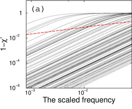
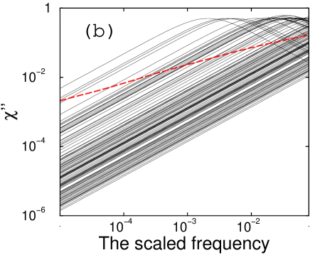
Figure 6: The frequency dependence of the real part (a) and the imaginary part (b) of the complex admittances when the exponent of the probability distribution of jump rates is $\alpha=1/2$ and the length of a chain is $N=20$. Solid lines represent the admittances for each of 100 samples. The dashed line represents the admittance averaged over 5000 samples. Though the admittance of each sample is proportional to the scaled frequency $\tilde{\omega}$, the averaged admittance is proportional to $\sqrt{\tilde{\omega}}$ ($\mu\simeq 1/2$).

One clearly sees that the low-frequency behavior of the disorder-averaged admittance is completely different from the admittance for any of the samples. On the other hand, figures 7 and 8 show the low-frequency behavior for $\alpha=1.0$ and for $\alpha=1.5$.

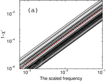
Figure 7: The frequency dependence of the real part (a) and the imaginary part (b) of the complex admittances when $\alpha=1.0$ and the length of a chain is $20$. Solid lines represent the admittances for each of 100 samples. The dashed line represents the admittance averaged over 5000 samples. Both the admittance of each sample and the averaged admittance are proportional to the scaled frequency $\tilde{\omega}$.

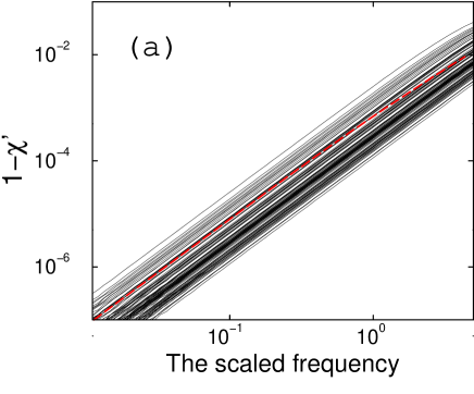
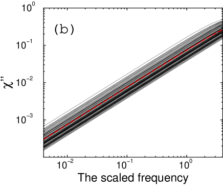
Figure 8: The frequency dependence of the real part (a) and the imaginary part (b) of the complex admittances when $\alpha=1.5$ and the length of a chain is $20$. Solid lines represent the admittances for each of 100 samples. The dashed line represents the admittance averaged over 5000 samples. Both the admittance of each sample and the averaged admittance are proportional to the scaled frequency $\tilde{\omega}$.

One clearly sees that the admittances for individual samples and their disorder-averaged admittance are both proportional to $\tilde{\omega}$. Although sample-dependence is observed, the sample-dependence is considered as the finite-size effect or effects from the terms of $O(\omega^{2})$.

V Non-self-averaging in the Cole-Cole plot

In the literature of experiments of the BPM Jongh96 , the Cole-Cole plot of the admittance is employed for the analysis of experimental results. It is a parametric plot of the imaginary part of the admittance against the real part.

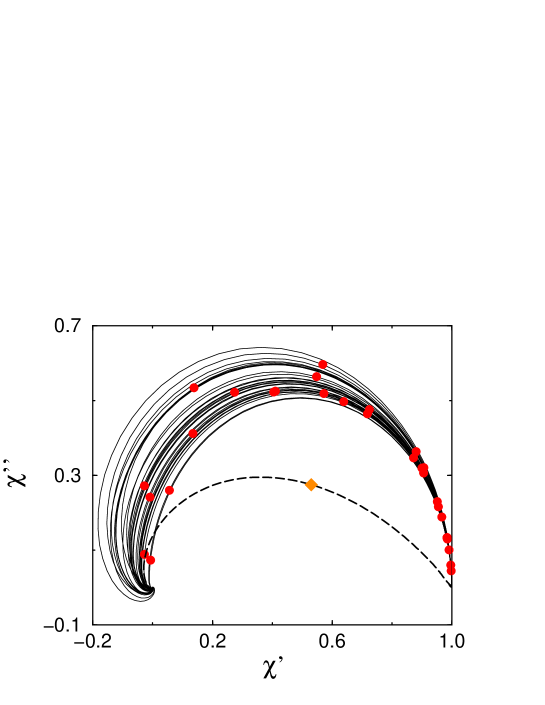
Figure 9: The Cole-Cole plots of the admittances when the exponent of the probability distribution of jump rates is $\alpha=1/2$ and $N=100$. Solid lines represent the admittances for each of 30 samples. The dashed line represents the admittance averaged over 5000 samples. The red solid circles represent the admittance of each sample at $\tilde{\omega}=0.5$. Although the red solid circles scatter outside the Debye semi-circle, the yellow diamond which denotes the averaged admittance at $\tilde{\omega}=0.5$ is inside of the Debye semi-circle.

Figure 9 shows the Cole-Cole plot of $\chi$ and $\langle\chi\rangle$ obtained by solving Eq. (5) when $\alpha=1/2$ in Eq. (12). One sees that the shape of the Cole-Cole plot of the disorder-averaged admittance is completely different from the shape of the Cole-Cole plot for each of samples. The boundary of the region where the Cole-Cole plot of the admittance of each sample scatters is the Debye semi-circle, whose center is at $(1/2,0)$ and the radius is $1/2$. In Fig. 9, solid circles denote the values of the admittance at a given frequency and a diamond is the average over these values. Since the admittance of each of samples at the same frequency (a solid circle) scatters around the Debye semi-circle, the admittance averaged at the same frequency (the diamond) comes inside the Debye semi-circle.

In order to analyze this non-self-averaging property of the admittance in the Cole-Cole plot, we prove rigorously that the Cole-Cole plots of each samples must lie outside the Debye semi-circle. We first note that the inverse of the admittance satisfies the following recursive relation:

$$\chi_{n}^{-1}(\omega)=\left(\frac{i\omega}{w_{n+1\ n}}+1+\frac{w_{n-1\ n}}{w_{n+1\ n}}\right)\chi^{-1}_{n-1}(\omega)-\frac{w_{n-1\ n}}{w_{n+1\ n}}\chi^{-1}_{n-2}(\omega),$$ (21)

where $\chi_{n}^{-1}(\omega)$ is the inverse of the admittance for a chain of length $n$. The recursive Eq. (21) is derived from the following two equations for the FPTD obtained from its definition: $\tilde{F}_{i+1\ i}(s)=\tilde{\psi}_{i+1\ i}(s)+\tilde{\psi}_{i-1\ i}(s)\tilde{F}_{i+1\ i-1}(s)$ and $\tilde{F}_{i+1\ i-1}(s)=\tilde{F}_{i+1\ i}(s)\tilde{F}_{i\ i-1}(s)$, where $\tilde{F}_{i\ j}(s)$ denotes the Laplace transform of the FPTD from site $j$ to site $i$ and $\tilde{\psi}_{i\ j}(s)$ denotes the Laplace transform of the waiting time distribution for the jump from site $j$ to site $i$. The recursive relation proves inductively that the inverse of the admittance obeys the following four inequalities in the frequency region $[0,\omega_{n}]$, where $\omega_{n}$ is the positive smallest zero of the real part of $\chi_{n}^{-1}$ and is equal to the positive smallest zero of ${\chi_{n}}^{\prime}$:

$$\left\{\begin{array}[]{l}{\chi_{n}^{-1}}^{\prime\prime}>0\\ {\chi_{n-1}^{-1}}^{\prime}>0\\ {\chi_{n}^{-1}}^{\prime\prime}>{\chi_{n-1}^{-1}}^{\prime\prime}\\ {\chi_{n}^{-1}}^{\prime}<{\chi_{n-1}^{-1}}^{\prime}.\end{array}\right.$$ (22)

Since the second inequality shows $\omega_{n}\leq\omega_{n-1}$, the fourth inequality implies ${\chi_{n}^{-1}}^{\prime}<{\chi_{n-1}^{-1}}^{\prime}<\cdots<{\chi_{1}^{-1}}^{\prime}=1$ in the region $[0,\omega_{n}]$. Since ${\chi_{n}^{-1}}^{\prime}={\chi_{n}}^{\prime}/({{\chi_{n}}^{\prime}}^{2}+{{\chi_{n}}^{\prime\prime}}^{2})$, the inequality ${\chi_{n}^{-1}}^{\prime}<1$ means $({\chi_{n}}^{\prime}-1/2)^{2}+{{\chi_{n}}^{\prime\prime}}^{2}>(1/2)^{2}$. Thus, the Cole-Cole plot of the admittance of each sample can exist only outside the Debye semi-circle when the frequency is smaller than the positive smallest zero of ${\chi_{n}}^{\prime}$.

On the other hand, we can show in the following way that the Cole-Cole plot of the averaged admittance is located inside the Debye semi-circle when $0<\alpha<1$. We consider the angle $\theta$ between the tangent of the Cole-Cole plot at (1, 0) and the horizontal axis. From Eq. (20), $\theta=\mu\pi/2$, which is less than $\pi/2$ since $\mu<1$, is obtained. However the angle $\theta$ for the Debye semi-circle is equal to $\pi/2$. It means that the Cole-Cole plot of the averaged admittance exists inside the Debye semi-circle when $0<\alpha<1$. Since the Cole-Cole plot of the admittance of any sample exists outside the Debye semi-circle, the Cole-Cole plot clearly shows non-self-averaging property of the admittance.

When $\alpha\geq 1$, the angle $\theta$ of the Cole-Cole plot of the averaged admittance is $\pi/2$ and is equal to that of the Cole-Cole plot of each of samples as seen in Figs. 10 and 11.

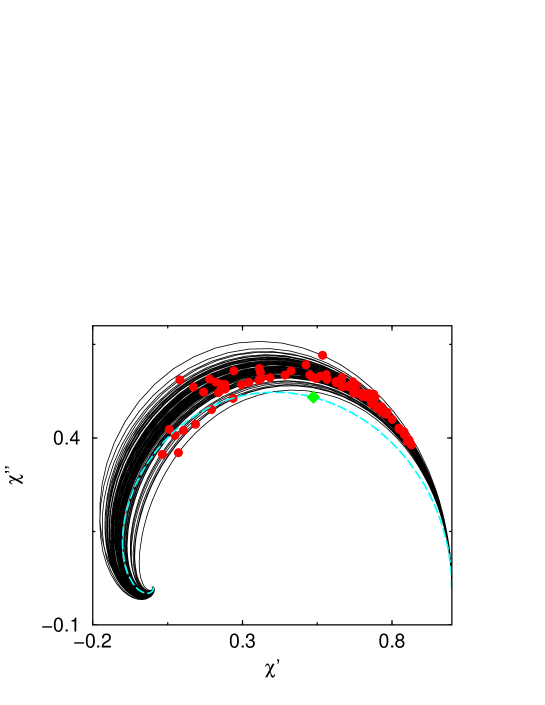
Figure 10: The Cole-Cole plots of the admittances when the exponent of the probability distribution of jump rates is $\alpha=1.0$ and $N=100$. Solid lines represent the admittances for each of 30 samples. The dashed line represents the admittance averaged over 5000 samples. The red solid circles represent the admittance of each sample at $\tilde{\omega}=0.68$. The green diamond which denotes the averaged admittance at $\tilde{\omega}=0.68$ exists at different position from that of the red solid circles.

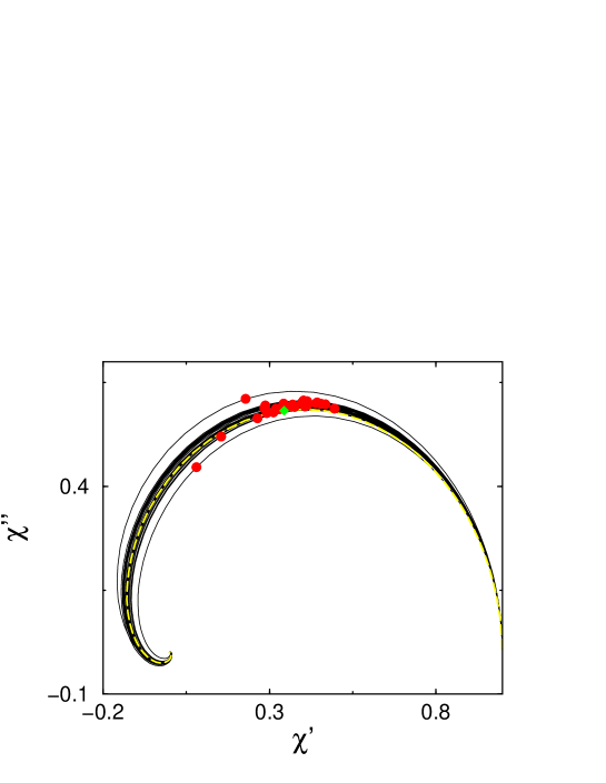
Figure 11: The Cole-Cole plots of the admittances when $\alpha=1.5$ and $N=100$. Solid lines represent the admittances for each of 30 samples. The yellow dashed line represents the admittance averaged over 5000 samples. The red solid circles represent the admittance of each sample at $\tilde{\omega}=1.0$. The green diamond denotes the averaged admittance at $\tilde{\omega}=1.0$. In contrast to the strongly disordered case Fig. 9, the circles concentrate in small region and the solid lines lie almost on the dashed line.

This property of the angle $\theta$ is derived from the regular behavior as $\langle\chi\rangle-1\sim i\tilde{\omega}$ (see Eq. (17) and Eq. (18).).

It is important to note that Fig. 10 suggests that the complex admittance is non-self-averaging when $\alpha=1$. One sees that the disorder-averaged complex admittance $\langle\chi\rangle$ exists at different position from that of the complex admittance for each samples. Although it was shown that the low frequency behavior is self-averaging, it seems that the complex admittance at the finite frequency is non-self-averaging. Consequently, we conclude that the complex admittance is non-self-averaging when $0<\alpha\leq 1$.

VI Understanding of non-self-averaging of the complex admittance with a toy model

In the previous section, we discussed absence of self-averaging for the admittance when disorder of the jump rates is strong. In this section, in order to consider the conditions for absence of self-averaging we introduce a simple model, which is a toy version of the complex admittance and can be analyzed rigorously. This simple model will provide understanding of the reason why the admittance is non-self-averaging, since absence of self-averaging for the simple model is shown below with the same discussion as employed in the analysis of the complex admittance.

Analysis of the admittance is difficult because it does not consist of a mean of independent and identically distributed random variables. Hence, we consider a toy model of the admittance which is a simple function of a mean of independent and identically distributed random variables given by

$$\epsilon_{N}(\omega)\equiv\frac{1}{1+i\omega\sum^{N}_{i=1}(1/w_{i})/N}.$$ (23)

We call it the dielectric constant. It is obvious that the Cole-Cole plot of each sample is the Debye semi-circle since the form of Eq. (23) is the same as that of the dielectric constant of the Debye relaxation. In addition, since $|\epsilon_{N}(\omega)|$ is less than unity, $\epsilon_{N}(\omega)$ is finite for any set of the random jump rates ${w_{i}}$.

In the analyses presented below, we use the following theorems of probability theory Feller66 summarized in appendix .1; Let $\{x_{i}\}$ be a set of independent and identically distributed random variables.

Theorem VI.1 (Law of large numbers)

When the expectation value $\langle x_{i}\rangle$ exists, law of large numbers holds, i.e.

$$Prob\left(\left|\frac{\sum_{i=1}^{N}x_{i}}{N}-\langle x_{j}\rangle\right|>\epsilon\right)\rightarrow 0\ \mbox{as $N\rightarrow\infty$}.$$ (24)

Theorem VI.2 (Corollary of the extended central limit theorem)

When the expectation value $\langle x_{i}\rangle$ diverges, in order that the probability distribution of $\sum_{i=1}^{N}x_{i}/a_{N}-b_{N}$ converges as $N\rightarrow\infty$ it is necessary that the probability density $\rho(x_{i})$ is of the form

$$\rho(x)\sim x^{-\alpha-1}L(x)$$ (25)

for $0<\alpha\leq 1$. Here, $L(x)$ is a slowly varying positive function which is precisely defined by Eq. (73). The normalization constant $a_{N}$ is chosen so that

$$N\frac{L(a_{N})}{{a_{N}}^{\alpha}}\rightarrow C$$ (26)

as $N\rightarrow\infty$.

• When $0<\alpha<1$ in Eq. (25), the probability distribution of $\sum x_{i}/a_{N}$ converges to the stable distribution with the characteristic exponent $\alpha$.

• When $\alpha=1$ in Eq. (25), the probability distribution of $\sum x_{i}/a_{N}-b_{N}$ converges to the stable distribution with the characteristic exponent $\alpha=1$. The centering constant $b_{N}$ diverges as $N\rightarrow\infty$ footnote2 .

By using these theorems, we discuss sample-dependence of the dielectric constant $\epsilon(\omega)\equiv\lim_{N\rightarrow\infty}\epsilon_{N}(\omega)$. The discussion is divided into two parts: the case where the expectation value $\langle 1/w_{i}\rangle$ is finite and the case where the expectation value diverges.

When the expectation value $\langle 1/w_{i}\rangle$ is finite, it is shown from law of large numbers that

$$\epsilon(\omega)\equiv\lim_{N\rightarrow\infty}\frac{1}{1+i\omega\sum_{i=1}^{N}(1/w_{i})/N}=\frac{1}{1+i\omega\langle 1/w_{i}\rangle}.$$ (27)

Thus, there is no sample-dependence, i.e. the dielectric constant is self-averaging in the limit $N\rightarrow\infty$. It is obvious that the Cole-Cole plot is the Debye semi-circle, which corresponds to the Cole-Cole plot of the dielectric constant for each sample.

When the expectation value $\langle 1/w_{i}\rangle$ diverges (strong disorder), we discuss below the two cases of the value of $\alpha$ in Eq. (25): $0<\alpha<1$ and $\alpha=1$. In order to see frequency dependence of $\epsilon(\omega)$, the macroscopic limit ($N\rightarrow\infty$) should be taken so that $\omega\sum 1/w_{i}/N$ is finite. Otherwise, $\epsilon(\omega)$ becomes a constant $0$ or $1$.

• When $0<\alpha<1$, from the extended central limit theorem, $\tilde{T}\equiv\lim_{N\rightarrow\infty}\sum 1/w_{i}/a_{N}$ is a random variable with a limiting probability distribution and hence it is finite with probability one. Hence, the limit $N\rightarrow\infty$ should be taken so that $\omega a_{N}/N$ is finite;

  $$\epsilon(\omega) \equiv \lim_{{N\rightarrow\infty}\atop{\;\tilde{\omega}=\omega a_{N}/N}}\frac{1}{1+i\omega\sum(1/w_{i})/N}$$ (28)

  $$= \lim_{{N\rightarrow\infty}\atop{\;\tilde{\omega}=\omega a_{N}/N}}\frac{1}{1+i\omega a_{N}/N\sum(1/w_{i})/a_{N}}$$

  $$= \frac{1}{1+i\tilde{\omega}\tilde{T}}.$$

  It implies that the frequency-dependence is scaled with $\omega a_{N}/N$ as shown in Fig. 12.

  

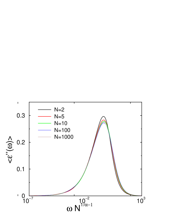
  Figure 12: The frequency-dependence of the imaginary part of the disorder-averaged dielectric constant when the probability distribution function of the jump rates is power-law $\rho(w_{i})=\alpha w_{i}^{\alpha-1}\ (\alpha=1/2$). The two curves for sufficiently long chains $N=100,1000$ lie on the same curve when plotted as a function of the scaled frequency $\omega N^{1/\alpha-1}$ ($\alpha=1/2$).

  Since $\tilde{T}$ is a random variable, $\epsilon(\omega)$ is also a random variable and hence $\epsilon(\omega)$ is non-self-averaging. In addition, since it is known that the probability density $\rho(x)$ of a stable distribution with characteristic exponent $\alpha$ behaves asymptotically as $\rho(x)\sim x^{-\alpha-1}$, the probability density $\rho(\tilde{T})$ behaves as $\rho(\tilde{T})\sim{\tilde{T}}^{-\alpha-1}$. Hence, the expectation value $\langle\tilde{T}\rangle$ diverges. Since it implies that the coefficient of the first order of low $\tilde{\omega}$ expansion diverges, the disorder-averaged dielectric constant is a non-analytic function of $i\ \tilde{\omega}$ which must behave as $\langle\epsilon(\omega)\rangle-1\sim(i\ \tilde{\omega})^{\mu}\ (0<\mu<1)$. Thus, from the same argument employed in the discussion for the Cole-Cole plot of the admittance in Sec. V the Cole-Cole plot of the disorder-averaged dielectric constant appears inside the Debye semi-circle which corresponds to the Cole-Cole plot of the dielectric constant for each sample (see Fig. 13).

  

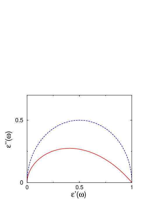
  Figure 13: The Cole-Cole plot of the disorder-averaged dielectric constant (solid line) when $w_{i}$ are random jump rates with the power-law distribution Eq. (12) with $\alpha=1/2$ and the Debye semi-circle (dashed line). It is seen that the Cole-Cole plot of the disorder-averaged dielectric constant is inside the Cole-Cole plot for each sample, i.e. the Debye semi-circle.

• When $\alpha=1$, from the extended central limit theorem, $\sum 1/(w_{i})/a_{N}-b_{N}$ is a random variable with a limiting probability distribution and hence it is finite with probability one. Furthermore, $b_{N}$ diverges as $N\rightarrow\infty$ as shown in appendix .2. Hence, the limit $N\rightarrow\infty$ should be taken so that $\omega a_{N}b_{N}/N$ is finite;

  $$\epsilon(\omega) \equiv \lim_{{N\rightarrow\infty}\atop{\;\tilde{\omega}=\omega a_{N}b_{N}/N}}\frac{1}{1+i\omega\sum(1/w_{i})/N}$$ (29)

  $$= \lim_{{N\rightarrow\infty}\atop{\;\tilde{\omega}=\omega a_{N}b_{N}/N}}\frac{1}{1+i\omega a_{N}b_{N}/N\left[\left(\sum(1/w_{i})/a_{N}-b_{N}\right)/b_{N}+1\right]}$$

  $$= \frac{1}{1+i\tilde{\omega}}.$$

  Hence, $\epsilon(\omega)$ is self-averaging.

Consequently, we conclude that only when $0<\alpha<1$ the dielectric constant is non-self-averaging.

In order to test the foregoing discussion, we present an example of the above analysis where the random jump rates distributed by the power-law distribution Eq. (12) when $\alpha=1/2$. From the extended central limit theorem, it is known that the distribution function of $\tilde{T}$ is given by the stable distribution with $\alpha=1/2$. From Eq. (83), the probability distribution $g(\tilde{T})$ of $\tilde{T}$ behaves as $g(\tilde{T})\sim{\tilde{T}}^{-3/2}$. Hence, when $\tilde{\omega}\simeq 0$ the disorder-averaged dielectric constant behave as

$$\langle\epsilon(\omega)\rangle-1\sim\sqrt{i\tilde{\omega}}.$$ (30)

On the other hand, the dielectric constant for each sample behaves as

$$\epsilon(\omega)-1\sim i\tilde{\omega}.$$ (31)

Thus, the low-frequency behavior is non-self-averaging. Absence of self-averaging is also seen in the Cole-Cole plot (Fig. 13).

VII Higher dimensional disordered media

It is important to note that the system treated above is purely one-dimensional and it is still an open problem whether the admittance for higher dimensional media is self-averaging.

In this section, we investigate properties of the admittance for higher dimensional disordered media in the same manner for one-dimensional media. At first, the statistics of the MFPT for higher dimensional media is analyzed analytically. With the results, it is shown that the complex admittance is non-self-averaging. After that, the theoretical results are confirmed numerically.

For its feasibility, we investigate a site-disordered model called the random trap model, which is defined as a random walk model where the jump rate $w_{i\ j}$ from site $j$ to site $i$ depends only on $j$.

We assume that the higher dimensional medium is a $N\times M$ square (or cubic) lattice. Here, $N$ is the linear dimension of the medium in direction of the current and a number of grid points on the cross section perpendicular to the current direction is denoted as $M$. The periodic boundary condition on the side ends is assumed, i.e., the medium is a hyper-cylinder, and the oscillatory input current is introduced uniformly on the left end of the medium. An example of two-dimension is illustrated in Fig. 14.

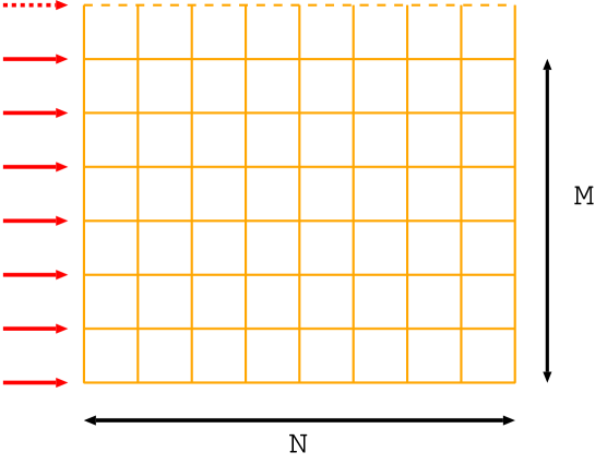
Figure 14: The schematic picture of the two-dimensional medium with an oscillatory input current.

The probability distribution for the jump rates is assumed power-law distribution Eq. (12) with the exponent $\alpha$. Since we are interested in amorphous semiconductors, our analyses are limited to the case $0<\alpha<1$.

VII.1 The analytic expression for the MFPT of higher dimensional media

At first, we introduce a general analytical expression for the MFPT in terms of the backward equation. After that, by using the expression, the results for the one-dimensional MFPT and the extended central limit theorem, the probability distribution of the higher-dimensional MFPT is investigated. Since the analyses are general, results are applicable both to two-dimensional and three-dimensional media.

The backward equation, i.e., the time-development equation for a averaged quantity, is derived in the following way.

Let $P_{\mathbf{j}\mathbf{i}}(t)$ be the probability that the random walker starting from the site $\mathbf{i}$ at time $0$ is found at the site $\mathbf{j}$ at time $t$. We assume that the master equation for the probability is written as

$$\dot{\mathbf{P_{\mathbf{i}}}}(t)=H\mathbf{P_{\mathbf{i}}}(t).$$ (32)

Here, $\mathbf{P_{\mathbf{i}}}$ is the vector whose $\mathbf{j}$-th component is $P_{\mathbf{j}\mathbf{i}}$ with fixing the starting site $\mathbf{i}$. Furthermore, $H$ is a linear operator given in terms of the jump rates.

We consider the time-development equation of the average of the site-dependent quantity $f_{\mathbf{j}}$. The average $g_{\mathbf{i}}$ is defined by

$$g_{\mathbf{i}}(t)\equiv\sum_{\mathbf{j}}f_{\mathbf{j}}P_{\mathbf{j}\mathbf{i}}(t)$$ (33)

and hence the time-derivative is written as

$$\dot{g}_{\mathbf{i}}(t)=\sum_{\mathbf{j}}f_{\mathbf{j}}\dot{P}_{\mathbf{j}\mathbf{i}}(t)=\sum_{\mathbf{j}\mathbf{k}}f_{\mathbf{j}}H_{\mathbf{j}\mathbf{k}}P_{\mathbf{k}\mathbf{i}}(t).$$ (34)

Taken the limit $t\rightarrow 0$,

$$\dot{g}_{\mathbf{i}}(0)=\sum_{\mathbf{j}\mathbf{k}}f_{\mathbf{j}}H_{\mathbf{j}\mathbf{k}}\delta_{\mathbf{k}\mathbf{i}}=\sum_{\mathbf{j}}f_{\mathbf{j}}H_{\mathbf{j}\mathbf{i}}=\sum_{\mathbf{j}}\left({}^{t}H\right)_{\mathbf{i}\mathbf{j}}f_{\mathbf{j}}.$$ (35)

Let $\mathbf{g}(t)$ be the vector whose component is $g_{\mathbf{i}}(t)$, then

$$\dot{\mathbf{g}(0)}=^{t}H\mathbf{f}.$$ (36)

By using the above result, $\mathbf{g}(t)$ is Maclaurin-expanded as

$$\mathbf{g}(t)=\sum_{n=0}^{\infty}\frac{1}{n!}\mathbf{g}^{(n)}(0)t^{n}=\sum_{n=0}^{\infty}\frac{1}{n!}(^{t}H)^{n}\mathbf{f}t^{n}.$$ (37)

Taken the time-derivative,

$$\dot{\mathbf{g}}(t)=\sum_{n=1}^{\infty}\frac{n}{n!}(^{t}H)^{n}\mathbf{f}t^{n-1}=^{t}H\sum_{n=0}^{\infty}\frac{1}{n!}^{n}\mathbf{f}t^{n}=^{t}H\mathbf{g}(t).$$ (38)

The last equality gives the backward equation:

$$\dot{\mathbf{g}}(t)=^{t}H\mathbf{g}(t).$$ (39)

As an example of the average $g_{\mathbf{i}}(t)$, we consider the probability that the random walker staring at the site $\mathbf{i}$ on the end illuminated with the laser light is found in the medium at the time $t(>0)$. The survival probability $n_{\mathbf{i}}(t)$ is defined as

$$n_{\mathbf{i}}(t)\equiv\sum_{\mathbf{j}}P_{\mathbf{j}\mathbf{i}}(t).$$ (40)

Since the probability can be considered as a averaged quantity, $n_{\mathbf{i}}(t)$ obeys the backward equation:

$$\dot{\mathbf{n}}(t)=^{t}H\mathbf{n}(t),$$ (41)

where $\mathbf{n}(t)$ is the vector whose component is $n_{i}(t)$.

In terms of the survival probability, the first passage time distribution (FPTD) $F(t)$ is written as

$$F(t)=-\frac{d}{dt}\sum_{\mathbf{i}}n_{\mathbf{i}}(t)/M,$$ (42)

where $M\equiv\sum_{\mathbf{i}}1$ and the sum is taken over the grid points on the end of the medium. Hence, the MFPT $\bar{t}$ is also written as

$$\bar{t}\equiv\int^{\infty}_{0}tF(t)dt=-\frac{1}{M}\sum_{\mathbf{i}}\int_{0}^{\infty}t\frac{d}{dt}n_{\mathbf{i}}(t)dt=\frac{1}{M}\sum_{\mathbf{i}}\int_{0}^{\infty}n_{\mathbf{i}}(t)dt=\frac{1}{M}\tilde{n}_{\mathbf{i}}(0).$$ (43)

Here, $\tilde{n}_{\mathbf{i}}(0)$ is the limit $s\rightarrow 0$ of the Laplace transform $\tilde{n}_{\mathbf{i}}(s)$. The Laplace-transform of the backward equation is written as

$$s\tilde{\mathbf{n}}(s)-\mathbf{n}(t=0)=^{t}H\tilde{\mathbf{n}}(s).$$ (44)

Taken the limit $s\rightarrow 0$,

$${}^{t}H\tilde{\mathbf{n}}(0)=-\mathbf{n}(t=0),$$ (45)

where $\mathbf{n}(t=0)=^{t}(1,1,\cdots)$. By solving Eq. (45), the MFPT is obtained as Eq. (43).

In the rest of this section, we concentrate on the random trap model. For the $d$-dimensional random trap model, the analytical expression of the MFPT can be easily obtained by Eq. (45) in the following way.

Each components in the same column of the matrix $H$ are written only in terms of the jump rates of the same site. It means that each components in the same line of the transposed matrix ${}^{t}H$ are written only with the jump rates of the same site. Hence, divided the each lines of Eq. (45) by the jump rates, we obtain

$${}^{t}H_{0}\tilde{\mathbf{n}}(0)=-\left(\begin{array}[]{c}\vdots\\ 1/w_{\mathbf{k}}\\ \vdots\end{array}\right).$$ (49)

Here, ${}^{t}H_{0}$ is the transpose of the time-development operator when the jump rates of the all sites are equal to unity. From Eq. (49), $\tilde{\mathbf{n}}(0)$ is a homogeneous linear function of the inverse of the jump rates.

We denote the grid points in $d$-dimensional medium with two indexes, $n$ and $\mathbf{m}$. One index $n$ is the label of the cross sections normal to the current direction and the other index $\mathbf{m}$ is the $d-1$ dimensional vector to denote a grid point on the cross section. Let the cross section at the left end, which is illuminated with laser light, be numbered $0$ and the cross section at the right end be numbered $N-1$. Each cross sections have $M$ grid points.

Since the boundary condition at the side ends is periodic, each grid points in the same cross section are identical geometrically and each jump rates $w_{n\mathbf{m}}$ in the same cross section $n$ have the same contribution to the MFPT. Hence, the results obtained above means that the MFPT for the $d$-dimensional medium, $\bar{t}_{d}$ is written as

$$\bar{t}_{d} = \frac{1}{M}\sum_{\mathbf{m}}\sum_{n=0}^{N-1}\frac{a_{n}}{w_{n\mathbf{m}}}$$ (50)

$$= \frac{1}{M}\sum_{\mathbf{m}}\left(\frac{a_{0}}{w_{0\mathbf{m}}}+\frac{a_{1}}{w_{1\mathbf{m}}}+\cdots+\frac{a_{N-1}}{w_{N-1\mathbf{m}}}\right),$$

where $\{a_{n}\}$ are constants independent of configuration of disorder. If all the jump rates in a cross section are equal, i.e., $w_{n\mathbf{m}}=w_{n\mathbf{m}^{\prime}}\equiv w_{n}$, the $d$-dimensional MFPT $\bar{t}_{d}$ is equal to the one-dimensional MFPT $\bar{t}_{1}$, which is given as

$$\bar{t}_{1}=\frac{N}{w_{0}}+\frac{N-1}{w_{1}}+\cdots+\frac{1}{w_{N-1}}.$$ (51)

Comparison of Eq. (50) to Eq. (51) shows that

$$a_{n}=N-n.$$ (52)

Consequently, the MFPT for $d$-dimensional medium is given as

$$\bar{t}_{d} = \frac{1}{M}\sum_{\mathbf{m}}\sum_{n=0}^{N-1}\frac{N-n}{w_{n\mathbf{m}}}$$ (53)

$$= \frac{1}{M}\sum_{\mathbf{m}}\left(\frac{N}{w_{0\mathbf{m}}}+\frac{N-1}{w_{1\mathbf{m}}}+\cdots+\frac{1}{w_{N-1\mathbf{m}}}\right).$$

With respect to the MFPT, the $d$-dimensional medium is a bundle of one-dimensional chain and hence the MFPT is rewritten as

$$\bar{t}_{d}=\frac{1}{M}\sum_{\mathbf{m}}t^{(\mathbf{m})}_{1},$$ (54)

where $t^{(\mathbf{m})}_{1}$ is the MFPT for a one-dimensional medium defined as

$$t^{(\mathbf{m})}_{1}\equiv\sum_{n=0}^{N-1}\frac{N-n}{w_{n\mathbf{m}}}.$$ (55)

VII.2 The statistics of the MFPT for higher dimensional media

In order to consider the probability distribution of $\bar{t}_{d}$, the following postulate, which is expected to be true from the results of analyses for the one-dimensional case, is introduced: Let $\{u_{n}\}$ be a set of independent and identically distributed random variables. The tail of the probability density is assumed to be

$$\rho_{u}(u_{n})\sim{u_{n}}^{-\alpha-1},$$ (56)

where $0<\alpha<1$. Then, we postulate that the random variable $v$ defined as

$$v\equiv\frac{1}{N^{1/\alpha+1}}\sum_{n=0}^{N-1}(N-n)u_{n}$$ (57)

has a normalized probability distribution function and the tail obeys the power law.

By making use of the postulate, we analyze the statistics of $\bar{t}_{d}$ in two different ways and determine the asymptotic form of the probability distribution of $\bar{t}_{d}$.

At first, we take the way where the sum in terms of $n$ is done first. From our postulate, the random variable $\tilde{t}_{\mathbf{m}}$ defined as

$$\tilde{t}_{\mathbf{m}}\equiv\frac{1}{N^{1/\alpha+1}}t^{(\mathbf{m})}_{1}$$ (58)

has the normalized probability distribution function and it obeys the power law:

$$\rho_{\tilde{t}}(\tilde{t}_{\mathbf{m}})\sim{\tilde{t}_{\mathbf{m}}}^{-\alpha^{\prime}-1},$$ (59)

where $\alpha^{\prime}$ is a positive constant. Since $\bar{t}_{d}=M^{-1}N^{1/\alpha+1}\sum_{\mathbf{m}}\tilde{t}_{\mathbf{m}}$, from the extended central limit theorem, the random variable $x$ defined as

$$x\equiv\frac{1}{M^{1/\alpha^{\prime}-1}N^{1/\alpha+1}}\bar{t}_{d}$$ (60)

has a normalized probability distribution function and its tail asymptotically behaves as

$$\rho_{x}(x)\sim x^{-\alpha^{\prime}-1}.$$ (61)

As the other way, we evaluate the sum in terms of $\mathbf{m}$ first. The extended central limit theorem shows that the random variable $y_{n}$ defined as

$$y_{n}\equiv\frac{1}{M^{1/\alpha}}\sum_{\mathbf{m}}\frac{1}{w_{n\mathbf{m}}}$$ (62)

has a normalized probability distribution function whose asymptotic form is

$$\rho_{y}(y_{n})\sim{y_{n}}^{-\alpha-1}.$$ (63)

Furthermore, since $\bar{t}_{d}=M^{1/\alpha-1}\sum_{n=0}^{N-1}(N-n)y_{n}$, our postulate means that the random variable $z$ defined as

$$z\equiv\frac{1}{M^{1/\alpha-1}N^{1/\alpha+1}}\bar{t}_{d}$$ (64)

has a probability distribution function whose tail behaves as

$$\rho_{z}(z)\sim z^{-\alpha-1}.$$ (65)

Here, we compare the two ways of normalization Eqs. (60), (64). Since the two ways of normalization to obtain the normalized distribution function should be identical,

$$\alpha^{\prime}=\alpha.$$ (66)

Summarized our results, the MFPT $\bar{t}_{d}$ is normalized as

$$\bar{t}_{d}\equiv M^{1/\alpha-1}N^{1/\alpha+1}z$$ (67)

and the probability distribution function has the power-law tail as

$$\rho_{z}(z)\sim z^{-\alpha-1}.$$ (68)

Furthermore, from Eq. (66), the tail of the probability distribution function of $v$ defined by Eq. (57) behaves as

$$\rho_{v}(v)\sim v^{-\alpha-1}.$$ (69)

Since the results are based on the postulate, we confirm numerically them. Figure 15 shows that the probability distribution function of $z$ converges to a unique distribution when $N$ and $M$ are increased. The power-law tail of the distribution is shown in Fig. 16. It is clearly seen that the exponent is equal to $-1.5$ when $\alpha=0.5$.

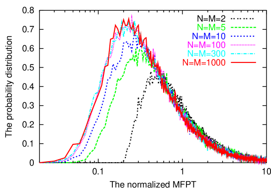
Figure 15: The probability distribution function of the normalized MFPT $\bar{t}_{d}N^{-1/\alpha-1}M^{-1/\alpha+1}$ for the random trap model where the probability distribution function of the random jump rates is power-law Eq. (12) with exponent $\alpha=1/2$. The distribution is computed from 100000 samples of the length and width $N,M=2,5,10,100,300,1000$. It is clearly seen that the probability distribution functions lie on a same curve when the length of lattice $N$ is sufficiently large.

Figure 16: The asymptotic behavior of the probability distribution function of the normalized MFPT computed from 1000000 samples. The solid line denotes the distribution function when $N=M=100$ and $\alpha=1/2$ and the dashed line represents the function proportional to $z^{-1.5}$. One sees clearly that the distribution function behaves asymptotically as $\rho_{z}(z)\sim z^{-\alpha-1}(-\alpha-1\simeq 1.5<2).$

VII.3 Non-self-averaging complex admittances for higher dimensional media

By using the results obtained in the previous subsection, Eqs. (67), (68), we show in the same way as for the one-dimensional case that the complex admittance for higher dimensional media is also non-self-averaging when $0<\alpha<1$.

The normalization of the MFPT, Eq. (67), means that the complex admittance for an infinitely large higher dimensional medium is given as

$$\lim_{N,M\rightarrow\infty}\chi_{N,M}(\omega)=1-iz\tilde{\omega}+\ldots$$ (70)

in terms of the scaled frequency $\tilde{\omega}$ defined as

$$\tilde{\omega}\equiv\omega M^{1/\alpha-1}N^{1/\alpha+1}.$$ (71)

Here, the infinite volume limit $N,M\rightarrow\infty$ is taken with fixing $\tilde{\omega}$ at a finite value. Since the normalized MFPT $z$ is a random number, the complex admittance is dependent on each samples even for the infinitely large medium. That is, the complex admittance is non-self-averaging.

Furthermore, from Eq. (68), it is shown that $\langle z\rangle=\infty$. It means non-analyticity of the complex admittance about $\tilde{\omega}=0$ and hence

$$\langle\lim_{N,M\rightarrow\infty}\chi_{N,M}(\omega)\rangle-1\sim(i\tilde{\omega})^{\mu},$$ (72)

where $\mu$ is a constant such that $0<\mu<1$ (see Fig. 17).

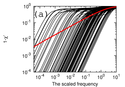
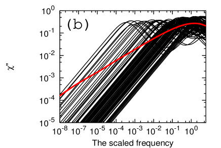
Figure 17: The frequency dependence of the real part (a) and the imaginary part (b) of the complex admittances for two-dimensional media when the exponent of the probability distribution of jump rates is $\alpha=1/2$ and the size of the media is $N=M=10$. The thin solid lines represent the admittances for each of 100 samples. The bold solid line represents the admittance averaged over 20000 samples. Though the admittance of each sample is proportional to the scaled frequency $\tilde{\omega}$, the averaged admittance is proportional to $\sqrt{\tilde{\omega}}$ ($\mu\simeq 1/2$).

The results obtained above are all concerned with the low frequency behavior. We investigate numerically the non-self-averaging characteristics in the all frequency range with the Cole-Cole plot. Figure 18 shows the Cole-Cole plots of the admittances for one hundred realizations of $4\times 4,10\times 10,30\times 30$ square lattices. These numerical results show that the sample-dependence of the admittance seems to exist even when both the length of the lattice and the width are large and hence it implies that the admittance is non-self-averaging even in higher dimensional cases.

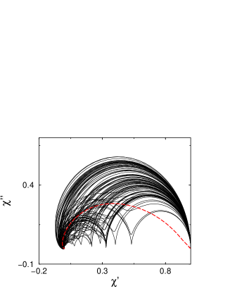
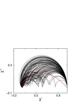
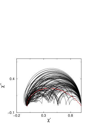
Figure 18: (a) The Cole-Cole plot for $4\times 4$ disordered square lattice. The probability distribution for the jump rates is power-law distribution Eq. (12) when $\alpha=1/2$. The solid lines denote admittances for 100 samples and the dashed line denotes the admittance disorder-averaged over 5000 samples. (b) The Cole-Cole plot for $10\times 10$ disordered square lattice. (c) The Cole-Cole plot for $30\times 30$ disordered square lattice. These numerical results show that the sample-dependence of the admittance seems to exist even when the size of the lattice is large and hence it means that the admittance is non-self-averaging.

VIII Discussion and conclusions

In conclusion, we presented a generic stochastic dynamical model in one-dimensional medium of the BPM and showed that the admittance has important information about transport in disordered media, e.g. the FPTD. Thus, the BPM will be a powerful technique to investigate the dynamical process in random media. We also showed that the admittance is non-self-averaging when the jump rates are random variables with the power-law distribution as $\rho(w_{i})\sim{w_{i}}^{\alpha-1}\ (0<\alpha\leq 1)$. It is important to note that this power-law distribution is realized in amorphous semiconductors.

On the other hand, when $1\leq\alpha$, the low frequency behavior of $O(\omega)$ has no sample dependence as shown in Eqs. (17), (18). However, with respect to the terms of $O(\omega^{2})$, the second moment of the inverse of the jump rate $\langle 1/w^{2}\rangle$, which diverges when $1\leq\alpha\leq 2$, is concerned. It implies that some anomalous statistical properties may be observed. Properties for the full frequency range were analyzed with the Cole-Cole plots. In the marginal case when $\alpha=1$, the non-self-averaging property appears as shown in Fig. 10. However, Fig. 11 shows that such effects from terms of $O(\omega^{2})$ are small when $1<\alpha$.

When the complex admittance is non-self-averaging, the behavior of the averaged admittance over infinite number of samples does not coincide with that of the admittance observed in experiments. In order to see the non-self-averaging behavior described above one needs to work in one-dimensional system or the case where the translational invariance is violated in only one direction.

Furthermore, in order to investigate possibility that the non-self-averaging properties of the admittance are observed in real experiments on higher dimensional media, we performed theoretical and numerical analyses of the admittance on higher dimensional disordered media. The analyses on anomalous statistics of the MFPT show that the non-self-averaging characteristics are observed in the low-frequency behavior of the complex admittance of higher-dimensional media. The numerical results confirm the conclusion that the admittance is non-self-averaging. Hence, it suggests possibility that the non-self-averaging properties of the admittance of the BPM may be observed in the real experiments on higher dimensional media.

On the other hand, non-self-averaging behavior, i.e. strong sample-dependence may be observed in other experiments. For example, it is known that anomalous system-size dependence of the mobility, $\mu\sim L^{1-1/\alpha}$, is observed in the time-of-flight experiment of amorphous semiconductors Pfister78 . The anomalous system-size dependence is due to the fact that the smallest value of random jump rates depends on the length of a chain Kehr98 . Since the smallest value dominates the mobility, the mobility is also a random variable. Thus, the anomalous system-size dependence of the mobility implies that the mobility is not self-averaging.

Law of large numbers and the extended central limit theorem

In this appendix, we summarize the notions of probability theory, partly rewritten for our convenience, used to analyze the complex admittance and the “dielectric constant” in Secs. V and VI. After that, we show that $b_{N}$ Eq. (13) diverges as $N\rightarrow\infty$.

.1 The extended central limit theorem

Here, we summarize theorems on probability distribution of normalized sum of random variables Feller66 .

The following law of large numbers tells that a mean converges to an expectation value even when a variance does not exist. In this section, $S_{n}$ denotes the sum $\sum_{i=1}^{n}X_{i}$.

Theorem .1 (Strong law of large numbers)

Let the $X_{k}$ be independent random variables with a common distribution $F$. If they have an expectation $\mu$ then $S_{n}/n\rightarrow\mu$ with probability one.

In order to describe the extended central limit theorem, some concepts are defined.

Definition .1 (Domain of attraction)

The distribution $F$ of the independent random variables $X_{k}$ belongs to the domain of attraction of a distribution $R$ if there exist the norming constant $a_{n}>0$ and the centering constant $b_{n}$ such that the distribution of $a_{n}^{-1}S_{n}-b_{n}$ tends to $R$.

Definition .2 (Slow variation)

A positive function $L$ defined on $(0,\infty)$ varies slowly at infinity if

$$\frac{L(st)}{L(s)}\rightarrow 1$$ (73)

for each $t>0$ as $s\rightarrow\infty$.

It implies that the leading term of $L(st)$ is $L(s)$ when $s$ is large. Constant functions and $\log(x)$ are examples.

In addition, the function $F(x)$ is assumed to be related to the probability density $\rho(x)$ as

$$F(x)\equiv\int_{-\infty}^{x}dy\rho(y).$$ (74)

Using definitions presented above, the extended central limit theorem is stated as follows:

Theorem .2 (The extended central limit theorem)

In order that $F$ belongs to some domain of attraction it is necessary that $F$ is of the form

$$1-F(x)+F(-x)\sim x^{-\alpha}L(x)$$ (75)

for some $0<\alpha\leq 2$ as $x\rightarrow\infty$.

• If $\alpha=2$ then $F$ belongs to the domain of attraction of the normal distribution.

• If $\alpha<2$ and

  $$\frac{1-F(x)}{1-F(x)+F(-x)}\rightarrow p,\ \frac{F(-x)}{1-F(x)+F(-x)}\rightarrow q$$ (76)

  as $x\rightarrow\infty$ then $F$ belongs to the domain of attraction of the stable distribution with the characteristic exponent $\alpha$. If Eq. (76) fails then $F$ belongs to no domain of attraction.

Here, Eq. (76) only means that the limits exist. If positive random variables are considered, $p=1$ and $q=0$ since $F(-x)=0$. The limits $p$ and $q$ give parameters of a stable distribution. In addition, the centering parameter $b_{n}$ is given as followings;

• If $\alpha>1$ then $b_{n}$ is given by the expectation value.

• If $\alpha=1$ then $b_{n}$ is given by

  $$b_{n}=n\int_{-\infty}^{\infty}dx\sin\left(\frac{x}{a_{n}}\right)\rho(x).$$ (77)

• If $\alpha<1$ then $b_{n}=0$.

The norming constant $a_{n}$ is chosen so that

$$\frac{n}{{a_{n}}^{\alpha}}L(a_{n})\rightarrow C,$$ (78)

where $C>0$ is a constant.

This theorem implies that when the disorder is strong and the probability distribution function of the normalized sum $S_{n}/a_{n}-b_{n}$ converges in the limit $n\rightarrow\infty$ the limiting probability distribution is the stable distribution with the characteristic exponent $0<\alpha\leq 1$ given by Eq. (75). The inequality $0<\alpha\leq 1$ is due to divergence of the expectation value (the strong disorder).

For our convenience, we rewrite the necessary condition Eq. (75) for the convergence of the probability distribution of $S_{n}/a_{n}-b_{n}$ in terms of the probability density $\rho(x)$. Since $\rho(x)=F^{\prime}(x)\equiv dF(x)/dx$, the asymptotic behavior of the probability density is given by

$$\rho(x)+\rho(-x)\sim x^{-\alpha-1}L(x)[1-\frac{1}{\alpha}\frac{xL^{\prime}(x)}{L(x)}].$$ (79)

The second term on the right hand side is evaluated from Eq. (73). By differentiation with respect to $t$ of Eq. (73) and setting $t=1$, it is shown that

$$\lim_{s\rightarrow\infty}\frac{L^{\prime}(s)s}{L(s)}=0.$$ (80)

It implies that

$$\rho(x)+\rho(-x)\sim x^{-\alpha-1}L(x)$$ (81)

as $x\rightarrow\infty$.

For the asymptotic behavior of the stable distribution, the following theorem is known.

Theorem .3 (Asymptotic behavior of a stable distribution)

If $G$ is a stable distribution obtained as the limiting distribution of the extended central limit theorem, then as $x\rightarrow\infty$

$$x^{\alpha}[1-G(x)]\rightarrow Cp\frac{2-\alpha}{\alpha},\ x^{\alpha}G(-x)\rightarrow Cq\frac{2-\alpha}{\alpha},$$ (82)

where the parameters $C,p,q$ are given by Eqs. (76) and (78).

It implies that the asymptotic behavior of the probability density $g(x)=G^{\prime}(x)$ is given by

$$g(x)\simeq Cp(2-\alpha)x^{-\alpha-1},\ g(-x)\simeq Cq(2-\alpha)x^{-\alpha-1}.$$ (83)

Hence, a stable distribution with the characteristic exponent $\alpha$ has absolute moments of all orders $<\alpha$ and absolute moments of all orders $\geq\alpha$ do not exist.

Next, we present the relation holding when $0<\alpha<1$. It tells about the contribution of the maximal term to the sum. Let $X_{1},X_{2},\ldots$ be independent random variables with the common distribution $F$ satisfying Eq. (75) with $0<\alpha<1$, i.e., belonging to the domain of attraction of the stable distribution with the characteristic exponent $\alpha$. Put $M_{n}=\max(X_{1},\ldots,X_{n})$. Then,

$$\left\langle\frac{S_{n}}{M_{n}}\right\rangle\rightarrow\frac{1}{1-\alpha}$$ (84)

as $n\rightarrow\infty$. It implies that the maximal term is of the same order as the sum with probability one when $0<\alpha<1$.

.2 The centering constant $b_{n}$ when $\alpha=1$

Here, we show that the centering constant $b_{n}$ diverges for the positive random variables $x$ satisfying Eq. (75) with $\alpha=1$;

$$1-F(x)\sim x^{-1}L(x).$$ (85)

Let $x_{0}>0$ denote the lower limit of the distribution and the probability density is given by $\rho(x)=F^{\prime}(x)$. From Eq. (78), the norming constant $a_{n}$ is chosen so that

$$\frac{n}{a_{n}}L(a_{n})\rightarrow C,$$ (86)

where $C>0$ is a constant. The asymptotic behavior of the probability density $\rho(x)$ is derived from Eq. (81);

$$\rho(x)\sim x^{-2}L(x).$$ (87)

We evaluate $b_{n}$ by dividing the region of integration of Eq. (77);

$$b_{n}=n\int^{x_{n}}_{x_{0}}dx\sin\left(\frac{x}{a_{n}}\right)\rho(x)+n\int^{\infty}_{x_{n}}dx\sin\left(\frac{x}{a_{n}}\right)\rho(x)$$ (88)

where $x_{n}$ is a constant satisfying

$$x_{n}\ll a_{n},\ \ \lim_{n\rightarrow\infty}x_{n}=\infty.$$ (89)

Since $x_{n}\ll a_{n}$, the first term on the right hand side of Eq. (88) is given by

$$\mbox{the first term}\simeq\frac{n}{a_{n}}\int^{x_{n}}_{x_{0}}dxx\rho(x)>0.$$ (90)

From Eq. (87), the leading term of the second term is evaluated as

the second term $$\sim n\int_{x_{n}}^{\infty}dx\sin\left(\frac{x}{a_{n}}\right)x^{-2}L(x)$$ (91)

$$= \frac{n}{a_{n}}\int^{\infty}_{x_{n}/a_{n}}dx\sin\left(x\right)x^{-2}L(a_{n}x),$$

where a numerical constant is ignored. Since $L$ is a function slowly varying, the leading term is given by

the second term $$\sim \frac{n}{a_{n}}L(a_{n})\int^{\infty}_{x_{n}/a_{n}}dx\sin\left(x\right)x^{-2}$$ (92)

$$\sim \frac{n}{a_{n}}L(a_{n})\log(a_{n}).$$

From Eq. (86), it is shown that

$$\mbox{the second term}\sim\log(a_{n}).$$ (93)

Consequently, since the first term is positive and the second term becomes positive infinity in the limit $n\rightarrow\infty$, the centering constant $b_{n}$ diverges in the limit $n\rightarrow\infty$.

References

- (1) The present address: Research Institute for Applied Mechanics, Kyushu University, Kasuga 816-8580, Japan. Electronic address: mituhiro@riam.kyushu-u.ac.jp
- (2) Deceased on Mar. 9, 2000.
- (3) For reviews, see e.g. G. Pfister and H. Scher, Adv. Phys. 27, 747 (1978): F. J. Schmidlin, Philos. Mag. B 41, 535 (1980): H. Scher, M. F. Shlesinger, and J. T. Bendler, Physics Today, January 1991, p. 26.
- (4) M. E. Scharfe, Phys. Rev. B 2, 5025 (1970).
- (5) J. M. López, M. A. Rodríguez, and L. Pesquera, Phys. Rev. E 51, R1637 (1995).
- (6) S. H. Noskowicz and I. Goldhirsch, Phys. Rev. Lett. 61, 500 (1988).
- (7) P. E. de Jongh and D. Vanmaekelbergh, Phys. Rev. Lett. 77, 3427 (1996): G. Franco, J. Gehring, L. M. Peter, E. A. Ponomarev, and I. Uhlendorf, J. Phys. Chem. B 103, 692 (1999).
- (8) G. Pfister and H. Scher, Adv. Phys. 27, 747 (1978).
- (9) M. Kawasaki, T. Odagaki, and K. W. Kehr, Phys. Rev. B 61, 5839 (2000).
- (10) K. P. N. Murthy and K. W. Kehr, Phys. Rev. A 40, 2082 (1989).
- (11) This power-law probability distribution for the jump rates corresponds to the dwell time distribution used in the study of dispersive transport where is proportional to temperature Pfister78 , and it has been shown that the power-law distribution is common for activation processes with random activation energy Odagaki95 .
- (12) T. Odagaki, Phys. Rev. Lett. 75, 3701 (1995).
- (13) S. Alexander, J. Bernasconi, W. R. Schneider, and R.Orbach, Rev. Mod. Phys. 53, 175 (1981): J. W. Haus and K. W. Kehr, Phys. Rep. 150, 263 (1987): G. H. Weiss and R. J. Rubin, Adv. Chem. Phys. 52, 363 (1983): J. P. Bouchaud and A. Georges, Phys. Rep. 195, 127 (1990).
- (14) W. Feller, An introduction to probability theory and its applications volume 2 (John Wiley & Sons, New York, 1966).
- (15) It is shown in appendix .2.
- (16) K. W. Kehr, K. P. N. Murthy, and H. Ambaye, Physica A 253, 9 (1998).