Economic Small-World Behavior in Weighted Networks

Abstract

The small-world phenomenon has been already the subject of a huge variety of papers, showing its appeareance in a variety of systems. However, some big holes still remain to be filled, as the commonly adopted mathematical formulation suffers from a variety of limitations, that make it unsuitable to provide a general tool of analysis for real networks, and not just for mathematical (topological) abstractions. In this paper we show where the major problems arise, and how there is therefore the need for a new reformulation of the small-world concept. Together with an analysis of the variables involved, we then propose a new theory of small-world networks based on two leading concepts: efficiency and cost. Efficiency measures how well information propagates over the network, and cost measures how expensive it is to build a network. The combination of these factors leads us to introduce the concept of economic small worlds, that formalizes the idea of networks that are ”cheap” to build, and nevertheless efficient in propagating information, both at global and local scale. This new concept is shown to overcome all the limitations proper of the so-far commonly adopted formulation, and to provide an adequate tool to quantitatively analyze the behaviour of complex networks in the real world. Various complex systems are analyzed, ranging from the realm of neural networks, to social sciences, to communication and transportation networks. In each case, economic small worlds are found. Moreover, using the economic small-world framework, the construction principles of these networks can be quantitatively analyzed and compared, giving good insights on how efficiency and economy principles combine up to shape all these systems.

]

I INTRODUCTION

There is a revolution in the making when it comes to understanding the complex world around us [1]. For decades we have been taught to look for the source of all complex behaviors in the properties of the system’s simple constituents: the main idea to approach a physical problem was based on the fact that any physical system, even if extreme complicate, would simplify when studied at smaller and smaller scale and divided into many simple systems. In the last years this view has rapidly changed, with the beginning of a broad movement of interests and researches on multidisciplinary problems, and the birth of a new science, the science of complexity [1, 2]. Today, the most accepted definition of a complex system is that of a system made by a large number of interacting elements or components whose collective behavior cannot be simply understood in terms of the behavior of the components. To make few examples of complex systems think of a brain, of a social systems, or of a biological organism. The simple elements of such systems, the neurons in a brain, the people in the social system and the cells in the biological organism are strongly interconnected. Even if we know many things about a neuron or a specific cell, this does not mean we know how a brain or a biological system works: any approach that would cut the system into parts would fail. We need instead mathematical models that capture the key properties of the entire ensemble. Only such approaches can success in describing the non trivial mechanism of how the complex behavior of the whole is related to the behavior of the parts (this aspect is called emergence [1]). The general characteristics of a complex system can be listed as follows:
– The strong interconnection and interdependence of the parts. The elements of a complex system interact in a nonlinear way, and are themselves nonlinear dynamical systems.
– The existence of a rich structure over several scales. In space, this property is the definition of a fractal. In time it means that some process of self-organization is going on, and then the intrinsic order of a complex system is dynamic rather than static.

Therefore, chaos and statistical physics are two mathematical disciplines that have found an intensive application in the study of complex systems. In fact, a complex system can be modelled as a network, where the vertices are the elements of the system and edges represent the interactions between them: neural networks, social interacting species, coupled biological and chemical systems, computer networks or Internet are only few of such examples.

From one side, scientists have concentrated the attention in the study of the dynamics of coupled chaotic systems. Since many things are known about the chaotic dynamics of low-dimensional non linear systems, a great progress has been achieved in the understanding of the dynamical behavior of chaotic systems coupled together in a simple, geometrical regular array (coupled chaotic maps [3]), or in a completely random way [4, 5].

A parallel approach (our paper belongs to this), focuses instead on the architecture of a complex system: it concerns with the study of the connectivity properties of the network. In fact, the network structure can be as important as the nonlinear interactions between elements. An accurate description of the coupling architecture and a characterization of the structural properties of the network can be of fundamental importance also to understand the dynamics of the system. The questions to answer in this case are: how the networks look like, and how do they emerge and evolve. The research about networks has given rather unexpected results: in fact the statistical physics is able to capture the topology of many diverse systems within a common framework, but this common framework is very different from the regular array, or the random connectivity, previously used to model the network of a complex system. In a recent paper Watts and Strogatz have shown that the connection topology of some biological, technological and social networks is neither completely regular nor completely random [6, 7], but stays somehow in between these two extreme cases. These particular class of networks, named small worlds in analogy with the concept of small-world phenomenon developed 30 years ago in social psychology [8], are in fact highly clustered like regular lattices, yet having small characteristic path lengths like random graphs. A pictorial description of this situation is that the networks’ complexity lies at the edge of order and chaos. The original paper of Watts and Strogatz has triggered a large interest on the study of the properties of small worlds (see ref. [9] for a recent review). Researchers have focused their attention on different aspects: study of the inset mechanism [10, 11, 12, 13], dynamics [14] and spreading of diseases on small worlds [15], applications to social networks [16, 17, 18] and to Internet [19, 20].

This paper is about the same definition of the small-world behavior. We show that the study of a generic complex network poses new challenges, that can in fact be overcome by using a more general formalism than the one presented by Watts and Strogatz. The small-world behavior can be defined in a general and more physical way by considering how efficiently the information is exchanged over the network. The formalism we propose is valid both for unweighted and weighted graphs and extends the application of the small-world analysis to any complex network, also to those systems where the euclidian distance between vertices is important and therefore too poorly described only by the topology of connections. The results of our study, in part already been presented in ref.[21], are here extended by the introduction of a new variable quantifying the cost of the network. The paper is organized as follows. In Section II we examine the original formulation proposed by Watts and Strogatz for topological (unweighted) networks. In Section III we present our formalism based on the the global and local efficiency and on the cost of a network: the formalism is valid also for weighted networks. Then we introduce and discuss four simple procedures (models) to construct unweighted and weighted networks. These simple models help to illustrate the concepts of global efficiency, local efficiency and cost, and to discuss the intricate relationships between these three variables. We define an economic small-world network as a low-cost system that communicate efficiently both on a global and on a local scale. In Section IV we present a series of applications to the study of real databases of networks of different nature, origin and size: 1) neural networks (two examples of networks of cortico-cortical connections, and an example of a nervous system at the level of connections between neurons), 2) social networks (the collaboration network of movie actors), 3) communication networks (the World Wide Web and the Internet), 4) transportation systems (the Boston urban transportation systems).

II THE WS FORMULATION

We start by reexamining the “WS formulation” of the small-world phenomenon in topological (relational) networks proposed by Watts and Strogatz in ref. [6]. Watts and Strogatz consider a generic graph $\bf G$ with $N$ vertices (nodes) and $K$ edges (arcs, links or connections). $\bf G$ is assumed to be:

1) Unweighted. The edges are not assigned any a priori weight and therefore are all equal. An unweighted graph is sometimes called a topological or a relational graph, because the difference between two edges can only derive from the relations with other edges.

2) Simple. This means that either a couple of nodes is connected by a direct edge or it is not: multiple edges between the same couple of nodes are not allowed.

3) Sparse. This property means that $K\ll N(N-1)/2$, i.e. only a few of the total possible number of edges $N(N-1)/2$ exist.

4) Connected. $K$ must be small enough to satisfy property 3, but on the other side it must be large enough to assure that there exist at least one path connecting any couple of nodes. For a random graph this property is satisfied if $K\gg N\ln N$.

All the information necessary to describe such a graph are therefore contained in a single matrix $\{a_{ij}\}$, the so-called adjacency (or connection) matrix. This is a $N\cdot N$ symmetric matrix, whose entry $a_{ij}$ is $1$ if there is an edge joining vertex $i$ to vertex $j$, and $0$ otherwise. Characteristic quantities of graph $\bf G$, which will be used in the following of the paper, are the degrees of the vertices. The degree of a vertex $i$ is defined as the number $k_{i}$ of edges incident with vertex $i$, i.e. the number of neighbours of $i$. The average value of $k_{i}$ is $k=1/N~{}\sum_{i}k_{i}=2K/N$. In order to quantify the structural properties of $\bf G$, Watts and Strogatz propose to evaluate two quantities: the characteristic path length $L$ and the clustering coefficient $C$.

A The characteristic path length $L$

One of the most important quantities to characterize the properties of a graph is the geodesic, or the shortest path length between two vertices (popularly known in social networks as the number of degrees of separation [8, 22, 23]). The shortest path length $d_{ij}$ between $i$ and $j$ is the minimum number of edges traversed to get from a vertex $i$ to another vertex $j$. By definition $d_{ij}\geq 1$, and $d_{ij}=1$ if there exists a direct edge between $i$ and $j$. In general the geodesic between two vertices may not be unique: there may be two or more shortest paths (sharing or not sharing similar vertices) with the same length (see ref.[16, 17] for a graphical example of a geodesic in a social system, the collaboration network of physicists). The whole matrix of the shortest path lengths $d_{ij}$ between two generic vertices $i$ and $j$ can be extracted from the adjacency matrix $\{a_{ij}\}$ (there is a huge number of different algorithms in the literature from the standard breadth-first search algorithm, to more sophisticated algorithms [24]). The characteristic path length $L$ of graph $\bf G$ is defined as the average of the shortest path lengths between two generic vertices.

$$L({\bf G})=\frac{1}{N(N-1)}\sum_{i\neq j\in{\bf G}}d_{ij}$$ (1)

Of course the assumption that $\bf G$ is connected (see assumption number 4) is crucial in the calculation of $L$. It implies that there exists at least one path connecting any couple of vertices with a finite number of steps, $d_{ij}$ finite $\forall i\neq j$, and therefore it assures that also $L$ is a finite number. For a generic graph (removing the assumption of connectedness) $L$ as given in eq.(1) is an ill defined quantity, because can be divergent.

B The clustering coefficient $C$

An important concept, which comes from social network analysis, is that of transitivity [26]. In sociology, network transitivity refers to the enhanced probability that the existence of a link between nodes (persons or actors) $i$ and $j$ and between nodes $j$ and $k$, implies the existence of a link also between nodes $i$ and $k$. In other words in a social system there is a strong probability that a friend of your friend is also your friend. The most common way to quantify the transitivity of a network $\bf G$ is by means of the fraction of transitive triples, i.e. the fraction of connected triples of nodes which also form triangles of interactions; this quantity can be written as [16, 17, 27]:

$$T({\bf G})={\mbox{ $3\times$ \# of triangles in {\bf G} }\over\mbox{ \# of connected triples of vertices in {\bf G} }}$$ (2)

The factor 3 in the numerator compensates for the fact that each complete triangle of three nodes contributes three connected triples, one centered on each of the three nodes, and ensures that $T=1$ for a completely connected graph [16, 17]. As already said, $T$ is a classic measure used in social sciences to indicate how much, locally, a network is clustered (how much it is ”small world”, so to say).

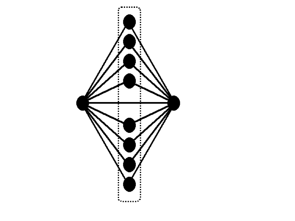
FIG. 1.: The above network is composed by $N+2$ nodes in total: $N$ nodes (the ones contained in the dotted square), plus other two nodes on the two sides. The transitivity $T$ for such network is equal to $3/(N+2)$, and therefore becomes zero in the limit of large networks. On the other hand, the clustering coefficient $C$ is $\frac{N^{2}+N+4}{N^{2}+3N+2}$, which always stays close to one.

In ref.[6] Watts and Strogatz use instead another quantity to measure the local degree of clustering. They propose to calculate the so-called clustering coefficient $C$. This quantity gives the average cliquishness of the nodes of $\bf G$, and is defined as follows. First of all a quantity $C_{i}$, the local clustering coefficient of node $i$, is defined as:

$$C_{i} = {\mbox{ \# of edges in $\bf G_{i}$ }\over\mbox{maximum possible \# of edges in $\bf G_{i}$ }}=$$ (3)

$$= {\mbox{ \# of edges in $\bf G_{i}$ }\over\mbox{ $k_{i}(k_{i}-1)/2$ }}$$ (4)

where $\bf{G_{i}}$ is the subgraph of neighbours of $i$, and $k_{i}$ is the number of neighbours of vertex $i$. Then at most $k_{i}(k_{i}-1)/2$ edges can exist in $\bf{G_{i}}$, this occurring when the subgraph $\bf{G_{i}}$ is completely connected (every neighbour of $i$ is connected to every other neighbour of $i$). $C_{i}$ denotes the fraction of these allowable edges that actually exist, and the clustering coefficient $C({\bf G})$ of graph $\bf G$ is defined as the average of $C_{i}$ over all the vertices $i$ of $\bf G$:

$$C({\bf G})=\frac{1}{N}\sum_{i\in{\bf G}}C_{i}$$ (5)

In definitive $C$ is the average cliquishness of the nodes of $\bf G$. It is important to observe that $C$, although apparently similar to $T$, is in fact a different measure. For example, consider the network in fig.1: for that network, as $N$ gets large the transitivity gets worst and worst, and $T$ approaches $0$. On the other hand, $C$ instead always stays close to $1$. Therefore, while in many occasions $C$ is indeed a good approximation of transitivity, it is in fact a totally different measure. We will see in the rest of the paper how in fact $C$ can be seen as the approximation of a different measure (efficiency).

C The small-world behavior: the WS model

The mathematical characterization of the small-world behavior proposed by Watts and Strogatz is based on the evaluation of the two quantities we have just defined: the characteristic path length $L$, measuring the typical separation between two generic nodes in the network, and the clustering coefficient $C$, measuring the average cliquishness of a node. As we will see in the following of this section, small-world networks are somehow in between regular and random networks: they are highly clustered like regular lattices, yet having small characteristics path lengths like random graphs.

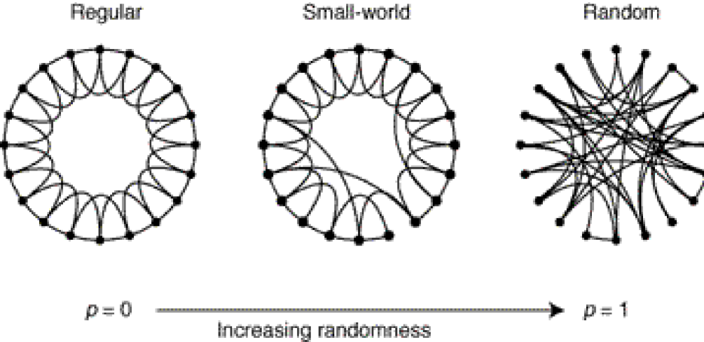
FIG. 2.: The rewiring procedure of the WS model interpolates between a regular lattice and a random graph without altering the number of nodes or edges. The regular lattice has $N=20$ nodes, each connected to its $4$ neighbours ($k=4$), and a total number of edges $K=40$. As the rewiring probability $p$ increases, the network becomes increasingly disordered. For $p=1$ a random graph is obtained. After Watts and Strogatz [6].

In ref.[6] Watts and Strogatz propose a one-parameter model (the WS model) to construct a class of graphs $\bf G$ which interpolates between a regular lattice and a random graph. The WS model is a method to produce a class of graphs with increasing randomness without altering the number of nodes or edges: an example is reported in Fig.2. The WS model starts with a one-dimensional lattice with $N$ vertices, $K$ edges, and periodic boundary conditions. Every vertex in the lattice is connected to its $k$ neighbours ($k=4$ in figure). The random rewiring procedure consists in going through each of the edges in turn and independently with some probability $p$ rewire it. Rewiring means shifting one end of the edge to a new vertex chosen randomly with a uniform probability, with the only exception as to avoid multiple edges (more than one edge connecting the same couple of nodes), self-connections (a node connected by an edge to itself), and disconnected graphs. In this way it is possible to tune $\bf G$ in a continuous manner from a regular lattice ($p=0$) into a random graph ($p=1$), without altering the average number of neighbours equal to $k=2K/N$.

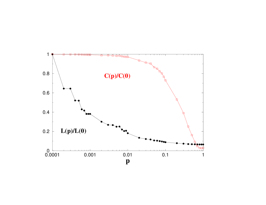
FIG. 3.: Characteristic path length $L$, and clustering coefficient $C$ for the class of graphs produced by the WS model. Here we consider $N=1000$ and $k=10$. As function of $p$ the rewiring procedure interpolates between a regular lattice ($p=0$) and a random graph ($p=1$), and produces the small-world behavior for $p$ in the range 0.01-0.1

Let us examine first the behavior of $L$ and $C$ in the two limiting cases (an analytical estimate is possible in both cases [6, 10, 28]):
— for the regular lattice ($p=0$ in the WS model), we expect $L\sim N/2k$ and a relatively high clustering coefficient $C=3/4(k-2)/(k-1)$.
— for the random graph ($p=1$ in the WS model), we expect $L\sim\ln N/ln(k-1)$ and $C\sim k/N$.
It is worth to stress how regular and random graphs behave differently when we change the size of the system $N$. If we increase $N$, keeping fixed the average number of edges per vertex $k$, we see immediately that for a regular graph $L$ increases with the size of the system, while for a random graph $L$ increases much slower, only logarithmically with $N$. On the other hand, the clustering coefficient $C$ does not depend on $N$ for a regular lattice, while it goes to zero in large random graphs. From these two limiting cases one could argue that short $L$ is always associated with small $C$, and long $L$ with large $C$. Instead social systems, which are a paradigmatic example of a small-world network, can exhibit, at the same time, short characteristic path length[8] like random graphs, and high clustering [26]. Now we can come back to the WS model. To understand the coexistence of small characteristic path length and high clustering, typical of the small-world behavior, we report in Fig.3 the behavior of $L$ and $C$ as a function of the rewiring probability $p$ for a graph with $N=1000$ and $k=10$. We follow the same lines of [6] and we normalize the two quantities by their value at $p=0$ in order to have $0\leq C(p)/C(0)\leq 1$ and $0\leq L(p)/L(0)\leq 1~{}\forall p$. Although in the two limiting cases large $C$ is associated to large $L$ and viceversa small $C$ to small $L$, the numerical experiment reveals very interesting properties in the intermediate regime: only few rewired edges (small $p\neq 0$) are sufficient to produce a rapid drop of $L$, while $C$ is not affected and remains equal to the value for the regular lattice. In this intermediate regime the network is highly clustered like regular lattices and has small characteristic path lengths like random graphs. These networks are named small worlds in analogy with the small-world phenomenon empirically observed in social systems more than 30 years ago by the social psychologist Stanley Milgram [8]. Milgram performed the first experiment to measure the length of the shortest acquaintance chain between two generic individuals in United States, and found an average length equal to 5, a value extremely small if compared to the population of the United States (about 200 millions in 1967). The WS model is a way to construct networks with the characteristics of a small-world. Of course the main question to ask now is if the small-world behavior is only a feature of an abstract model as the WS model, or if it can be present in real networks. The mathematical formalism presented can be used to analyze real systems. Watts and Strogatz have applied their mathematical formalism, based on the evaluation of $L$ and $C$ to study the topological properties of real networks databases. In their paper [6] they consider three different networks:
1) an example of social network, the collaboration graph of actors in feature films [29],
2) the neural network of a nematode, the C. elegans [30] as an example of a biological network
3) a technological network, the electric power grid of the western United States.
They show that the three networks, when considered as unweighted networks, are all examples of small worlds.

III A NEW FORMULATION VALID FOR WEIGHTED NETWORKS

Having a mathematical characterization of the small-world behavior makes it tempting to apply the same concept to any complex system. This grand plan clashes with the fact that the mathematical formalism of Watts and Strogatz suffers from severe limitations.
First of all it works only in the topological abstraction (the approximation of unweighted network), where the only information retained is about the existence or the absence of a link, and nothing is known about the physical length of the link (or more generically the weight associated to the link, see the first assumption in the original formulation of Section II where the graph G is assumed to be unweighted), and multiple edges between the same couple of nodes are not allowed (see the second assumption: G must be simple).
Moreover it applies only to some cases, whereas in general the two quantities $L$ and $C$ are ill-defined: for example the assumption number four of connectedness (see Section II) is necessary because otherwise the quantity $L$ would diverge.

The inadequacy of the Watts and Strogatz formalism is already evident to a more accurate analysis of the same three examples presented in their paper. Let us analyze the three examples one by one. In the case of films actor two are the problems: the original formalism can not be applied directly to the whole network, but it works only when the analysis is restrained to the giant connected component of the graph[6] in order to avoid the divergence of $L$. Moreover the topological approximation only provides whether actors participated in some movie together, or if they did not at all. Of course, in reality there are instead various degrees of correlation: two actors that have done ten movies together are in a much stricter relation than two actors that have acted together only once. We can better shape this different degree of friendship by using a non-simple graph or by using a weighted network: if two actors have acted together we associate a weight to their connection by saying that the length of the connection, instead of being always equal to one, is equal to the inverse of the number of movies they did together. In the case of the neural network of the C. elegans Watts and Strogatz define an edge in the graph when two vertices are connected by either a synapse or a gap junction[6]. This is only a crude approximation of the real network. Neurons are different one from the other, and some of them are in much stricter relation than others: the number of junctions connecting a couple of neurons can vary a lot, up to a maximum of 72. As in the case of film actors a weighted network is more suited to describe such a system and can be defined by setting the length of the connection $i-j$ as equal to the inverse number of junctions between $i$ and $j$. To conclude with the last example presented by Watts and Strogatz, the electrical power grid of the western United States, which is clearly a network where the geographical distances play a fundamental role. Any of the high voltage transmission lines connecting two stations of the network has a length, and the topological approximation of the Watts and Strogatz’s mathematical formalism, which neglect such lengths, is a poor description of the system. Of course a generalization of the original formalism to weighted networks would allow the study of the connectivity properties of many complex systems, extending the application of the small-world concept to a realm of new networks previously not considered. A very significative example is that of a transportation system : public transportation (bus, subway and trains), highways, airplane connections. Transportation systems can be analyzed at different levels and in this paper we will present an example of an application to urban public transportation.

The problems in the passage from abstract networks to real complex systems can be overcome by using a more general formalism, in part already presented in ref. [21], and here described in details and extended by the introduction of a new variable quantifying the cost of a network. In the following of this Section we show that:

1) A weighted network can be characterized by introducing the variable efficiency $E$, which measures how efficiently the nodes exchange information. The definition of small-world behavior can be formulated in terms of the efficiency: this single measure evaluated on a global and on a local scale plays in turn the role of $L$ and $C$. Small-world networks result as systems that are both globally and locally efficient.

2) The formalism is valid both for weighted and unweighted (topological) networks. In the case of topological networks our formalism does not coincide exactly with the one given by Watts and Strogatz. For example our formalism applies to unconnected graphs.

3) An important quantity, previously not considered is the cost of a network. Often high (global and local) efficiency implies an high cost of the network.

We are now ready to describe our new formalism. Since in general a real complex system is better described by a weighted network, we now start by considering a generic graph $\bf G$ as a weighted and possibly even non-connected and non-sparse graph. A weighted graph needs two matrices to be described:

– the adjacency matrix $\{a_{ij}\}$, containing the information about the existence or not existence of a link, and defined as for the topological graph as a set of numbers $a_{ij}=1$ when there is an edge joining $i$ to $j$, and $a_{ij}=0$ otherwise;

– a matrix of the weights associated to each link. We name this matrix $\{\ell_{ij}\}$ the matrix of physical distances because the number $\ell_{ij}$ can be imagined as the space distance between $i$ and $j$. We suppose $\ell_{ij}$ to be known even if in the graph there is no edge between $i$ and $j$. To make a few concrete examples:
$\ell_{ij}$ can be identified with the geographical distance between stations $i$ and $j$ both in the case of the electrical power grid of the western United States studied by Watts and Strogatz, and in the case of other transportation systems considered in this paper. In such a situation $\ell_{ij}$ respect the triangular inequality though in general this is not a necessary assumption.
The presence of multiple edges, typical of the neural network of the C. elegans and of social systems like the network of films actors, can be included in the same framework by setting $\ell_{ij}$ equal to the inverse number of edges between $i$ and $j$ (respectively the inverse number of junctions between two neurons, or the inverse of the number of movies two actors did together). This allows to remove the hypothesis of simple network in the (assumptions number 2 in the formalism of of Watts and Strogatz) and to consider also $\it non-simple$ systems as weighted networks. The resulting weighted network is, of course, a case in which the triangular inequality is not satisfied. For a computer network or Internet $\ell_{ij}$ can be assumed to be proportional to the time needed to exchange a unitary packet of information between $i$ to $j$ through a direct link. Or as $1/v_{ij}$, the inverse velocity of a chemical reactions along a direct connection in a metabolic network. Of course, in the particular case of an unweighted (topological) graph $\ell_{ij}=1~{}\forall i\neq j$.

A The efficiency $E$

In a weighted graph, the definition of the shortest path length $d_{ij}$ between two generic points $i$ and $j$, is slightly different than the definition used in Section II for an unweighted graph. In this case the shortest path length $d_{ij}$ is in fact defined as the smallest sum of the physical distances throughout all the possible paths in the graph from $i$ to $j$. Again, when $\ell_{ij}=1~{}\forall i\neq j$, i.e. in the particular case of an unweighted graph, $d_{ij}$ reduces to the minimum number of edges traversed to get from $i$ to $j$.
The matrix of the shortest path lengths $\{d_{ij}\}$ is therefore calculated by using the information contained both in matrix $\{a_{ij}\}$ and in matrix $\{\ell_{ij}\}$ [31]. We have $d_{ij}\geq\ell_{ij}~{}\forall i,j$, the equality being valid when there is an edge between $i$ and $j$. Let us now suppose that every vertex sends information along the network, through its edges. We assume that the efficiency $\epsilon_{ij}$ in the communication between vertex $i$ and $j$ is inversely proportional to the shortest distance: $\epsilon_{ij}=1/d_{ij}~{}\forall i,j$. Note that here we assume that efficiency and distance are inversely proportional. This is a reasonable approximation in general, and in particular for all the systems considered in this paper. Of course, sometimes other relationships might be used, especially when justified by a more specific knowledge about the system. By assuming $\epsilon_{ij}=1/d_{ij}$, when there is no path in the graph between $i$ and $j$ we get $d_{ij}=+\infty$ and consistently $\epsilon_{ij}=0$. Consequently the average efficiency of the graph $\bf G$ can be defined as [32]:

$$E({\bf G})=\frac{{{\sum_{{i\neq j\in{\bf G}}}}\epsilon_{ij}}}{N(N-1)}=\frac{1}{N(N-1)}{\sum_{{i\neq j\in{\bf G}}}\frac{1}{d_{ij}}}$$ (6)

Throughout this paper we consider undirected graphs, i.e. there is no associated direction to the links. This means that both $\{\ell_{ij}\}$ and $\{d_{ij}\}$ are symmetric matrices and therefore the quantity $E({\bf G})$ can be defined simply by using only half of the matrix as: $E({\bf G})=\frac{2}{N(N-1)}{\sum_{{i<j\in{\bf G}}}\frac{1}{d_{ij}}}$. Anyway we prefer to give the more general definition (6) since our formalism can be easily applied to directed graphs as well.

Formula (6) gives a value of $E$ that can vary in the range $[0,\infty[$. It would be more practical to have $E$ normalized to be in the interval $[0,1]$. $E$ can be normalized by considering the ideal case ${\bf{G^{ideal}}}$ in which the graph $\bf G$ has all the $N(N-1)/2$ possible edges. In such a case the information is propagated in the most efficient way since $d_{ij}=\ell_{ij}~{}\forall i,j$, and $E$ assumes its maximum value $E({\bf{G^{ideal}}})=\frac{1}{N(N-1)}{\sum_{{i\neq j\in{\bf G}}}\frac{1}{\ell_{ij}}}$. The efficiency $E({\bf G})$ considered in the following of the paper are always divided by $E({\bf{G^{ideal}}})$ and therefore $0\leq E({\bf G})\leq 1$. Though the maximum value $E=1$ is typically reached only when there is an edge between each couple of vertices, real networks can nevertheless assume high values of $E$.

B Global and local efficiency

One of the advantages of the efficiency-based formalism is that a single measure, the efficiency $E$ (instead of the two different measures $L$ and $C$ used in the WS formalism) is sufficient to define the small-world behavior.

In fact, on one side, the quantity defined in equation (6) can be evaluated as it is for the whole graph $\bf G$ to characterize the global efficiency of $\bf G$. We therefore name it $E_{\rm glob}$:

$$E_{\rm glob}=\frac{E({\bf G})}{E({\bf G^{ideal}})}$$ (7)

As said before, the normalization factor ${E({\bf G^{ideal}})}$ is the efficiency of the ideal case ${\bf{G^{ideal}}}$ in which the graph $\bf G$ has all the $N(N-1)/2$ possible edges. Being the efficiency in communication between two generic vertices, $E_{\rm glob}$ plays a role similar to the inverse of the characteristic path length $L$. In fact $L$ is the mean of $d_{ij}$, while $E_{\rm glob}$ is the average of $1/d_{ij}$, i.e. the inverse of the harmonic mean of $\{d_{ij}\}$. Nowadays the harmonic mean finds extensive applications in a variety of different fields: in particular it is used to calculate the average performance of computer systems[32, 33], parallel processors[34], and communication devices (for example modems and Ethernets[35]). In all such cases, where a mean flow-rate of information has to be computed, the simple arithmetic mean gives the wrong result. As we will see in Section (III C) and in Section (III E), in some cases $1/L$ gives a good approximation of $E_{\rm glob}$, although $E_{\rm glob}$ is the real variable to be considered when we want to characterize the efficiency of a system transporting information in parallel. In the particular case of a disconnected graph the difference between the two quantities is evident because $L=+\infty$ while $E_{\rm glob}$ is a finite number.

On the other side the same measure, the efficiency, can be evaluated for any subgraph of $\bf G$, and therefore it can be used also to characterize the local properties of the graph. In the WS formalism it is not possible to use the characteristic path length for quantifying both the global and the local properties of the graph simply because $L$ can not be calculated locally, most of the subgraphs of the neighbors of a generic vertex $i$ being disconnected. In our case, since $E$ is defined also for a disconnected graph, we can characterize the local properties of $\bf G$ by evaluating for each vertex $i$ the efficiency of $\bf{G_{i}}$, the subgraph of the neighbors of $i$. We define the local efficiency as:

$$E_{\rm loc}=1/N\sum_{i\in{\bf G}}~{}\frac{E(\bf{G_{i}})}{E(\bf{G_{i}^{ideal}})}$$ (8)

Here, for each vertex $i$, the normalization factor ${E({\bf G_{i}^{ideal}})}$ is the efficiency of the ideal case ${\bf{G_{i}^{ideal}}}$ in which the graph $\bf G_{i}$ has all the $k_{i}(k_{i}-1)/2$ possible edges. $E_{\rm loc}$ is an average of the local efficiency and plays a role similar to the clustering coefficient $C$. Since $i\notin\bf{G_{i}}$, the local efficiency $E_{\rm loc}$ tells how much the system is fault tolerant, thus how efficient is the communication between the first neighbours of $i$ when $i$ is removed. This concept of fault tolerance is different from the one adopted in Ref. [36, 37, 38], where the authors consider the response of the entire network to the removal of a node $i$. Here the response of the subgraph of first neighbours of $i$ to the removal of $i$ is considered.

We can now introduce a new, generalizing, definition of small-world, built in terms of the characteristics of information flow at global and local level: a small-world network is a network with high $E_{\rm glob}$ and $E_{\rm loc}$, i.e. very efficient both in global and local communication. This definition is valid both for unweighted and for weighted graphs, and can also be applied to disconnected graphs and/or non sparse graphs.

C Comparison between $E_{\rm glob},E_{\rm loc}$ and $L,C$

It is interesting to study more in detail the correspondence between our measure and the quantities $L$ and $C$ of [6] (or, correspondingly, $1/L$ and $C$). The fundamental difference is that $1/L$ measures the efficiency of a sequential system, that is to say, of a system where there is only one packet of information going along the network. On the other hand, $E_{\rm glob}$ measures the efficiency for parallel systems, where all the nodes in the network concurrently exchange packets of information. This can explain why $L$ works reasonably: it can be seen that $1/L$ is a reasonable approximation of $E_{\rm glob}$ when there are not huge differences among the distances in the graph, and so considering just one packet in the system is more or less equivalent to the case where multiple packets are present. This is the case for all the networks presented in [6], and this effect is strengthened even more by the fact that the topology only is considered. Having explained why $L$ behaves relatively well in some case, it is also worth noticing that, like every “approximation”, it fails to properly deal with all cases. For example, the sequentiality of the measure $1/L$ explains why many limitations have to be introduced, like connectedness, that are present just in order to make the formulas valid. Consider the limit case where a node is isolated from the system. In the case of a neural network, this corresponds for example to the death of a neuron. In this case, $1/L$ drops to zero ($L=+\infty$), which is of course not the overall efficiency of the system: in fact, the brain continues to work, as all the other neurons continue to exchange information; only, the efficiency is just slightly diminished, as now there’s one neuron less. And, correctly, this is properly taken into account using $E_{\rm glob}$. Even without dropping the connectedness assumption, another example can show how in the limit case, the approximation given by $1/L$ diverges from the real efficiency measure. Let us consider the Internet and the situation represented in Figure 4: suppose we attach a new computer to the Internet (which already had $N$ nodes), with efficiency $\varepsilon$, that can be seen as the speed of the connection. This happens every time the Internet is augmented with a new computer, and every time we turn on our computer in the office. A situation like this occurs daily in the order of the millions. How does it globally affect the Internet, according to $L$ and $E_{\rm glob}$? It can be proved that $L$ augments by approximately $\frac{1}{\varepsilon(N+1)}$. This means that if for any reason, the connection speed is particularly slow (or becomes such, for example due to a congestion, or the computer gets low in resources), the whole Internet’s $L$ is heavily affected and can rapidly become enormous. Even, whenever the computer blocks (or it’s shut down), $L$ diverges to infinity (like, so to say, if the Internet had collapsed). On the other hand, the efficiency $E_{\rm glob}$ has a relative decrement of approximately $\frac{2}{N+1}$, which means that in practice, as $N$ is quite large, the particular behaviour of the new computer affects the Internet in a negligible way. Summing up, having one or few computer with an extremely slow connection, does not mean that the whole Internet diminishes by far its efficiency: in practise, the presence of such few very slow computers goes unnoticed, because the other thousands of computers are exchanging packets among them in a very efficient way. Therefore, $L$ fails to properly capture the global behaviour of systems like the Internet ($1/L$ would give a number very close to zero because, it measures the average efficiency in case a single packet is active thorough the Internet), unlike $E_{\rm glob}$, that perfectly matches the observed behaviour.

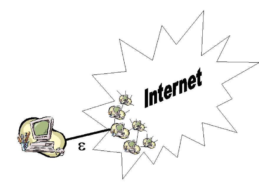
FIG. 4.: We attach a new computer to the Internet (which already had $N$ nodes), with a connection represented by a small efficiency $\varepsilon$. Having one (or few) computer with an extremely slow connection, does not mean that the whole Internet diminishes by far its efficiency: in practise, the presence of such slow computer goes unnoticed, because the other thousands of computers are exchanging packets among them in a very efficient way. $L$ fails to properly capture the global behaviour of systems like the Internet, unlike $E_{\rm glob}$, that perfectly matches the observed behaviour (see text).

The crucial point here is the following: all the networks considered in [6] to justify the definition of small-worlds (and, in fact, most of the networks the model complex systems) are parallel systems, where all the nodes interact in parallel (Internet, World Wide Web, social networks, neural systems and so on). With this assumption, $E_{\rm glob}$ measures the real efficiency of the system, and $1/L$ is just a first rough approximation, as it deals with the sequential case only.

We turn now our attention to $C$ and $E_{\rm loc}$. As we have seen in Section II, the true meaning of the clustering coefficient $C$ cannot be sought in the classic clustering measure of social sciences, i.e. transitivity: the two quantities may diverge, giving diametrically opposite results for the same networks. On the other hand, it can be shown that $C$, in the case of undirected topological graphs, is always a reasonable approximation of $E_{\rm loc}$. Therefore, the seemingly ad-hoc nature of $C$ in the WS formalism, now finds a new meaning in the general notion of efficiency: there are not two different kinds of properties to consider when analyzing a network on the local and on the global scale, but just one unifying concept: the efficiency to transport information.

D The Cost of a Network

An important variable to consider, especially when we deal with weighted networks and when we want to analyze and compare different real systems, is the cost of a network. In fact, we expect the efficiency of a graph to be higher as the number of edges in the graph increases. As a counterpart, in any real network there is a price to pay for number and length (weight) of edges. In particular the ’short cuts’, i.e. the rewired edges that produce the rapid drop of $L$ and the onset of the small-world behavior in the WS model connect at no cost vertices that would otherwise be much farther apart. It is therefore crucial to consider weighted networks and to define a variable to quantify the cost of a network. In order to do so, we define the cost of the graph $\bf G$ as:

$$Cost({\bf G})=\frac{\sum_{{i\neq j\in{\bf G}}}a_{ij}\gamma(\ell_{ij})}{\sum_{{i\neq j\in{\bf G}}}{\gamma(\ell_{ij})}}$$ (9)

Here, $\gamma$ is the so-called cost evaluator function, which calculates the cost needed to build up a connection with a given length. Of course, $\gamma$ could be equivalently defined on efficiencies rather than distances (so, indicating in a sense the cost to set up a communication channel with the given efficiency). Note that we have already included in the numerator of this definition the cost of ${\bf G}^{ideal}$, the ideal graph in which all the possible edges are present. Because of such a normalization, the $\gamma$ function needs only to be defined up to a multiplicative constant, and the quantity $Cost({\bf G})$ is defined in the interval $[0,1]$, assuming the maximum value $1$ for ${\bf G}^{ideal}$, i.e. when all the edges are present in the graph. $Cost({\bf G})$ reduces to the normalized number of edges $2K/N(N-1)$ in the case of an unweighted graph (for example the WS model).
Unless otherwise specified, we will assume in the following that $\gamma$ is defined as the identity function: $\gamma(x)=x$. In fact such a cost evaluator works for unweighted networks, and also for most of the real networks, those where the cost of a connection is proportional to its length (to the euclidean distance for example): in all such cases the definition of the cost reduces to $Cost({\bf G})=({\sum_{{i\neq j\in{\bf G}}}a_{ij}\ell_{ij}})/({\sum_{{i\neq j\in{\bf G}}}{\ell_{ij}}})$. A different definition of the cost evaluator function will be used instead when we represent networks with multiple edges as weighted graphs (for examples in the weighted C. elegans and in the weighted movie actors).

With our formalism based on the two efficiencies $E_{\rm glob}$ and $E_{\rm loc}$, and on the variable $Cost$, all defined in the range from $0$ to $1$, we can study in an unified way unweighted (topological) and weighted networks. We therefore define the following key notion: let us call economic every network with low $Cost$; then, an economic small-world is a network having high $E_{\rm loc}$ and $E_{\rm glob}$, and low $Cost$ (i.e., both economic and small-world).

E The economic small-world behavior

We are now ready to illustrate the three quantities $E_{\rm glob}$, $E_{\rm loc}$ and $Cost$ at work in some practical examples. Starting from the original WS model, and proceeding with different models, we will illustrate how these three quantities behave in a dynamic environment where the network changes, have some nontrivial interaction among each other, and give birth to small-worlds [24, 31]. Model 1 (the WS model) is a procedure to construct a family of unweighted networks with a fixed cost. Model 2 is a way to construct unweighted networks, this time with increasing cost. Model 3 and model 4 are two examples of weighted networks. In particular in model 4 the length of the edge connecting two nodes is the euclidean distance between the nodes.

Model 1) The original WS model is unweighted (topological): this means we can set $\ell_{ij}=1~{}\forall i\neq j$, and the quantities $d_{ij}$ reduce to the minimum number of edges to get from $i$ to $j$. The dynamic changes of the network consist in rewirings: since the weight is the same for all edges, also for rewired edges, this means that the $Cost$ (that is proportional to the total number of edges $K$) does not change with the rewiring probability $p$. In fig.5 we consider a regular lattice with $N=1000$ and three different values of $k$ ($k=6,10,20$), corresponding to networks with different (low) cost (respectively $Cost=0.006,0.01,0.02$), and we report $E_{\rm glob}$ and $E_{\rm loc}$ as a function of $p$ [24]. For $p=0$ we expect the system to be inefficient on a global scale (an analytical estimate gives $E_{\rm glob}\sim k/N~{}log(N/K)$), but locally efficient. The situation is inverted for random graphs. In fact, for example in the case $k=20$, at $p=1$ $E_{\rm glob}$ assumes a maximum value of $0.4$, meaning $40\%$ the efficiency of the ideal graph with an edge between each couple of vertices. This happens at the expenses of the fault tolerance ($E_{\rm loc}\sim 0$). The (economic) small-world behavior appears for intermediate values of $p$. It results from the fast increase of $E_{\rm glob}$ caused by the introduction of only a few rewired edges (short cuts), which on the other side do not affect $E_{\rm loc}$. For the case $k=20$, at $p\sim 0.1$, $E_{\rm glob}$ has almost reached the maximum value of $0.4$, though $E_{\rm loc}$ has only diminished by very little from the maximum value of $0.82$. For such an unweighted case the description in terms of network efficiency is similar to the one given by Watts and Strogatz. In fig.6 we show that if we report the quantities $1/E_{\rm glob}(p)$ and $E_{\rm loc}(p)$, and we use a normalization similar to the one adopted by Watts and Strogatz, i.e. $E_{\rm glob}(0)/E_{\rm glob}(p)$ and $E_{\rm loc}(p)/E_{\rm loc}(0)$, we get curves with qualitatively the same behavior of the curves $L(p)/L(0)$ and $C(p)/C(0)$ (compare with fig.3).

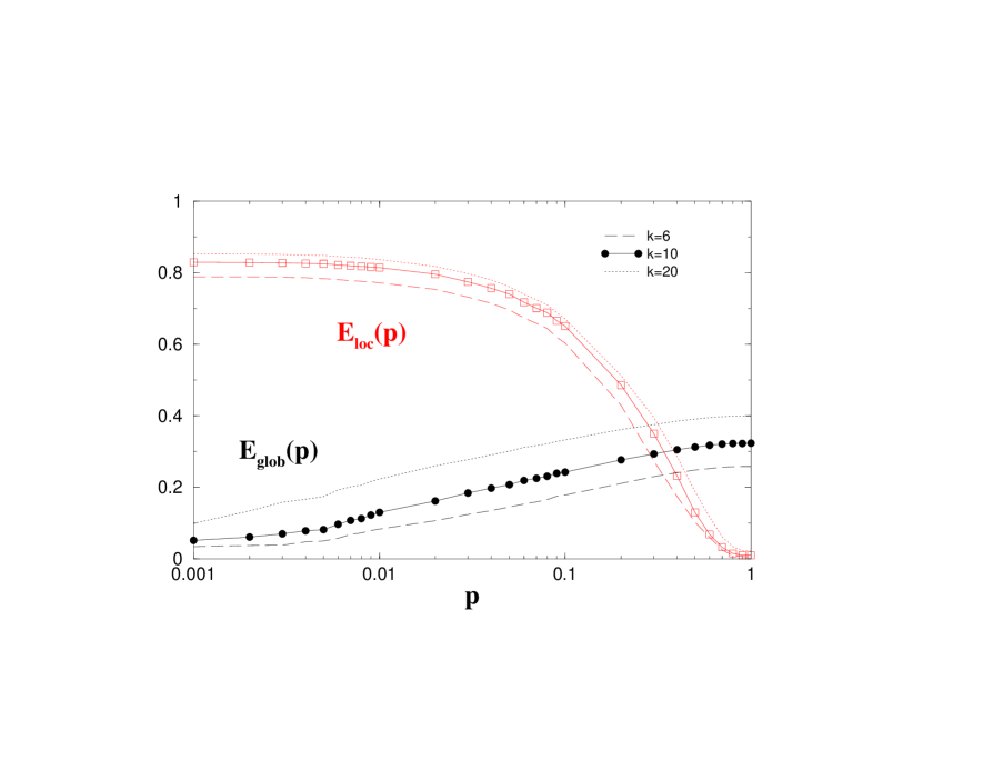
FIG. 5.: Global and local efficiency for model 1 (the WS model), the class of topological graphs considered by Watts and Strogatz. A regular lattice with $N=1000$ and $k$ edges per node is rewired with probability $p$. The logarithmic horizontal scale is used to resolve the rapid increase in $E_{\rm glob}$ due to the presence of short cuts and corresponding to the onset of the small-world. During this increase, $E_{\rm loc}$ remains large and almost equal to the value for the regular lattice. Small worlds have high $E_{\rm glob}$ and $E_{\rm loc}$. We consider three different values $k=6,10,20$ corresponding respectively to $Cost=0.006,0.01,0.02$.

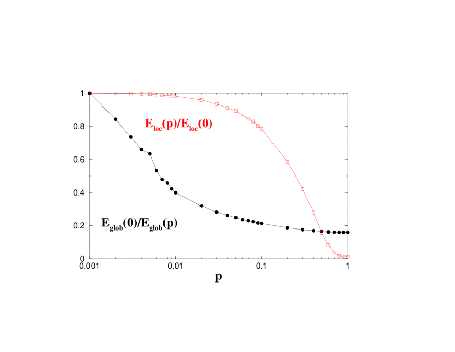
FIG. 6.: Model 1 (the WS model). A regular lattice with $N=1000$ and $k=10$ edges per node is rewired with probability $p$. Reporting the quantities $\left(\frac{E_{\rm glob}(p)}{E_{\rm glob}(0)}\right)^{-1}$ and $\frac{E_{\rm loc}(p)}{E_{\rm loc}(0)}$ as a function of $p$, the two curves show a behavior similar respectively to $L(p)$ and $C(p)$.

Model 2) The above model has proved successful in order to produce small-worlds, i.e. networks with high $E_{\rm glob}$ and high $E_{\rm loc}$. However, if that is the goal, then there are much simpler procedures that can output a small world, even starting from an arbitrary configuration. For example in Fig.7 we consider a model where, starting from a configuration with $N=100$ nodes and no links we keep adding links randomly, until we reach a completely connected network. This model is unweighted as model 1. Contrarily to the case of model 1, the network changes by adding links, then the cost is not a fixed quantity but varies in a monotonic way, increasing every time we add a link. As we can see, for $Cost\sim 0.5-0.6$ we obtain a small-world network with $E_{\rm glob}=E_{\rm loc}=0.8$. So, if this trivial method manages to produce small worlds, why can’t we find many small worlds like these in nature ? The obvious answer is that here, we are obtaining a small-world at the expense of the cost: with rich resources (high cost), the small-world behaviour always appears. In fact, in the limit of the completely connected network ($Cost=1$) we have $E_{\rm glob}=E_{\rm loc}=1$. But what also matters in nature is also economy of a network, and in fact a trivial technique like this fails to produce economic small worlds.
Note also that the relationship of the variable cost with respect to the other two variables is not that trivial. Even in the very simple and rigid ”monotonic” setting dictated by this model we observe an interesting behavior of the variables $E_{\rm glob}$ and $E_{\rm loc}$ as functions of $Cost$. In particular we observe a rapid rise of $E_{\rm loc}$ when the cost increases from $0.1$ to $0.2$. This means that moving from $Cost=0.1$ to $Cost=0.2$ we can increase the local efficiency of the network from $E_{\rm loc}=0.1$ to $E_{\rm loc}=0.6$. We therefore obtain a network with $60\%$ of the efficiency of the ideal network both on a global and local scale, with only the $20\%$ of the cost: this is an example of an economic small-world network. The effect we have observed has an higher probability to happen in the mid-area inbetween the areas of low cost and high cost, and it is a first sign that complex interactions do occur, but not with very low cost or with very high cost (where economic small-worlds can’t be found).

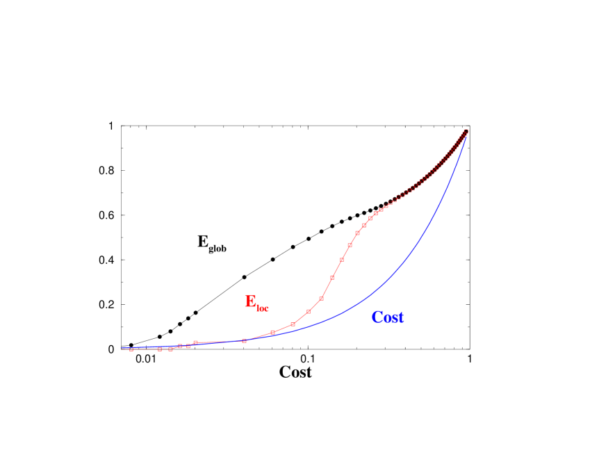
FIG. 7.: Model 2. A network is created by adding links randomly to an initial configuration with $N=100$ nodes and no links. $E_{\rm glob}$ and $E_{\rm loc}$ are plotted as functions of the $Cost$. The identity curve $Cost$ is also reported to help the reader since a logarithmic horizontal scale is used.

Model 3) In this third model, we combine features of the previous models 1 and 2: we adopt rewiring as in model 1, monotonic increase of the cost as in model 2. So, while in model 1 the short cuts connect at no cost (because $\ell_{ij}=1~{}\forall i\neq j$) vertices that would otherwise be much farther apart (which is a rather unrealistic assumption for real networks), in this model each rewiring has a cost. In fig.8 we implement a random rewiring in which the length of each rewired edge is set to change from 1 to 3. So, note that this model, unlike the previous two, is weighted. The figure shows that the small-world behaviour is still present even when the length of the rewired edges is larger than the original one. For $p$ around the value $0.1$ we observe that $E_{\rm glob}$ has almost reached the maximum value $0.18$ ($18\%$ of the global efficiency of the ideal graph with all couples of nodes directly connected with edges of length equal to $1$) while $E_{\rm loc}$ has not changed too much from the maximum value $0.8$ (assumed at $p=0$). The only difference with respect to model 1 is that the behaviour of $E_{\rm glob}$ is not simply monotonic increasing. Of course in this model the variable $Cost$ increases with $p$. It is interesting to notice that the curve $Cost$ as a function of $p$, plotted in the bottom of the figure, is specular to the curve $E_{\rm loc}$ as a function of $p$. This means that in the small-world situation, the network is also economic, in fact the $Cost$ stays very close to the minimum possible value (assumed of course in the regular case $p=0$). We have checked the robustness of the results obtained by increasing even more the length of the rewired edges.
Therefore, this model shows that to some extent, the structure of a network plays a relevant role in the economy. Also, note that in this more complex (weighted) model, behaviour of $E_{\rm loc}$ and $E_{\rm glob}$ become more complex as well: now, $E_{\rm glob}$ is not a monotonic function of the cost any more, and $E_{\rm loc}$ is monotonic, but decreasing. So, introduction of the weighted model further shows how the relative behaviour of the three variables $E_{\rm glob}$, $E_{\rm loc}$ and $Cost$ is far from simple.

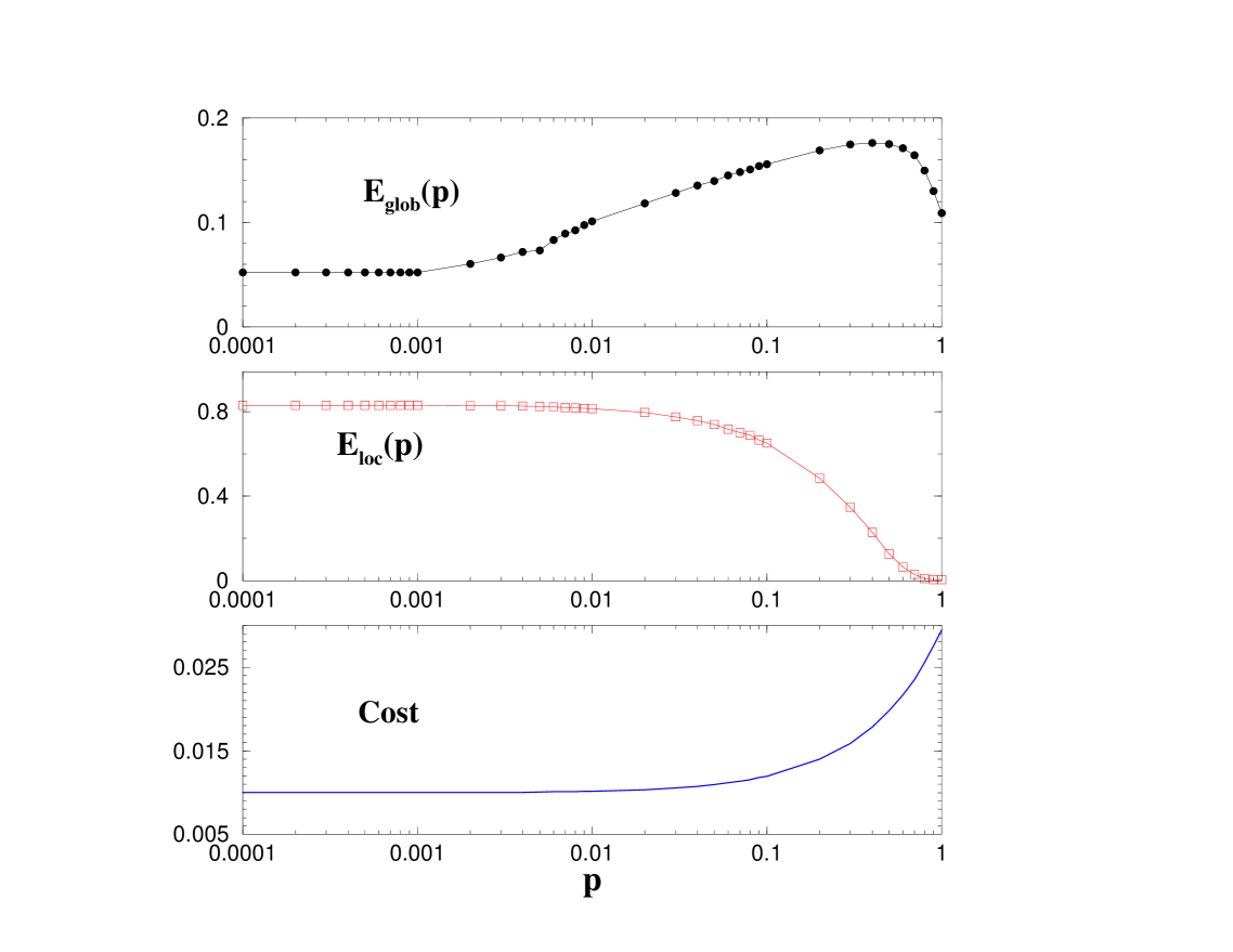
FIG. 8.: The three quantities $E_{\rm glob}$, $E_{\rm loc}$ and $Cost$ are reported as functions of $p$ in model 3. We start with a regular lattice with $N=1000$ and $k=10$ and we implement the same rewiring procedure as in the WS model, with only difference that the length of the rewired edge is set to change from the value 1 to the value 3. The economic small-world behavior shows up for $p\sim 0.1$

Model 4) As a final example we build on model 3, and ground it more in reality using a real geometry, in order to investigate further whether the above effects can also appear in real networks which are not just mathematical possibilities. In this weighted model, the length of the edge connecting two nodes is the euclidean distance between the nodes. The nodes can be placed with different geometries. Here we consider the case in which the $N$ nodes are placed on a circle as in fig.2. Now the geometry is important because the physical distance between node $i$ and $j$ ($i,j=1,...,N$) is defined as the euclidean distance between $i$ and $j$. In the case of nodes on a circle we have:

$$\ell_{ij}=\frac{2\sin(|i-j|\pi/N)}{2\sin(\pi/N)}$$ (10)

In this formula we have set the length of the arc between two neighbours to be equal to $1$, i.e. $\ell_{ij}=1$ when $|i-j|=1$. The radius of the circle is then $R=\frac{1}{2}\sin(\pi/2)/\sin(\pi/N)$. In fig.9 we report the results obtained by implementing a rewiring procedure similar to the one considered in the previous models. The only difference with respect to the previous case is that now we cannot start from a lattice with $N=1000$, $k=10$. Such a network, in fact, when considered with the metrics in formula (10) would have $K=5000$ edges and a too high global efficiency, about $99\%$ of the ideal graph. On the other side, considering as a starting network a lattice with $k=2$ would affect the local efficiency. Then we proceed as follows. We create a regular network with $N=1000$ and $k=6$ and then we eliminate randomly the $50\%$ of the $3000$ edges to decrease the global efficiency: in the random realization reported in figure we are left with $K=1507$ edges. At this point we can implement the usual rewiring process on this network. For $p\sim 0.02-0.04$ we observe that $E_{\rm glob}$ has almost reached its maximum value $0.62$ while $E_{\rm loc}$ has not changed much from the maximum value $0.2$ (assumed at $p=0$). As in model 3 the behaviour of $E_{\rm glob}$ is not simply monotonic decreasing, and as in model 3 the small-world network is also an economic network, i.e. the $Cost$ stays very close to the minimum possible value (assumed of course for $p=0$).

So, this model and model 3 suggest that the economic small-world behavior is not only an effect of the topological abstraction but can also be found in all the weighted networks where the physical distance is important and the rewiring has a cost (and, shows how intricate the relative behaviour of $E_{\rm glob}$, $E_{\rm loc}$ and $Cost$ can be).

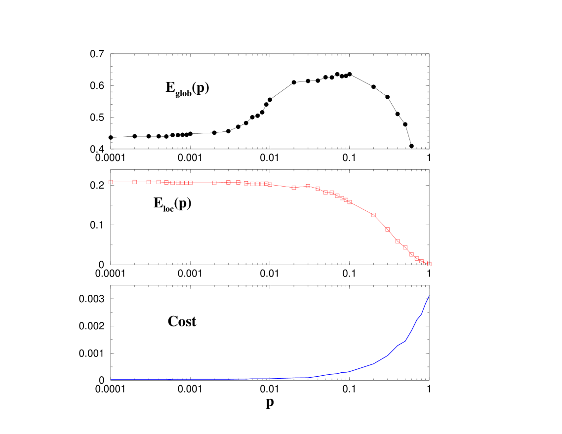
FIG. 9.: The three quantities $E_{\rm glob}$, $E_{\rm loc}$ and $Cost$ are reported as functions of $p$ in model 4. We start with a regular lattice with $N=1000$ and a total number of edges $K=1507$ (see detail in the text) and we implement the rewiring procedure with probability $p$. The economic small-world behavior shows up for $p\sim 0.02-0.04$

IV APPLICATIONS TO REAL NETWORKS

With our formalism based on the three quantities $E_{\rm glob}$, $E_{\rm loc}$, and $Cost$, all defined in the range from $0$ to $1$, we can study in an unified way unweighted (topological) and weighted networks, and we are therefore well equipped to consider some empirical examples. In this paper we present a study of 1) neural networks (two examples of networks of cortico-cortical connections, and an example of a nervous system at the level of connections between neurons), 2) social networks (the collaboration network of movie actors), 3) communication networks (the World Wide Web and the Internet), 4) transportation systems (the Boston urban transportation systems).

A Neural Networks

The brain is the most complex and fascinating information transportation system. Its staggering complexity is the evolutionary result of adaptivity, functionality and economy. The brain complexity is already reflected in the complexity of its structure [39]. Of course neural structures can be studied at several levels of scale. In fact, thanks to recent experiments, a wealth of neuroanatomical data ranging from the fine structure of connectivity between single neurons to pathways linking different areas of the cerebral cortex is now available. Here we focus first on the analysis of the neuroanatomical structure of cerebral cortex, and then on a simple nervous system at the level of wiring between neurons.
1) Networks of Cortico-cortical connections. The anatomical connections between cortical areas and group of cortical neurons are of particular importance because they are considered to have an intricate relationship with the functional connectivity of the cerebral cortex [40]. We analyze two databases of cortico-cortical connections in the macaque and in the cat [41]. The databases consist of the wiring diagrams of the two system, and there is no information about the weight associated to the links: therefore we will study these systems as unweighted networks. The macaque database contains $N=69$ cortical areas and $K=413$ connections (see ref.[42], cortical parcellation after [43], except auditory areas which follow ref. [44]). The cat database has instead $N=55$ cortical areas (including hippocampus, amygdala, entorhinal cortex and subiculum) and $K=564$ (revised database and cortical parcellation from [45]). The results in the first two lines of table I indicates the two networks are economic small-worlds: they have high global efficiency (respectively $52\%$ and $69\%$ the efficiency of the ideal graph) and high local efficiency ($70\%$ and $83\%$ the ideal graph), i.e. high fault tolerance  [46] with only $18\%$ and $38\%$ of the wirings. Moreover $E_{\rm glob}$ is similar to the value for random graphs, while $E_{\rm loc}$ is larger than $E_{\rm loc}^{random}$. These results indicate that in neural cortex each region is intermingled with the others and has grown following a perfect balance between cost, local necessities (fault tolerance) and wide-scope interactions.
2) A network of connections between neurons. As a second example we consider the neural network of C. elegans the only case of a nervous system completely mapped at the level of neurons and chemical synapses [47]. The database we have considered, is the same considered by Watts and Strogatz and is taken from ref.[30].

TABLE I.: The macaque and cat cortico-cortical connections [41] are two unweighted networks with respectively $N=69$ and $N=55$ nodes, $K=413$ and $K=564$ connections. Global efficiency, local efficiency and cost are reported in the first two lines of the table. The results are compared to the efficiency of random graphs. The nervous system of C. elegans is better described by a weighted network: the network consists of $N=282$ nodes and $K=2462$ edges which can be of two different kind, either synaptic connections or gap junctions. This time, associated to each link, there is weight (see text). In the third line of the table we report the result for the C. elegans considered as unweighted (to compare with cortico-cortical networks), while in the fourth line we consider the weights. All these systems are examples of economic small worlds.

Unweighted:	$E_{\rm glob}$	$E_{\rm glob}^{\rm random}$	$E_{\rm loc}$	$E_{\rm loc}^{\rm random}$	$Cost~{}~{}$
Macaque	0.52	0.57	0.70	0.35	0.18
Cat	0.69	0.69	0.83	0.67	0.38
C. elegans	0.46	0.48	0.47	0.12	0.06

Weighted:	$E_{\rm glob}$	$E_{\rm loc}$	$Cost~{}~{}$
C. elegans	0.35	0.34	0.18

As already discussed in Sect.III, the nervous system of C. elegans is better described by a weighted network. In fact the C. elegans is a multiple edges system, i.e. there can be more than one edge (up to $72$ edges) between the same couple of nodes $i$ and $j$. The presence of multiple edges can be expressed in our weighted networks formalism by considering a simple but weighted graph, and setting $\ell_{ij}$ equal to the inverse number of edges between $i$ and $j$. In this way we get a weighted network consisting of $N=282$ nodes and $K=2462$ edges (an edge $i-j$ is defined by the presence of at least one synaptic connection or gap junction). Now, observe that doing this choice to weight the system, we then have to define appropriately the cost evaluator function $\gamma$ (which can not be the identity any more): the correct choice is to set $\gamma(x)=1/x$, that is to say, the cost of a connection is the number of synaptic connections and gap junctions that make it.
In order to compare the C. elegans to the two cortico-cortical connections networks, we first consider it as an unweighted network neglecting the information contained in $\{\ell_{ij}\}$ (as if $\ell_{ij}=1~{}\forall i\neq j$). Similarly to the two cortico-cortical connections networks, the unweighted C. elegans is also an economic small-world network. In third line of table I we see that with a relative low cost ($6\%$ of the wirings), C. elegans achieves about a $50\%$ of both the global and local efficiency of the ideal graph (see also the comparison with the random graph). Moreover the value of $E_{\rm glob}$ is similar to $E_{\rm loc}$. This is a difference from cortex databases, where fault tolerance is slightly privileged with respect to global communication. Finally we can consider the C. elegans in all its completeness, i.e. as a weighted graph. Of course in this case the random graph does not give any more the best approximation for $E_{\rm glob}$. Nevertheless the values of $E_{\rm glob}$, $E_{\rm loc}$ and $Cost$ have a meaning by themselves, being normalized to the case of the ideal graph. We get (see the fourth line of I) that the C. elegans is also an economic small-world when considered as a weighted network with about $35\%$ of the global and local efficiency of the ideal graph, obtained with a cost of $18\%$. It is interesting to notice that, as in the unweighted case, the system has similar values of $E_{\rm glob}$ and $E_{\rm loc}$ (that is, it behaves globally in the same way as it behaves locally).
The connectivity structure of the three neural networks studied reflects a long evolutionary process driven by the need to maximize global efficiency and to develop a robust response to defect failure (fault tolerance). All this at a relatively low cost, i.e. with a small number of edges, or with a minimum amount of the length of the wirings.

B Social Networks

As an example of social networks we study the collaboration network of movie actors extracted from the Internet Movie Database[29], as of July 1999. The graph considered has $N=277336$ and $K=8721428$, and is not a connected graph. The approach of Watts and Strogatz cannot be applied directly and they have to restrict their analysis to the giant connected component of the graph[6]. Here we apply our small-world analysis directly to the whole graph, without any restriction. Moreover the unweighted case only provides whether actors participated in some movie together, or if they did not at all. Of course, in reality there are instead various degrees of correlation: two actors that have done ten movies together are in a much stricter relation rather than two actors that have acted together only once. As in the case of C. elegans we can better shape this different degree of friendship by using a weighted network: we set the distance $\ell_{i,j}$ between two actors $i$ and $j$ as the inverse of the number of movies they did together.

As in the case of the C. elegans, together with this choice to weight the system, we also have to define appropriately the cost evaluator function $\gamma$: the correct choice is (again) to set $\gamma(x)=1/x$, that is to say, the cost of a connection between two persons is the number of movies they did together.

The numerical values in table II indicate that both the unweighted and the weighted network shows the economic small-world phenomenon. In both cases, cost comes out as a leading principle: this is due somehow to physical limitations, as it is not easy for actors to perform in a huge number of movies, and for most of them, their career is in any case limited in time, while the database spans all the temporal age.

TABLE II.: The collaboration network of movie actors (extracted from the Internet Movie Database, IMD) can be described by an unweighted or a weighted graph with $N=277336$ and $K=8721428$.

Unweighted:	$E_{\rm glob}$	$E_{\rm glob}^{\rm random}$	$E_{\rm loc}$	$E_{\rm loc}^{\rm random}$	$Cost~{}~{}$
Movie Actors	0.37	0.41	0.67	0.00026	0.0002

Weighted:	$E_{\rm glob}$	$E_{\rm loc}$	$Cost~{}~{}$
Movie Actors	0.29	0.52	0.0005

Of course other social systems can be studied by means of our formalism: for example the collaboration network of physicists [16, 17], the collaboration network of Marvel comics characters [48], or some other databases of social communities [18, 49].

C Communication Networks

Communication networks are ubiquitous nowadays: the so-called ”information society” heavily relies on such networks to rapidly exchange information in a distributed fashion, all over the world. Here, we consider the two most important large-scale communication networks present nowadays: the World Wide Web and the Internet. Note that despite these two networks are often confused and identified, they are fundamentally different: the World Wide Web (WWW) network is based on information abstraction, via the fundamental concept of URI (Uniform Resource Identifier); so, it is not a physical structure, but an abstract structure. On the other hand, the Internet is a physical communication network, where each link and node have a physical representation in space. So, despite these two communication networks share lot of commonalities (last but not least, the fact the WWW essentially relies on the Internet structure to work), they are bottom-down deeply different: one network (WWW) is purely conceptual, the other one (the Internet) is physical.

TABLE III.:     Communication networks. Data on the World Wide Web from http://www.nd.edu/~networks contains $N=325729$ documents and $K=1090108$ links [19], while the Internet database is taken from http://moat.nlanr.net and has $N=6474$ nodes and $K=12572$ links. Both systems are studied as unweighted graphs and are examples of economic small worlds.

	$E_{\rm glob}$	$E_{\rm glob}^{\rm random}$	$E_{\rm loc}$	$E_{\rm loc}^{\rm random}$	$Cost~{}~{}$
WWW	0.28	0.28	0.36	0.000001	0.00002
Internet	0.29	0.30	0.26	0.0005	0.006

We have studied a database of the World Wide Web with $N=325729$ documents and $K=1090108$ links, and a network of Internet with $N=6474$ nodes and $K=12572$ links. Both networks are considered as unweighted graphs. In table III we report the result of the efficiency-cost analysis of the two networks. As we can see, they have relatively high values of $E_{\rm glob}$ (slightly smaller than the best possible values obtained for random graphs) and $E_{\rm loc}$, together with a very small cost: therefore, both of them are economic small-worlds. Observe that interestingly, despite the WWW is a virtual network and the Internet is a physical network, at a global scale they transport information essentially in the same way (as their $E_{\rm glob}$’s are almost equal). At a local scale, the larger $E_{\rm loc}$ in the WWW case can be explained both by the tendency in the WWW to create Web communities (where pages talking about the same subject tend to link to each other), and by the fact that many pages within the same site are often quickly connected to each other by some root or menu page. As far as the cost is concerned, it is striking to notice how economic these networks are (for example, compare these data with the corresponding ones for the cases of neural networks). This clearly indicates that economy is a fundamental construction principle of the Internet and of the WWW.

D Transportation Networks

We focus now on another example of man-made networks, the transportation networks. As a paradigmatic example of a system belonging to this class we consider the Boston public transportation system. Other examples, like the Paris subway systems and the network of airplanes and highway connections throughout the world, are currently under study and will be presented in a future work [50].
The Boston subway transportation system (MBTA) reported in fig.10 is the oldest subway system in the U.S. (the first electric streetcar line in Boston, which is now part of the MBTA Green Line, began operation on January 1, 1889) and consists of $N=124$ stations and $K=124$ tunnels (connecting couples of stations) extending throughout Boston and the other cities of the Massachusetts Bay [51]. As some of the previous databases, this is another example of a network better described by a weighted graph: in this case the matrix $\{\ell_{ij}\}$ is given by the euclidean distance between $i$ and $j$, i.e. by the geographical distances between stations. In this sense the MBTA is a weighted network more similar to the electrical power grid of the western United States than to weighted networks representing multiple edges systems like the neural network of the C. elegans or to the network of films actors. In fact in the case of the MBTA the quantities $\ell_{ij}$ respect the triangle inequality and the definition of the ideal graph is straightforward since the spatial distance $\ell_{ij}$ between stations $i$ and $j$ is perfectly defined, independently from the existence or not of the edge $i-j$. In particular the matrix $\{\ell_{ij}\}$ has been calculated by using information databases from the MBTA [51], from the Geographic Data Technology (GDT), and the U.S. National Mapping Division.

FIG. 10.: The Boston subway transportation system (MBTA) consists of four different lines (Green, Red, Blue and Orange), $N=124$ stations and $K=124$ tunnels extending throughout Boston and the other cities of the Massachusetts Bay [51].

The MBTA, even when considered as an unweighted network, is a typical example of a case where the WS formalism fails to apply. We therefore proceed step by step: we first study the system in the unweighted approximation (illustrating that the WS formalism based on $L$ and $C$ does not work, and must be replaced by the efficiency-based formalism). We finally represent and study the efficiency of the MBTA in its completeness, as a weighted network [21, 52].
Let us start by showing that even in the approximation of unweighted network the case of MBTA cannot be considered by the original formalism, and the efficiency-based formalism must be used. In the unweighted network approximation the information contained in $\{\ell_{ij}\}$ is not used (as if $\ell_{ij}=1~{}\forall i\neq j$). Now, consider for example $L$: if we apply to the MBTA the original formalism presented in Sect. II, valid for unweighted (topological) networks, we obtain $L=15.55$ (an average of 15 steps, or 15 stations to connect 2 generic stations). And now, to decide if the MBTA is a small world we have to compare the obtained $L$ to the respective values for a random graph with the same $N$ and $K$. But, when we consider a random graph we get $L=\infty$. So, we are unable to draw any conclusion.
On the other side, the same unweighted network can be perfectly studied by using the efficiency formalism of Sect. III. The problem of the divergence we had for $L$ is here avoided, because when there is no path in the graph between $i$ and $j$, $d_{i,j}=+\infty$ and consistently $\epsilon_{ij}=0$. The results are reported in the first line of table IV and compared with the values obtained for the random graph with same number of $N$ and $K$ (as said before, in the unweighted case, the random graph provides the best value of $E_{\rm glob}$). We see immediately that the unweighted network is not a small world because the $E_{\rm loc}$ should be much larger than $E_{\rm loc}^{\rm random}$, and is instead smaller than $E_{\rm loc}^{\rm random}$.

TABLE IV.:     The MBTA can be considered as a network of $N=124$ nodes and $K=124$ links. The MBTA is first studied as an unweighted network and then as a weighted network. Finally the weighted network consisting in the underground transportation system plus the bus transportation system is considered as a more complete transportation system. The matrix $\{\ell_{ij}\}$ has been calculated by using databases from the MBTA [51] and the U.S. National Mapping Division.

Unweighted:	$E_{\rm glob}$	$E_{\rm glob}^{\rm random}$	$E_{\rm loc}$	$E_{\rm loc}^{\rm random}$	$Cost~{}~{}$
MBTA	0.10	0.14	0.006	0.015	0.016

Weighted:	$E_{\rm glob}$	$E_{\rm loc}$	$Cost~{}~{}$
MBTA	0.63	0.03	0.002
MBTA + bus	0.72	0.46	0.004

In the second line of table IV we report the results for the weighted case, i.e. the case in which the link characteristics (lengths in this case) are properly taken into account, and not flattened into their topological abstraction. As a main difference from the unweighted case considered before, in a weighted case the random graph does not give the estimate of the highest global efficiency. In any case the quantities $E_{\rm glob}$ and $E_{\rm loc}$ have a meaning by themselves because of the adopted normalization: the numbers shows MBTA is a very efficient transportation system on a global scale but not at the local level. In fact $E_{\rm glob}=0.63$ means that MBTA is only $37\%$ less efficient than the ideal subway with a direct tunnel from each station to the others. On the other hand $E_{\rm loc}=0.03$ indicates a poor local efficiency: differently from a neural network or from a social system the MBTA is not fault tolerant and a damage in a station will dramatically affect the efficiency in the connection between the previous and the next station. To understand better the difference with respect to the other systems previously considered we need to make few general considerations about the variable $Cost$ and the rationales in the construction principles. As said before in general the efficiency of a graph increases with the number of edges. As a counterpart, in any real network there is a price to pay for number and length (weight) of edges. If we calculate the cost of the weighted MBTA we get $\it{Cost}=0.002$, a value much smaller than the ones obtained for example for the three neural networks considered, respectively $\it{Cost}=0.18,0.38,0.06-0.07$. This means that MBTA achieves the $63\%$ of the efficiency of the ideal subway with a cost of only the $0.2\%$. The price to pay for such low-cost high global efficiency is the lack of fault tolerance. The difference with respect to neural networks comes from different needs and priorities in the construction and evolution mechanism. A neural network is the results of perfect balance between global and local efficiency. On the other side, when we build a subway system, the priority is given to the achievement of global efficiency at a relatively low cost, and not to fault tolerance. In fact a temporary problem in a station can be solved in an economic way by other means: for example, waling, or taking a bus from the previous to the next station. That is to say, the MBTA is not a closed system: it can be considered, after all, as a subgraph of a wider transportation network. This property is very often so understood that it isn’t even noted (consider for example, the case of the brains), but it is nevertheless of fundamental importance when we analyze a system: while global efficiency is without doubt the major characteristic, it is closure that somehow leads a system to have high local efficiency (without alternatives, there should be high fault-tolerance). The MBTA is not a closed system, and thus this explains why, unlike in the case of neural networks fault tolerance is not a critical issue. Changing the MBTA network to take into account, for example the bus system, indeed, this extended transportation system comes back to be an economic small-world network. In fact the numbers in the third line of table IV indicate that the extended transportation system achieve high global but also high local efficiency ($E_{\rm glob}=0.72$, $E_{\rm loc}=0.43$), at a still low price ($Cost$ has only increased from $0.002$ to $0.004$). Qualitatively similar results have been obtained for other underground systems [50]. Transportation systems can of course also be analyzed at different scales: a similar analysis on a wider transportation system, consisting of all the main airplane and highway connections throughout the world, shows a small-world behavior [50]. This can be explained by the fact that in such a system we consider almost all the reasonable transportation alternatives available at that scale. In this way the system is closed, i.e. there are no other reasonable routing alternatives, and so fault-tolerance comes back, after the cost, as a leading construction principle.

V CONCLUSIONS

The small-world concept has shown to have lot of appeal both in sociology (where it comes from), and in science (after the seminal paper [6], a lot of attention has been devoted to this subject). On the other hand, some aspects of the small worlds were still not well understood. What is the significance of the variables involved? Are they ad-hoc parameters, with their somehow intuitive meaning, or there is a deeper plot? And more: is the small-world just an abstract concept, applicable in social sciences or in toy topological models, or does in fact have some solid grounding in real networks, and can be used in practice to help us to better understand how real networks work? In this paper we have tried to cast some light on the above points. We have shown that already in the topological abstraction, the WS formulation of the small-world does not work adequately in all cases: because of the excessive constraints imposed by the formulation, and because of plain failure to appropriately capture the behaviour of some networks.

Therefore it arises the need for a reformulation of the small-world concept, which is able to overcome the limitation of the original WS formulation in the topological abstraction, and also to deal with the more complex cases of weighted networks. The key realization that small-world networks of interest represent parallel system, and not just sequential ones, brings then to the introduction of efficiency as the generalizing notion, able to capture the essential characteristics of the small-world. Efficiency can be seen as the leading trail that is present both at local and global level, and allows a smooth extension of the small-world from the abstractions of the topological world, to the real world of weighted networks. Together with efficiency, the need for a new variable also arise by the observation that in real networks, the target principles of construction (efficiency) also have to take into account the fact that resources are not unlimited (like in model 2), and therefore in reality networks have to somehow be a compromise between the search for performance, and the need for economy. This new parameter (the cost of a network) nicely couples with efficiency to provide a meaningful description of the ”good” behaviour of a network, what is called in the paper an economic small-world. We have shown how local efficiency, global efficiency and cost can exhibit somehow complex interactions in dynamically evolving networks, so showing that economic small-worlds in nature are not trivial to construct and analyze, but are in fact the product of careful balancing among these three components. Moreover, the use of these three parameters also allows a precise quantitative analysis of a network, giving precise measurements as far as the information flow, and use of resources, are concerned. So, they give a general measure that can be used to help us understand not only whether a network is an economic small world or not, but also to quantitatively capture with finer degree how these three aspects contribute in the overall architecture. Finally, we have applied the measures to a variety of networks, ranging from neural networks, to social networks, to communication networks, to transportation systems. In all these cases, but one, we have seen the appeareance of the economic small-world behaviour, and even more, we have been able to push the analysis further, showing in a sense how the construction principles have played their subtle game of interaction. Moreover, we have shown that the only case of failure of the economic small-world behaviour (the MBTA), is in a sense just apparent, and can be explained as the lack of an important, but often forgotten, underlying feature: the closure of the system.

Summing up, the presented theory seems to substantiate the idea that efficiency and economy (i.e., economic small-worlds) are the leading construction principles of real networks. And, the ways these principles interact can be quantitatively analyzed, in order to provide us with better intuition on how things work, and how particular networks better adapt to their specific needs.

Acknowledgments We thank A.-L. Barabási, M. Baranger, T. Berners-Lee, M.E.J. Newman, G. Politi, A. Rapisarda, C. Tsallis for their useful comments. The Horvitz Lab at the MIT Department of Biology for fruitful information on C. elegans and Brett Tjaden for providing us with the Internet Movie Database.

REFERENCES

- [1] Y. Bar-Yam, Dynamics of Complex Systems (Addison-Wesley, Reading Mass, 1997).
- [2] M. Gell-Mann, The Quark and the Jaguar (Freeman, New York, 1994).
- [3] K. Kaneko, Progr. Theor. Phys. 72, 480 (1984); Physica D37, 141, 1989.
- [4] P. Bak and K. Sneppen, Phys. Rev. Lett. 71, 4083 (1993).
- [5] K. Christensen et al., Phys. Rev. Lett. 81, 2380 (1998).
- [6] D.J. Watts and S.H. Strogatz, Nature 393, 440 (1998).
- [7] D.J. Watts Small Worlds (Princeton University Press, Princeton, New Jersey, 1999).
- [8] S. Milgram, Psychology Today, 2, 60 (1967).
- [9] M.E.J. Newman, J. Stat. Phys., 101, 819 (2000).
- [10] A. Barrat, M. Weigt, Europ. Phys. J. B 13, 547 (2000)
- [11] M. E. J. Newman, C. Moore, D. J. Watts, Phys. Rev. Lett. 84, 3201 (2000).
- [12] M. Marchiori and V. Latora, Physica A285, 539 (2000).
- [13] M. Barthelemy, L. Amaral, Phys. Rev. Lett. 82, 3180 (1999).
- [14] L. F. Lago-Fernandez et al, Phys. Rev. Lett. 84, 2758 (2000).
- [15] M.E.J. Newman, Phys. Rev. E61, 5678 (2000).
- [16] M.E.J. Newman, Phys. Rev. E64, 016131 (2001
- [17] M.E.J. Newman, Phys. Rev. E64, 016132 (2001)
- [18] L. A. N. Amaral, A. Scala, M. Barthélémy, and H. E. Stanley, Proc. Natl. Acad. Sci. 97, 11149 (2000).
- [19] R. Albert, H. Jeong, and A.-L. Barabási, Nature 401, 130 (1999).
- [20] A.-L. Barabási and R. Albert, Science 286, 509 (1999).
- [21] V. Latora and M. Marchiori, Phys. Rev. Lett. 87, 198701 (2001).
- [22] M. Kochen, The Small World (Ablex, Norwood, NJ, 1989).
- [23] J. Guare, Six Degrees of Separation: A Play (Vintage Books, New York, 1990).
- [24] Throughout the models and all the real networks presented in this paper the matrix has been computed by using two different methods: the Floyd-Warshall () [25] and the Dijkstra algorithm () [16].
- [25] G. Gallo and S. Pallottino, Ann. Oper. Res. 13, 3 (1988).
- [26] S. Wasserman and K. Faust, Social Networks Analysis (Cambridge University Press, Cambridge, 1994).
- [27] M.E.J. Newman, cond-mat/0111070.
- [28] B. Bollobás, Random Graphs (Academic, London, 1985).
- [29] The Internet Movie Database, http://www.imdb.com
- [30] T.B. Achacoso and W.S. Yamamoto, AY’s Neuroanatomy of C. elegans for Computation (CRC Press, Boca Raton, FL, 1992).
- [31] The two algorithms of [24] can be easily extended to a weighted network. In this case the matrix is calculated using both the information in and in .
- [32] J. Smith, Communications of the ACM 31, 1202 (1988).
- [33] M.L. Van Name and B. Catchings, PC Magazine 1421, 13 (1996).
- [34] K. Hwang, and F.A. Briggs, Computer Architecture and Parallel Processing, (McGraw-Hill, 1988).
- [35] R. Jain, The Art of Computer Systems Performance Analysis, (Wiley, 1991).
- [36] R. Albert, H. Jeong, and A.-L. Barabási, Nature 406, 378 (2000).
- [37] R. Cohen et al. Phys. Rev. Lett. 85, 2758 (2000).
- [38] P. Crucitti, V. Latora, M. Marchiori and A. Rapisarda, to be submitted to Physica A.
- [39] C. Koch, G. Laurent, Science 284, 96 (1999).
- [40] O. Sporns, G. Tononi, G.M. Edelman, Celebral Cortex 10, 127 (2000).
- [41] J.W.Scannell, Nature 386, 452 (1997). Databases are available at http://www.psychology.ncl.ac.uk/jack/gyri.html
- [42] M.P. Young, Phil.Trans.R.Soc B252, 13 (1993).
- [43] D.J. Felleman, D.C. Van Essen, Celebral Cortex 1, 1 (1991).
- [44] Pandya, Yeterian Celebral Cortex Vol. 4, Ed A. Peters and E. G. Jones. New York: Plenum. pp 3-61.
- [45] J.W. Scannell, M.P. Young and C. Blakemore, J. Neurosci. 15, 1463 (1995).
- [46] E. Sivan, H. Parnas and D. Dolev, Biol. Cybern. 81, 11-23 (1999).
- [47] J.G. White et. al., Phil. Trans. R. Soc. London B314, 1 (1986).
- [48] R. Alberich, J. Miro-Julia and F. Rossello cond-mat/0202174.
- [49] M. Girvan and M.E.J. Newman, cond-mat/0112110
- [50] V. Latora and M. Marchiori, in preparation.
- [51] http://www.mbta.com/
- [52] V. Latora and M. Marchiori, cond-mat/0202299, Proceedings of the International Conference “Horizons in Complex Systems”, Messina December 2001, submitted to Physica A.