Theory of Interacting Neural Networks

Contribution to Networks, ed. by H.G. Schuster and S. Bornholdt, published by Wiley VCH

1 Introduction

Neural networks learn from examples. This concept has extensively been studied using models and methods of statistical physics [1, 2]. In particular the following scenario has been investigated: Feedforward networks are trained on examples generated by a different network.

Feedforward networks classify high dimensional data, in the simplest case by a single output bit (1/0, wrong/correct, yes/no). They are adaptive algorithms, their parameters (= synaptic weights) are adapting to a set of training examples, in our case a set of input/output pairs. After the training phase, the networks have achieved some knowledge about the rule which has generated the examples, the network can classify input vectors which it never has seen before, it can generalise.

Several mathematical models studied before use training examples which are generated by a different neural network, called the “teacher”. On-line training means that the “student”, at each training step, receives a new example from the teacher network. Each example is used only once for training. Hence, in this case training may be considered as dynamics of interacting neural networks: A teacher network is sending signals (= examples) to the student network which is stepwise changing its weights according to the received message.

Mathematical methods have been developed to calculate the properties of the dynamics of interacting networks. In the limit of large networks one can describe the system by a differential equation for a few “order parameters”, which determine, for example, the generalisation error as a function of the number of training examples [3].

In this contribution we give an overview over recent work on the theory of interacting neural networks. The model is defined in Section 2. The typical teacher/student scenario is considered in Section 3. A static teacher network is presenting training examples for an adaptive student network. In the case of multilayer networks, the student shows a transition from a symmetric state to specialisation. Neural networks can also generate a time series. Training on time series and predicting it are studied in Section 4. When a network is trained on its own output, it is interacting with itself. Such a scenario has implications on the theory of prediction algorithms, as discussed in Section 5. When a system of networks is trained on its minority decisions, it may be considered as a model for competition in closed markets, see Section 6. In Section 7 we consider two mutually interacting networks. A novel phenomenon is observed: synchronisation by mutual learning. In Section 8 it is shown, how this phenomenon can be applied to cryptography: Generation of a secret key over a public channel.

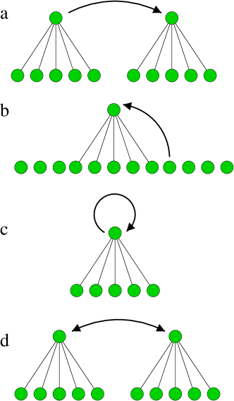
Figure 1: Different kinds of interaction discussed in this contribution: (a) static teacher vs. adaptive student, (b) time series generation and prediction, (c) self-interaction, (d) mutual learning

2 On-line training

The simplest mathematical neural network is the perceptron. It consists of a single layer of $N$ synaptic weights $\underline{w}=(w_{1},...,w_{N})$. For a given input vector $\underline{x}$, the output bit is given by

$$\sigma=\mbox{sign}\left(\sum\limits^{N}_{i=1}\;w_{i}x_{i}\right)$$ (1)

The decision surface of the perceptron is just a hyperplane in the $N$-dimensional input space, $\underline{w}\cdot\underline{x}=0$. A perceptron may also have a continuous output $y$ as

$$y=\tanh\left(\sum\limits^{N}_{i=1}\;w_{i}x_{i}\right)$$ (2)

A perceptron may be considered as an elementary unit of a more complex network like an attractor network or a multilayer network. In fact any function can be approximated by a multilayer network if the number of hidden units is large enough [2].

The perceptron can learn from examples. Examples are input/output pairs,

$$(\underline{x}(t),\underline{\sigma}(t))\;\;\;\qquad t=1,...,\alpha N$$ (3)

On-line training means that at each time step $t$ the weights of the perceptron adapt to a new example, for instance by the rule

$$\underline{w}(t+1)=\underline{w}(t)+\frac{\eta}{N}\sigma(t)\underline{x}(t)\;F(\sigma(t)\underline{x}(t)\cdot\underline{w}(t))$$ (4)

$F(z)=1$ is usually called – after the corresponding biological mechanism – the Hebbian rule, each synapse $w_{i}$ responds to the activities $\sigma(t)x_{i}(t)$ at its ends. $F(z)=\Theta(-z)$ is called the Rosenblatt rule: a training step occurs only if the example is misclassified. Finally, the Adatron rule $F(z)=|z|\Theta(-z)$ is important since it gives good results for generalisation, as discussed in the following. For the last two learning rules, in addition to the two neural activities at the synaptic ends, the postsynaptic potential determines the strength of the synaptic adaptation.

3 Generalisation

Now we consider two perceptrons. One is called the teacher network which is producing a set of examples. It is receiving a set of random input vectors $\underline{x}(t)$ and generating output bits $\sigma(t)$. The teacher has a fixed weight vector $\underline{w}^{T}$.

Each time the teacher is producing a new example, the student perceptron is trained on it according to (4). As a consequence, the weight vector of the student $\underline{w}^{S}(t)$ is time dependent. The student tries to approach the teacher, at each training step $t$ its weight vector moves towards the one of the teacher. It is easy to see that for random inputs $\underline{x}$, equation (4) gives a kind of random walk in $N$-dimensional space with a bias towards the teacher vector $\underline{w}^{T}$.

The distance between student and teacher can be measured by the overlap

$$R=\frac{\underline{w}^{T}\cdot\underline{w}^{S}}{|\underline{w}^{T}||\underline{w}^{S}|}$$ (5)

The quantity $R$ determines the angle $\phi$ between student and teacher weights, $R=\cos\phi$. It turns out that from this overlap the generalisation error $e_{g}$ can be calculated. The generalisation error is the probability that the student gives an answer to a random input $\underline{x}$ which is different from the one of the teacher. One finds

$$e_{g}=\frac{\arccos R}{\pi}$$ (6)

In the limit of infinitely many input units, $N\to\infty$, the dynamics of the overlap $R(t)$ can be calculated analytically. According to (4), the size of the training step scales down with $1/N$. Therefore one defines a variable $\alpha=t/N$ which becomes a continuous variable, called time, in the limit of large $N$.

The time dependence of $R(\alpha)$ is obtained by multiplying (4) by $\underline{w}^{T}$ and $\underline{w}^{S}$ and by averaging these two equations over the random input vector $\underline{x}$. This can be done since the expressions $\underline{w}\cdot\underline{x}$ are Gaussian variables.

For the Adatron rule one finally obtains the differential equation [4]

$$\frac{dR}{d\alpha}=-\frac{R}{2\pi}\arccos{R}+\frac{1}{\pi}\big{(}1-\frac{R^{2}}{2}\big{)}\sqrt{1-R^{2}}$$ (7)

The generalisation error calculated by this equation is shown in Fig. 2. If only a finite number of examples has been learned, $\alpha=0$, the error is 50 %, as bad as random guessing. If the number of training examples is of the order of $N$, $\alpha>0$, the student network has obtained some overlap to the teacher. In the limit of large values of $\alpha$ the error decreases to zero, the student has obtained complete knowledge about the parameters of the teacher.

Figure 2: Generalisation error as a function of time, from Ref. [4]

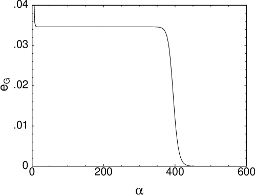
Figure 3: Generalisation error as a function of time, for a multilayer network with two hidden units, from Ref. [7]

The asymptotic decay of the generalisation error depends on the learning rule. One finds for the Adatron rule $e_{g}\propto 3/2\,\alpha^{-1}$. In fact, it has been shown that the error cannot decay faster than $e_{g}\propto 0.88\,\alpha^{-1}$[5]. For the Rosenblatt rule, one finds $e_{g}\propto\alpha^{-1/3}$, and for the Hebbian rule $e_{g}\propto\alpha^{-1/2}$. But in all cases the student succeeds to approach the teacher when it makes of the order of $N$ steps. This even holds when the examples are distorted by noise [6].

Learning from examples works for more complex networks, too. Here I would like to mention the work on specialisation of committee machines [7]. Such a network is a multilayer network with several hidden units, similar to Fig. 8. The output bits of the continuous hidden units are summed and taken as the output of the network. Teacher and student networks have an identical architecture, and the learning step is just a gradient descent of the training error, the quadratic deviation between teacher and student output.

The corresponding generalisation error is shown in Fig. 3. For small number of examples it decreases fast, then it reaches a plateau and only for a huge number of examples it decreases to zero.

The motion of the student network can be expressed by the overlap between the corresponding members of the two machines. The teacher as well as the student consists of two weights vectors, $\underline{w}^{T/S}_{1}$ and $\underline{w}^{T/S}_{2}$. A distance between teacher and student can be defined from the overlaps

$$R_{i,j}=\underline{w}^{T}_{i}\cdot\underline{w}^{S}_{j}$$ (8)

Initially, all vectors are random, hence up to fluctuations all the overlaps are zero. Then all overlaps increase due to learning. But on the plateau of Fig. 3 the overlaps are all identical, $R_{1,1}=R_{2,2}=R_{1,2}$. The student has achieved some knowledge, but it is in a symmetric state. Only if the student receives much more information it can specialise: $R_{1,1}=R_{2,2}$ are much larger than $R_{1,2}$.

In the initial process the two members of the student committee act as being one single perceptron, but later they specialise and follow their partners in the teacher committee until they achieve complete knowledge for $\alpha\to\infty$.

4 Time series prediction and generation

Neural networks are successful prediction algorithms [8]. Given a sequence of numbers, a neural network can be trained on this sequence by moving it over the sequence, as shown in Fig.4. This sequence can be produced by another network, called the teacher, by generating a new number and using it as an input component in the next step. Hence we have a new kind of interacting networks: The teacher with its static weight vector is a bit or sequence generator [9]. The student is adapting its weights to the sequence generated by the teacher.

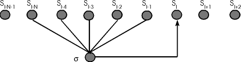
Figure 4: Time series generation and prediction by a perceptron

In principle this is the scenario described in the previous section. Here the difference is that the patterns are correlated, the input is not random but generated from the output of the teacher.

If a neural network cannot generate a given sequence of numbers, it cannot predict it with zero error. Hence one has investigated the generation of time series by neural networks [11, 14, 13, 12] But this is not the whole story. Even if the sequence has been generated by an (unknown) neural network (the teacher), a different network (the student) can try to learn and to predict this sequence. In this context we are interested in two questions:

1. When a student network with the identical architecture as the teacher’s is trained on the sequence, how does the overlap between student and teacher develop with the number of training examples (= windows of the sequence)?

2. After the student network has been trained on a part of the sequence, how well can it predict the sequence several steps ahead?

Recently these questions have been investigated numerically for the simple perceptron, equation (1,2) [10]. Consider a teacher perceptron with weight vector $\underline{w}^{T}$ generating the sequence $S_{0},S_{1},S_{2},...,S_{t},...$ This sequence follows the equation

$$S_{t}=f\left(\frac{1}{N}\sum\limits^{N}_{j=1}\;w_{j}S_{t-j}\right)$$ (9)

where $f(x)$ is the transfer function. It has been shown that a perceptron can generate simple as well as complex sequences [11, 14].

If $f(x)$ is monotonic, for instance $f(x)=\tanh(\beta x)$, then in general one obtains quasiperiodic sequences. In fact, the sequence is essentially generated by one Fourier component of the weight vector $w^{T}_{i}$ [11]. If the transfer function, however, is not monotonic, for instance $f(x)=\sin(\beta x)$, then the sequence can be chaotic, depending on the model parameters [14]. For both cases, learning and prediction have been investigated [10].

If a quasi periodic sequence is learned on-line, using gradient descent to update the weights,

$$\Delta w_{i}=\frac{\eta}{N}(S_{t}-f(h))\cdot f^{\prime}(h)\cdot S_{t-i}\;\;\mbox{with}\;\;h=\beta\sum\limits^{N}_{j=1}w_{j}S_{t-j}$$ (10)

then one has found two time scales (time $\alpha$ means the number of training steps divided by $N$):

1. A short scale on which the overlap $R(\alpha)$ between teacher and student rapidly increases to a value which is still far away from the value $R=1$, which corresponds to perfect agreement.

2. A long one on which the overlap $R(\alpha)$ increases very slowly. Numerical simulations up to $10^{6}N$ training steps yielded an overlap which was close but sell different from the value $R=1$.

Although there is a mathematical theorem on stochastic optimisation which seems to guarantee convergence to perfect success [15], the on–line algorithm cannot gain much information about the teacher network, at least during reasonable training periods.

This is completely different for a chaotic time series generated by a corresponding teacher network with $f(x)=\sin(x)$. It turns out that the chaotic series appears like a random one: After a number of training steps of the order of $N$ the overlap relaxes exponentially fast to perfect agreement between teacher and student.

Hence, after training the perceptron with a number of examples of the order of $N$ we obtain the two cases: For a quasi periodic sequence the student has not obtained much information about the teacher, while for a chaotic sequence the student’s weight vector comes close to the one of the teacher. One important question remains: How well can the student predict the time series?

Figure 5: Prediction error as a function of time steps ahead, for a quasi periodic (lower) and chaotic (upper) series, from Ref.[10]

Fig.5 shows the prediction error as a function of the time interval over which the student makes the predictions. The student network which has been trained on the quasi periodic sequence can predict it very well. The error increases linearly with the size of the interval, even predicting $10N$ steps ahead yields an error of about 10% of the total possible range. On the other side, the student trained on the chaotic sequence cannot make predictions. The prediction error increases exponentially with time; already after a few steps the error corresponds to random guessing, $e_{g}\simeq 1$. The explanation is that an infinitesimal change in the parameters of a chaotic map has the same effect as a small change in initial conditions, namely, an exponential growth in the distance between original and the disturbed trajectory.

In summary one finds the counterintuitive result:

1. A network trained on a quasiperiodic sequence does not obtain much information about the teacher network which generated the sequence. But the network can predict this sequence over many (of the order of $N$) steps ahead.

2. A network trained on a chaotic sequence obtains almost complete knowledge about the teacher network. But this network cannot make reasonable long-term predictions on the sequence.

It would be interesting to find out whether this result also holds for other prediction algorithms, such as multi-layer networks.

5 Self-interaction

In the previous section the time series was generated by a static teacher network. Now we consider a network which changes its synaptic weights while it is generating a bit sequence. The teacher is interacting with itself. The motivation of this investigation stems from the following problem:

Consider some arbitrary prediction algorithm. It may contain all the knowledge of mankind, many experts may have developed it. Now there is a bit sequence $S_{1},S_{2},\dots$ and the algorithm has been trained on the first $t$ bits $S_{1},\dots,S_{t}$. Can it predict the next bit $S_{t+1}$? Is the prediction error, averaged over a large $t$ interval, less than 50%?

If the bit sequence is random then every algorithm will give a prediction error of 50%. But if there are some correlations in the sequence then a clever algorithm should be able to reduce this error. In fact, for the most powerful algorithm one is tempted to say that for any sequence it should perform better than 50% error. However, this is not true [16]. To see this just generate a sequence $S_{1},S_{2},S_{3},\dots$ using the following algorithm:

Define $S_{t+i}$ to be the opposite of the prediction of this algorithm which has been trained on $S_{1},\dots,S_{t}$ .

Now, if the same algorithm is trained on this sequence, it will always predict the following bit with 100% error. Hence there is no general prediction machine; to be successful the algorithm needs some pre-knowledge about the class of problems it is applied to.

The Boolean perceptron is a very simple prediction algorithm for a bit sequence, in particular with the Hebbian on–line training algorithm (4). What does the bit sequence look like for which the perceptron fails completely?

Following (4), we just have to take the negative value

$$S_{t}=-\mbox{sign}\left(\sum\limits^{N}_{j=1}\;w_{j}S_{t-j}\right)$$ (11)

and then train the network on this new bit:

$$\Delta w_{j}=+\frac{1}{N}S_{t}\;S_{t-j}.$$ (12)

The perceptron is trained on the opposite (= negative) of its own prediction. Starting from (say) random initial states $S_{1},\dots,S_{N}$ and weights $\underline{w}$, this procedure generates a sequence of bits $S_{1},S_{2},\dots S_{t},\dots$ and of vectors $\underline{w},\underline{w}(1),\underline{w}(2),\dots\underline{w}(t),\dots$ as well. Given this sequence and the same initial state, the perceptron which is trained on it yields a prediction error of 100%.

It turns out that this simple algorithm produces a rather complex bit sequence which comes close to a random one [17]. After a transient time the weight vector $\underline{w}(t)$ seems to perform a kind of random walk on an $N$–dimensional hyper-sphere. The bit sequence runs to a cycle whose average length $L$ scales exponentially with $N$,

$$L\simeq 2.2^{N}.$$ (13)

The autocorrelation function of the sequence shows complex properties: It is close to zero up to $N$, oscillates between $N$ and $3N$ and it is similar to random noise for larger distances. Its entropy is smaller than the one of a random sequence since the frequency of some patterns is suppressed. Of course, it is not random since the prediction error is 100% instead of 50% for a random bit sequence.

When a second perceptron (=student) with different initial state $\underline{w}^{S}$ is trained on such a anti-predictable sequence generated by Eq.(11) it can perform somewhat better than the teacher: The prediction error goes down to about 78% but it is still larger than 50% for random guessing. Related to this, the student obtains knowledge about the teacher: The angle between the two weight vectors relaxes to about 45 degrees [16, 17]. Hence the complex anti-predictable sequence still contains enough information for the student to follow the time dependent teacher.

6 Agents competing in a closed market

We just considered a network interacting with itself. Now we extend this model to a system of many networks interacting with the minority decision of all members. This work was motivated by the following problem of econophysics [18].

Recently a mathematical model of economy receives a lot of attention in the community of statistical physics. It is a simple model of a closed market: There are $K$ agents who have to make a binary decision $\sigma(t)\in\{+1,-1\}$ at each time step. All of the agents who belong to the minority gain one point, the majority has to pay one point (to a cashier which always wins). The global loss is given by

$$G=\left|\sum\limits^{K}_{t=1}\;\;\sigma(t)\right|$$ (14)

If the agents come to an agreement before they make a new decision, it is easy to minimise $G:(K-1)/2$ agents have to choose $+1$, then $G=1$. However, this is not the rule of the game; the agents are not allowed to make contracts, and communicate only through the global sum of decisions. Each agent knows only the history of the minority decision, $S_{1},S_{2},S_{3},\dots$, but otherwise he/she has no information. Can the agent find an algorithm to maximise his/her profit?

If each agent makes a random decision, then $\langle G^{2}\rangle=K$. It is possible, but not trivial, to find algorithms which perform better than random [19].

Here we use a perceptron for each agent to make a decision based on the past $N$ steps $\underline{S}=(S_{t-N},...,S_{t-1})$ of the minority decision. The decision of agent $\underline{w}(t)$ is given by

$$\sigma(t)=\mbox{sign}(\underline{w}(t)\;\underline{S}).$$ (15)

After the bit $S_{t}$ of the minority has been determined, each perceptron is trained on this new example $(\underline{S},S_{t})$,

$$\Delta\underline{w}(t)=\frac{\eta}{N}\;\;S_{t}\;\underline{S}.$$ (16)

This problem could be solved analytically [20]. The average global loss for $\eta\rightarrow 0$ is given by

$$\langle G^{2}\rangle=(1-2/\pi)K\simeq 0.363\;K.$$ (17)

Hence, for small enough learning rates the system of interacting neural networks performs better than random decisions. Successful cooperation emerges in a pool of adaptive perceptrons.

7 Synchronisation by mutual learning

Before, we have considered a pool of several neural networks interacting through their minority decisions. Now we study the interaction of just two neural networks [20]. Contrary to the teacher/student case, now both of the networks are adaptive, each network is learning the output bit of its partner.

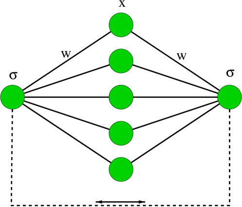
Figure 6: Two perceptrons are trained by their mutual output bits, from Ref. [20]

In particular, we consider the model where two perceptrons $A$ and $B$ receive a common random input vector $\underline{x}$ and change their weights $\underline{w}$ according to their mutual bit $\sigma$, as sketched in Fig. 6. The output bit $\sigma$ of a single perceptron is given by the equation

$$\sigma=\mbox{sign}(\underline{w}\cdot\underline{x})$$ (18)

$\underline{x}$ is an $N$-dimensional input vector with components which are drawn from a Gaussian with mean $0$ and variance $1$. $\underline{w}$ is a $N$-dimensional weight vector with continuous components which are normalised,

$$\underline{w}\cdot\underline{w}=1$$ (19)

The initial state is a random choice of the components $w_{i}^{A/B},i=1,...,N$ for the two weight vectors $\underline{w}^{A}$ and $\underline{w}^{B}$. At each training step a common random input vector is presented to the two networks which generate two output bits $\sigma^{A}$ and $\sigma^{B}$ according to (18). Now the weight vectors are updated by the Rosenblatt learning rule (4):

$$\underline{w}^{A}(t+1) = \underline{w}^{A}(t)+\frac{\eta}{N}\underline{x}\;\sigma^{B}\;\Theta(-\sigma^{A}\sigma^{B})$$

$$\underline{w}^{B}(t+1) = \underline{w}^{B}(t)+\frac{\eta}{N}\underline{x}\;\sigma^{A}\;\Theta(-\sigma^{A}\sigma^{B})$$ (20)

$\Theta(x)$ is the step function. Hence, only if the two perceptrons disagree a training step is performed with a learning rate $\eta$. After each step (7), the two weight vectors have to be normalised.

In the limit $N\rightarrow\infty$, the overlap

$$R(t)=\underline{w}^{A}(t)\;\underline{w}^{B}(t)$$ (21)

has been calculated analytically [20]. The number of training steps $t$ is scaled as $\alpha=t/N$, and $R(\alpha)$ follows the equation

$$\frac{dR}{d\alpha}=(R+1)\left(\sqrt{\frac{2}{\pi}}\;\eta(1-R)-\eta^{2}\frac{\phi}{\pi}\right)$$ (22)

where $\phi$ is the angle between the two weight vectors $\underline{w}^{A}$ and $\underline{w}^{B}$, i.e. $R=\cos\phi$. This equation has fixed points $R=1,R=-1$, and

$$\frac{\eta}{\sqrt{2\pi}}=\frac{1-\cos\phi}{\phi}$$ (23)

Figure 7: Final overlap $R$ between two perceptrons as a function of learning rate $\eta$. Above a critical rate $\eta_{c}$ the time dependent networks are synchronised. From Ref. [20]

Fig.7 shows the attractive fixed point of (22) as a function of the learning rate $\eta$. For small values of $\eta$ the two networks relax to a state of a mutual agreement, $R\rightarrow 1$ for $\eta\rightarrow 0$. With increasing learning rate $\eta$ the angle between the two weight vectors increases up to the value $\phi=133^{\circ}$ for

$$\eta\rightarrow\eta_{c}\cong 1.816$$ (24)

Above the critical rate $\eta_{c}$ the networks relax to a state of complete disagreement, $\phi=180^{\circ},R=-1$. The two weight vectors are antiparallel to each other, $\underline{w}^{A}=-\underline{w}^{B}$.

As a consequence, the analytic solution shows, well supported by numerical simulations for $N=100$, that two neural networks can synchronise to each other by mutual learning. Both of the networks are trained to the examples generated by their partner and finally obtain an antiparallel alignment. Even after synchronisation the networks keep moving, the motion is a kind of random walk on an N-dimensional hypersphere producing a rather complex bit sequence of output bits $\sigma^{A}=-\sigma^{B}$ [17]. In fact, after synchronisation the system is identical to the single network learning its opposite output bit discussed in section 5.

8 Cryptography

In the field of cryptography, one is interested in methods to transmit secret messages between two partners A and B. An opponent E who is able to listen to the communication should not be able to recover the secret message.

Before 1976, all cryptographic methods had to rely on secret keys for encryption which were transmitted between A and B over a secret channel not accessible to any opponent. Such a common secret key can be used, for example, as a seed for a random bit generator by which the bit sequence of the message is added (modulo 2).

In 1976, however, Diffie and Hellmann found that a common secret key could be created over a public channel accessible to any opponent. This method is based on number theory: Given limited computer power, it is not possible to calculate the discrete logarithm of sufficiently large numbers [21].

Recently, it has been shown how interacting neural networks can produce a common secret key by exchanging bits over a public channel and by learning from each other [22].

We want to apply synchronisation of neural networks to cryptography. In the previous section we have seen that the weight vectors of two perceptrons learning from each other can synchronise. The new idea is to use the common weights $\underline{w}^{A}=-\underline{w}^{B}$ as a key for encryption. But two problems have to be solved yet: (i) Can an external observer, recording the exchange of bits, calculate the final $\underline{w}^{A}(t)$, (ii) does this phenomenon exist for discrete weights? Point (i) is essential for cryptography, it will be discussed further below. Point (ii) is important for practical solutions since communication is usually based on bit sequences. It will be investigated in the following.

Synchronisation occurs for normalised weights, unnormalised ones do not synchronise [20]. Therefore, for discrete weights, we introduce a restriction in the space of possible vectors and limit the components $w_{i}^{A/B}$ to $2L+1$ different values,

$$w_{i}^{A/B}\in\{-L,-L+1,...,L-1,L\}$$ (25)

In order to obtain synchronisation to a parallel – instead of an antiparallel – state $\underline{w}^{A}=\underline{w}^{B}$, we modify the learning rule (7) to:

$$\underline{w}^{A}(t+1) = \underline{w}^{A}(t)-\underline{x}\sigma^{A}\Theta(\sigma^{A}\sigma^{B})$$

$$\underline{w}^{B}(t+1) = \underline{w}^{B}(t)-\underline{x}\sigma^{B}\Theta(\sigma^{A}\sigma^{B})$$ (26)

Now the components of the random input vector $\underline{x}$ are binary $x_{i}\in\{+1,-1\}$. If the two networks produce an identical output bit $\sigma^{A}=\sigma^{B}$, then their weights move one step in the direction of $-x_{i}\sigma^{A}$. But the weights should remain in the interval (25), therefore if any component moves out of this interval, it is set back to the boundary $w_{i}=\pm L$.

Each component of the weight vectors performs a kind of random walk with reflecting boundary. Two corresponding components $w_{i}^{A}$ and $w_{i}^{B}$ receive the same random number $\pm 1$. After each hit at the boundary the distance $|w_{i}^{A}-w_{i}^{B}|$ is reduced until it has reached zero. For two perceptrons with a $N$-dimensional weight space we have two ensembles of $N$ random walks on the internal $\{-L,...,L\}$. If we neglect the global signal $\sigma^{A}=\sigma^{B}$ as well as the bias $\sigma^{A}$, we expect that after some characteristic time scale $\tau=\mathcal{O}(L^{2})$ the probability of two random walks being in different states decreases as

$$P(t)\sim P(0)e^{-t/\tau}$$ (27)

Hence the total synchronisation time should be given by $N\cdot P(t)\simeq 1$ which gives

$$t_{\mathrm{sync}}\sim\tau\ln N$$ (28)

In fact, the simulations for $N=100$ show that two perceptrons with $L=3$ synchronise in about 100 time steps and the synchronisation time increases logarithmically with $N$. However, the simulations also showed that an opponent, recording the sequence of $(\sigma^{A},\sigma^{B},\underline{x})_{t}$ is able to synchronise, too. Therefore, a single perceptron does not allow a generation of a secret key.

Obviously, a single perceptron transmits too much information. An opponent, who knows the set of input/output pairs, can derive the weights of the two partners after synchronisation. Therefore, one has to hide so much information, that the opponent cannot calculate the weights, but on the other side one has to transmit enough information that the two partners can synchronise.

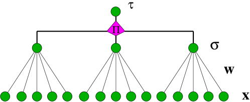
Figure 8: Parity machine with three hidden units.

In fact, it was shown that multilayer networks with hidden units may be candidates for such a task [22]. More precisely, we consider parity machines with three hidden units as shown in Fig.8. Each hidden unit is a perceptron (1) with discrete weights (25). The output bit $\tau$ of the total network is the product of the three bits of the hidden units

$$\tau^{A} = \sigma^{A}_{1}\;\sigma^{A}_{2}\;\sigma^{A}_{3}$$

$$\tau^{B} = \sigma^{B}_{1}\;\sigma^{B}_{2}\;\sigma^{B}_{3}$$ (29)

At each training step the two machines $A$ and $B$ receive identical input vectors $\underline{x}_{1},\underline{x}_{2},\underline{x}_{3}$. The training algorithm is the following: Only if the two output bits are identical, $\tau^{A}=\tau^{B}$, the weights can be changed. In this case, only the hidden unit $\sigma_{i}$ which is identical to $\tau$ changes its weights using the Hebbian rule

$$\underline{w}^{A}_{i}(t+1)=\underline{w}^{A}_{i}(t)-\underline{x}_{i}\tau^{A}$$ (30)

For example, if $\tau^{A}=\tau^{B}=1$ there are four possible configurations of the hidden units in each network:

$(+1,+1,+1),(+1,-1,-1),(-1,+1,-1),(-1,-1,+1)$

In the first case, all three weight vectors $\underline{w}_{i},\underline{w}_{2},\underline{w}_{3}$ are changed, in all other three cases only one weight vector is changed. The partner as well as any opponent does not know which one of the weight vectors is updated.

The partners $A$ and $B$ react to their mutual stop and move signals $\tau^{A}$ and $\tau^{B}$, whereas an opponent can only receive these signals but not influence the partners with its own output bit. This is the essential mechanism which allows synchronisation but prohibits learning. Numerical [22] as well as analytical [23] calculations of the dynamic process show that the partners can synchronise in a short time whereas an opponent needs a much longer time to lock into the partners.

This observation holds for an observer who uses the same algorithm (30) as the two partners $A$ and $B$. Note that the observer knows 1. the algorithm of $A$ and $B$,  2. the input vectors $\underline{x}_{1},\underline{x}_{2},\underline{x}_{3}$ at each time step and   3. the output bits $\tau^{A}$ and $\tau^{B}$ at each time step. Nevertheless, it does not succeed in synchronising with $A$ and $B$ within the communication period.

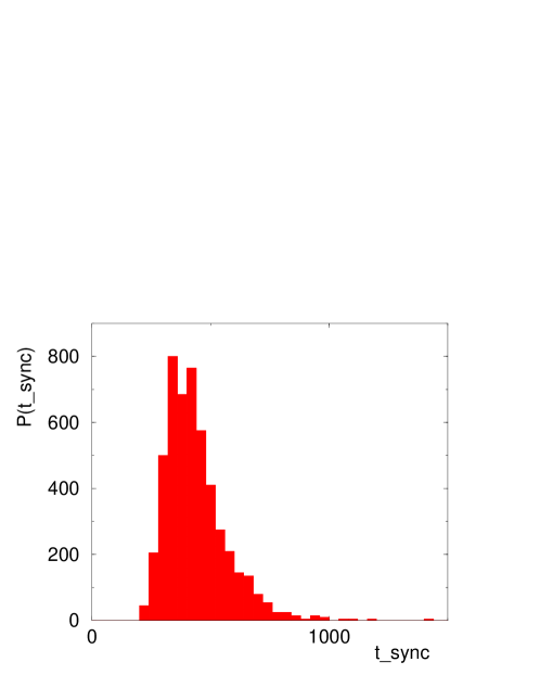
Figure 9: Distribution of synchronisation time for $N=100,L=3$, from Ref.[22]

Figure 10: Average synchronisation time as a function of inverse system size.

Since for each run the two partners draw random initial weights and since the input vectors are random, one obtains a distribution of synchronisation times as shown in Fig. 9 for $N=100$ and $L=3$. The mean value of this distribution is shown as a function of system size $N$ in Fig. 10. Even an infinitely large network needs only a finite number of exchanged bits - about 400 in this case - to synchronise.

If the communication continues after synchronisation, an opponent has a chance to lock into the moving weights of $A$ and $B$. Fig.11 shows the distribution of the ratio between the synchronisation time of $A$ and $B$ and the learning time of the opponent. In the simulations for $N=100$, this ratio never exceeded the value $r=0.1$, and the average learning time is about 50000 time steps, much larger than the synchronisation time. Hence, the two partners can take their weights $\underline{w}^{A}_{i}(t)=\underline{w}^{B}_{i}(t)$ at a time step $t$ where synchronisation most probably occurred as a common secret key. Synchronisation of neural networks can be used as a key exchange protocol over a public channel.

Up to now it is not clear, yet, whether more advanced attacks will finally break this exchange protocol. On the other side, there are several possible extensions of the synchronisation mechanism where tracking seems to be even harder [24].

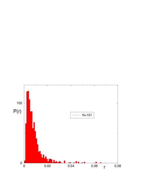
Figure 11: Distribution of the ratio of synchronisation time between networks A and B to the learning time of an attacker E.

9 Conclusions

The dynamics of interacting neural networks has been studied in the context of a simple model: the perceptron and its extensions. The dynamics of these models can be calculated analytically; macroscopic properties can be described by differential equations for a few order parameters.

Several kinds of interaction processes have been studied. In all cases the networks are trained by a set of examples which are generated by different networks. This is the way networks interact. Some networks are generating pairs of high dimensional input data and a corresponding output signal and transmit this information to other networks. The networks receiving this information are adapting their parameters – their synaptic weights – to each example. One question is to what extend the networks exchanging information are approaching each other in the high dimensional synaptic space.

The teacher/student scenario of a static networks generating the examples in addition to an adaptive network being trained on these examples is the case studied most. The question is: How well does the student learn the rule which is producing the examples, how can it generalise? The analytic solutions for the perceptron show the number of training examples has to be of the number of neurons to achieve generalisation. For the optimal training algorithm the generalisation error decays not faster than the inverse power of training time.

If both teacher and student networks are more complex then new phenomena are observed. For example, for a committee machine specialisation occurs: For short times the student relaxes fast to a configuration for which it has achieved generalisation but it is still in a symmetric state, it behaves like a simple perceptron. Only if the number of examples is increased to a very large value the student network can escape from this configuration and each member of the committee specialises to its corresponding member in the teacher network.

A static teacher network can also generate a time series on which the student network is trained. In addition to the overlap between teacher and student parameters, one is interested in the prediction abilities of the student after the interaction period. It turns out that learning and prediction are not necessarily correlated. One finds perceptrons which learn a chaotic sequence very well but cannot predict it. On the other side, for quasiperiodic sequences it is difficult to learn the weights of the teacher but it is simple to predict the corresponding sequence.

A very general question about properties of prediction algorithms leads to a perceptron interacting with itself. It produces a rather complex time series which yields 100 % prediction error if the same perceptron is trained on this sequence. But even if a different perceptron is trained on this sequence, it achieves some knowledge about the teacher, hence its prediction error is larger than 50 %.

A community of neural networks can exchange information and learn from each other. It is shown how such a scenario can lead to successful cooperation in the minority game – a model for competing agents in a closed market.

If two networks are exchanging information and learning from each other, they can synchronise. That means, after some training time they relax to a configuration with identical time dependent synaptic weights (up to a common sign). The two networks keep diffusing on a high dimensional hypersphere, but with identical weights. Neural networks can synchronise by mutual learning.

This new phenomenon is applied to cryptography. It is shown how multilayer networks with discrete weights synchronise after a few hundred steps of interactions. However, a third network which is recording the exchange of examples does not synchronise, at least during a short period of time. Learning by mutual learning is fast, but learning by listening is very slow. Hence two partners can agree on a common secret key over a public channel. Any observer who knows all the details of the algorithm and who knows all the training examples cannot calculate the secret key. This is – to my knowledge – the first public key exchange which is not based on number theory. Future research will show how well this new algorithm – based on mutual learning of neural networks – can resist any advanced attacks which still have to be invented.

Synchronisation of neural networks is an active subject of research in neurobiology. Up to now it is – to my knowledge – unclear how synchronisation develops and what is its function. Here the model calculations point to a new direction: Two or several biological networks can achieve a common time dependent state by learning information exchanged between active partners. Any other network receiving the same information without being able to influence the partners cannot lock into this time dependent common state. Hence even in a fully connected network, parts of it can synchronise by mutual learning, at the same time screening their synchronised state from parts which learn only by listening.

In summary, this is the first attempt to develop a theory of interacting neural networks. Several phenomena were discovered from simple models like the perceptron or the parity machines. These phenomena were neither included into the models from the beginning nor are obvious; they are a result of cooperative behaviour of the synaptic weights and can only be understood from the analytical and numerical calculations.

As the different scenarios described in this overview show, the first results of this theory of interacting adaptive systems may be relevant in the fields of cooperative systems, nonlinear dynamics, time series prediction, economic models, biological networks and cryptography.

Acknowledgement This overview is based on enjoyable collaborations with Ido Kanter, Richard Metzler and Michal Rosen-Zvi. I thank Michael Biehl for suggestions on the manuscript. This work has been supported by the German Israel Science Foundation (GIF), the Minerva Center of the Bar Ilan University and the Max-Planck Institute für Physik komplexer Systeme in Dresden.

References

- [1] Hertz, J., Krogh, A., and Palmer, R.G.: Introduction to the Theory of Neural Computation, (Addison Wesley, Redwood City, 1991)
- [2] Engel, A., and Van den Broeck, C.: Statistical Mechanics of Learning, Cambridge University Press, 2001)
- [3] Biehl, M., and Caticha, N.: Statistical Mechanics of On-line Learning and Generalisation, The Handbook of Brain Theory and Neural Networks, ed. by M. A. Arbib (MIT Press, Berlin 2001)
- [4] Biehl,M. and Riegler,P.: On-line learning with a perceptron Europhys. Lett. 28, 525 (1994)
- [5] Kinouchi, O. and Caticha, N. Optimal generalisation in perceptrons, J. Phys. A 25, 6243 (1992)
- [6] Biehl,M., Riegler,P. and Stechert,M.: Learning from noisy data: An exactly solvable model, Phys. Rev. E 52, 4624 (1995)
- [7] Biehl,M. Riegler,P. and Wöhler,C.: Transient dynamics of on-line learning in two-layered networks J. Phys A 29,4769 (1996); Saad, D. and Solaa, S.A., On-line learning in soft committee machines, Phys. Rev. E 52, 4225 (1995)
- [8] Weigand, A. and Gershenfeld, N.S.: Time Series Prediction, Addison Wesley, Santa Fe (1994)
- [9] Eisenstein, E., Kanter, I., Kessler, D.A., and Kinzel, W.: Generation and Prediction of Time Series by a Neural Network, Phys. Rev. Letters 74 1, 6-9 (1995)
- [10] Freking, A., Kinzel, W., and Kanter, I.: cond-mat/
- [11] Kanter, I., Kessler, D.A., Priel, A., and Eisenstein, E.: Analytical Study of Time Series Generation by Feed-Forward Networks, Phys. Rev. Lett. 75 13, 2614-2617 (1995)
- [12] Schröder, M. and Kinzel, W.: Limit cycles of a perceptron, J. Phys. A 31, 9131-9147 (1998)
- [13] Ein-Dor, L., and Kanter, I.: Time Series Generation by Multi-layer networks, Phys. Rev. E 57, 6564 (1998)
- [14] Priel, A., and Kanter, I.: Robust chaos generation by a perceptron, Europhys. Lett. 51, 244-250 (2000)
- [15] C. M. Bishop: Neural Networks for Pattern Recognition (Oxford University Press, New York 1995)
- [16] Zhu, H., and Kinzel, W.: Anti-Predictable Sequences: Harder to Predict Than A Random Sequence, Neural Computation 10, 2219-2230 (1998)
- [17] Metzler, R., Kinzel, W., Ein-Dor, L., and Kanter, I.: Generation of unpredictable time series by a neural network, Phys. Rev. E 63, 056126 (2001).
- [18] Econophysics homepage: http://www.unifr.ch/econophysics/
- [19] Challet, D., Marsili, M., and Zecchina, R.: Statistical Mechanics of Systems with Heterogeneous Agents: Minority Games, Phys. Rev. Lett. 84 8, 1824-1827 (2000)
- [20] Metzler, R., Kinzel, W., and Kanter, I.: Interacting Neural Networks, Phys. Rev. E 62, 2555 (2000)
- [21] D. R. Stinson, Cryptography: Theory and Practice (CRC Press 1995)
- [22] I. Kanter, W. Kinzel and E. Kanter, Secure exchange of information by synchronisation of neural networks Europhys. Lett. 57, 141-147 (2002)
- [23] M. Rosen-Zvi, I. Kanter and W. Kinzel, cond-mat/0202350 (2002)
- [24] Kanter,I. and Kinzel, W.: unpublished