Quantum Monte Carlo study of the three-dimensional attractive Hubbard model

Abstract

We study the three-dimensional (3D) attractive Hubbard model by means of the Determinant Quantum Monte Carlo method. This model is a prototype for the description of the smooth crossover between BCS superconductivity and Bose-Einstein condensation. By detailed finite-size scaling we extract the finite-temperature phase diagram of the model. In particular, we interpret the observed behavior according to a scenario of two fundamental temperature scales; $T^{*}$ associated with Cooper pair formation and $T_{c}$ with condensation (giving rise to long-range superconducting order). Our results also indicate the presence of a recently conjectured phase transition hidden by the superconducting state. A comparison with the 2D case is briefly discussed, given its relevance for the physics of high-$T_{c}$ cuprate superconductors.

The existence of a smooth crossover between the two paradigms of quantum superfluidity, the Bardeen-Cooper-Schrieffer (BCS) superconductivity and the Bose-Einstein condensation (BEC) is firmly established legett ; nsr . In this context, the attractive Hubbard model (AHM) has appeared as an ideal presentation of the whole evolution between the BCS and BEC physics randeria . A concrete property of this Hamiltonian is the existence of two (not always) distinct energy scales: one associated with the formation of Cooper pairs ($T^{*}$) and another with the onset of long-range order in the system ($T_{c}$) ranninger . Although their qualitative behavior is well-known, a quantitative determination is still missing, due to the fact that it is hard to access the intermediate regime by a controlled approximation scheme. In this respect the Determinant Quantum Monte Carlo (DQMC) method hirsch ; lohgub is a powerful tool as it provides results free of systematic errors. A detailed finite-size analysis is however necessary in order to extract the thermodynamic limit properties, which can then be compared with the outputs of other methods recently applied to the same problem keller ; capone . At this point we should stress the role of dimensionality that determines the nature of the superconducting phase transition at $T_{c}$; the strictly 2D realization of the model is characterized by a Berezinskii-Kosterlitz-Thouless type phase transition, whereas the 3D case displays a “normal” second-order one, which is more easily accessible by DQMC. Since the intermediate regime of the AHM constitutes the simplest model for a short-coherence-length superconductor, the considerations presented hereafter may as well help to clarify the influence of the dimensionality on some properties exhibited by the 3D strongly anisotropic high-$T_{c}$ superconductors.
In this Letter, we present the results of extensive DQMC simulations for the finite-temperature properties of the AHM in three dimensions. In spite of finite-size effects, we show that it is possible by a scaling analysis to quantitatively establish the phase diagram of $T_{c}(U,n)$ as a function of the interaction strength and density of a model that exhibits a genuine second-order phase transition (unlike its 2D version). Furthermore, the pair formation temperature $T^{*}$ is studied in detail, revealing the existence of a transition in the non-superconducting state taking place at a critical coupling strength. These results complete recent calculations which have postulated the existence of such a transition in the infinite-dimension version of the model keller ; capone .
Model and method. — The attractive Hubbard model is defined by the following Hamiltonian,

$$\mathcal{H}=-t\sum_{<i,j>,\sigma}(c_{i\sigma}^{\dagger}c_{j\sigma}+\mbox{H.c.})-U\sum_{i}n_{i\uparrow}n_{i\downarrow}-\mu\sum_{i,\sigma}n_{i,\sigma},$$ (1)

where $<i,j>$ denotes a pair of nearest neighbors on a cubic lattice with $N=L^{3}$ sites, $c_{i\sigma}^{\dagger}(c_{i\sigma})$ is a fermion creation (annihilation) operator of spin $\sigma=\uparrow\downarrow$ and $n_{i,\sigma}=c_{i\sigma}^{\dagger}c_{i\sigma}$. We take $t>0$, $U>0$ and the chemical potential $\mu$ is tuned to yield a fixed density $0<n<2$. Outside half-filling ($n\neq 1$) this model presents a finite-temperature transition into a phase characterized by long-range $s$-wave superconducting order associated with the breaking of the U(1) gauge symmetry.
To study the finite temperature properties of this system we use the conventional DQMC hirsch ; lohgub simulation method. Since the attractive interaction does not lead to a minus-sign problem, the whole $U$-$n$-$T$ phase diagram can be reliably studied. Because of the grand-canonical nature of DQMC, it is necessary to estimate the function $\mu=\mu(T,n,U,L)$ in order to work at a fixed density $n$. This presents a considerable load in this work compared to similar DQMC simulations at half-filling staudt . Typically we take $n=0.5$ (quarter-filling) for which results using other methods have already been presented keller ; capone . We also restrict ourselves to finite-temperature static correlation functions lohgub , such as the $s$-wave pair-pair correlation function $C_{\Delta}$ and the Pauli spin susceptibility $\chi_{P}$, given by:

$$C_{\Delta}(T,N) = \frac{1}{N}\sum_{i,j}\langle\Delta_{i}\Delta_{j}^{\dagger}+\Delta_{j}\Delta_{i}^{\dagger}\rangle$$ (2)

$$\chi_{P}(T,N) = \frac{1}{T}\,\frac{1}{N}\sum_{i,j}\langle\mathbf{S}_{i}\cdot\mathbf{S}_{j}\rangle.$$ (3)

Here $\Delta_{i}=c_{i\uparrow}c_{i\downarrow}$ and $\mathbf{S}_{i}=\sum_{\mu,\nu=\uparrow,\downarrow}c_{i\mu}^{\dagger}\boldsymbol{\sigma}_{\!\mu\nu}c_{i\nu}$, $\boldsymbol{\sigma}$ being the vector of Pauli matrices. $C_{\Delta}$ allows to determine the superconductiong transition temperature $T_{c}$, since it signals the breaking of the U(1) gauge symmetry. We recall that this approach is not applicable to the strictly 2D case where more sophisticated quantities have to be calculated fakher . On the other hand $\chi_{P}$ indicates the presence of pairing in the system, related to the temperature scale $T^{*}$ as discussed below.
Regarding the DQMC simulations, the imaginary time discretization is $\Delta\tau=0.125t^{-1}$ and lattices of size $N=4^{3}-10^{3}$ (with periodic boundary conditions) are considered in order to keep the CPU time into reasonable limits. Two types of finite-size effects are present: first, the discreteness of the spectrum introduces artificial features at low temperatures $T\lesssim 0.1t$ and weak couplings $U\lesssim 2t$ (signaled by $(\frac{\partial\mu}{\partial T})_{n}>0$); second, the superconducting phase transition is rounded and corresponds to the point where the correlation length $\xi(T)$ becomes larger than the linear system size $L$.
Determination of $T_{c}$. — Extracted by finite-size analysis of very good quality data, the value of $T_{c}$ is in principle free of systematic errors, except a small uncertainty ($\lesssim 5$ percents) due to the statistical error and to the finite imaginary time discretization $\Delta\tau>0$. Given $U$ and $n$, the pair-pair correlation function $C_{\Delta}$ (Eq.2) is evaluated for various temperatures $T$ and sizes $N$. This shows clearly that $C_{\Delta}$ is characterized by a low- and a high-temperature regime, related by a transition region that becomes sharper and sharper as $N$ increases. The latter observation agrees well with the behavior expected in the thermodynamic limit, where $C_{\Delta}$ displays a discontinuous derivative at the phase transition and becomes non-zero only below $T_{c}$. This behavior, typical for all the parameter values used in our calculations, is shown in Fig. 1 for the special case $U=6t$ and $n=0.5$.

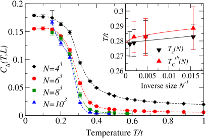
Figure 1: Main: temperature and size dependences of the pair-pair correlation function (2) for the case $U=6t$ and $n=0.5$. Inset: extrapolation to the thermodynamic limit of the size-dependent critical temperatures $T_{c}(N)$ and $T_{c}^{th}(N)$, same $U$ and $n$.

Although it does not correspond to a genuine phase transition, it allows to define a size-dependent transition temperature $T_{c}(N)$ which we can use to deduce the value of $T_{c}\equiv T_{c}(\infty)$. A convenient choice for $T_{c}(N)$ is given by the inflexion point of the curve $C_{\Delta}(T,N)$ versus $T$ obtained by a (stable) Lagrange polynomial interpolation of the DQMC data. Plotting the obtained $T_{c}(N)$ versus $N^{-1}$, we extrapolate to $N\rightarrow\infty$ using a linear fit of the data, as shown in the inset of Fig. 1. The validity of this procedure is confirmed by the evaluation of the specific heat $c_{V}(T)$ whose well-defined peak can be used to define another size-dependent critical temperature $T_{c}^{th}(N)$. $c_{V}(T)$ is obtained by the numerical derivative of the expectation value of the energy thesis . A fit of the values for $T_{c}^{th}(N)$ with a functional form $T_{c}(\infty)=T_{c}^{th}(N)+\mathcal{O}(\frac{1}{\sqrt{N}})$ (corresponding to a superconducting phase transition in the universality class of the 3D $XY$ model engelbrecht ; schneider ) is shown on the inset of Fig. 1. It reveals that the finite-size corrections to $T_{c}$ are very weak and in particular not larger than the statistical errors resulting from the DQMC method. Thus both approaches presented above are fully compatible and yield an uncertainty on the extrapolated value of $T_{c}$ which is typically of the order of 5 percent.
The critical temperature $T_{c}(U,n)$. — The above procedure, applied to a range of parameters $U$ and $n$, determines quantitatively the $U$-$n$-$T_{c}$ phase diagram of the AHM. First we consider half-filling (i.e. $n=1$) which provides a useful check for our method. This case is equivalent to the repulsive model that has been recently studied by Staudt et al. using the same method staudt . The agreement on the values of $T_{c}(U,n=1)$ is almost perfect thesis ; a small difference ($<3$ percents) appearing systematically is due to the extrapolation $\Delta\tau\rightarrow 0$ performed by these authors and not done here due to calculation time restrictions. Turning now to quarter-filling, we obtain the results presented on Fig. 2. Before discussing the intermediate $U$ regime, we observe that,

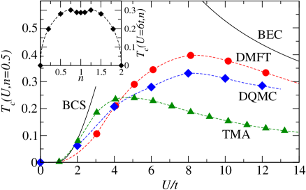
Figure 2: DQMC results for the critical temperature $T_{c}(U,n)$ and comparison with other methods keller . Main: dependence on the coupling $U$. Inset: dependence on the density $n$.

as long as the DMQC method works properly ($2t\leq U\leq 12t$), the extreme values of $T_{c}(U)$ are joining progressively the corresponding asymptotic curves, given by the BCS gap equation for small $U$ and by the 3D BEC formula for large $U$. Their respective dependences in $U$ follow essentially $T_{c}\propto\exp(1/U)$ and $T_{c}\propto 1/U$, with the assumption that in the latter case the bosons are noninteracting and have an effective hopping amplitude $t_{B}=2t^{2}/U$. In the crossover region we observe, as expected, a smooth interpolation between the BCS and BEC regimes, with a maximal value of $T_{c}=0.35t$ situated at $U\simeq 8t$. It is now interesting to compare our results with those proposed in recent works. In Fig. 2 the data obtained using the Dynamical Mean-Field Theory (DMFT) and a $\mathbf{k}$-independent $T$-matrix approximation (TMA) keller are also plotted, rescaled by a factor $\sim 2$ so that the dimensionless product $U$ times the density of states at the Fermi level is the same as in our model thesis ; dos . Similarly to the half-filling case staudt , we observe a good overall agreement with DMFT results, the discrepancy at strong coupling ($U>6t$) being attributed to the mean-field character of DMFT; on the other hand TMA clearly fails outside the BCS regime. We also mention a recent $\mathbf{k}$-dependent $T$-matrix calculation engelbrecht for $U=4t$ with a $T_{c}$ in quantitative agreement with our results.
In addition to $U$, $T_{c}$ also depends upon the density $n$. Our results show that the function $T_{c}(U=\mbox{const.},n)$ is not monotonic dossantos in $0\leq n\leq 1$ ($1\leq n\leq 2$) unlike it was previously assumed ranninger . The maximal transition temperature for a given $U$ is situated around $n=0.75$ ($1.25$). This feature is illustrated on Fig. 2 for the case $U=6t$ and is reminiscent of the two-dimensional case where the higher symmetry of the Hamiltonian (1) at half-filling (SO(3) instead of U(1)) reduces $T_{c}$ to zero, as discussed recently tremblay . The appearance of an additional charge-density wave (CDW) ordering has been studied by means of the corresponding static correlation function thesis .
The pairing temperature scale $T^{*}(U,n)$.— As mentioned previously, $T^{*}$ is besides $T_{c}$ another temperature scale that characterizes the BCS-BEC crossover. In the case of the AHM, $T^{*}$ can be interpreted within a pairing scenario as signaling a re-arrangement of fermionic quasiparticles into $s$-wave singlet pairs. As a consequence, the spectral weight of low-energy spin excitations is reduced and the spin response weakens. This process can be studied by considering the Pauli susceptibility $\chi_{P}$ (Eq. 3). Although $T^{*}$ may not always correspond to a single point, but to an extended energy scale, it can nevertheless be identified with the position of the maximum of $\chi_{P}(T)$ dossantos . This definition has the advantage of satisfying the expected asymptotic behavior of $T^{*}$, i.e. $T^{*}=T_{c}$ in the BCS case and $T^{*}\propto U/\ln(U/\epsilon_{F})^{3/2}$ for the BEC limit randeria . The way the Pauli spin susceptibility evolves between these two regimes is shown on Fig. 3.

Figure 3: Pauli susceptibility $\chi_{P}$. Top: $T$ dependence for various values of $U$ (size $N=6^{3}$). Bottom: $T$ and $N$ dependence close to the transition temperature and separation of $T_{c}$ and $T^{*}$, same symbols as in Fig. 1 ($n=0.5$ for both cases).

It is instructive to analyze these DQMC results by considering the sensitivity of $T^{*}$ to finite-size effects. For the “weak coupling” case $U\leq 4t$, one observes that the shape of $\chi_{P}(T)$ in the region around its maximal value depends strongly on the system size $N$, becoming sharper as $N$ increases. In this case the extracted value of $T^{*}$ turns out to be nearly equal to $T_{c}$, given the accuracy on the numerical results ($\lesssim 5$ percents). On the other hand, a “strong coupling” behavior appears for $U\geq 5t$, characterized by a much smoother susceptibility around its maximum. In this region finite-size effects have disappeared, indicative of an effect characterized by a short coherence length. Here, $T^{*}$ is definitely different from $T_{c}$. In the interval $[T_{c},T^{*}]$ the interesting phenomenon of precursor pairing takes place, a point which will be further discussed below. We can thus present the complete phase diagram on Fig.4 by adding the function $T^{*}(U,n=\text{const.})$

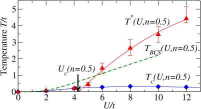
Figure 4: $U$-$T$ phase diagram of the 3D attractive Hubbard model at quarter-filling. The errorbars correspond to the temperature interval around $T^{*}$ where $\chi_{P}(T)$ is less than one percent smaller than its maximal value, giving thereby an idea of the temperature range associated with $T^{*}$.

that clearly displays the two different regimes described above. In the weak coupling regime one observes that $T^{*}$ does not correspond to a BCS critical temperature extrapolated at $U\geq 2t$. On the strong coupling side $T^{*}$ defines an energy scale, which is approximately quantified by the errobars on Fig.4, and resembles to a straight line situated below the diagonal, in qualitative agreement with the asymptotic expression given above.
Discussion.— A first remark concerns the recent observation of a (first-order) phase transition in the non-superconducting solution of the AHM keller ; capone . Since this state is metastable below $T_{c}$, it cannot be accessed by DQMC (applying a magnetic field would cause a minus-sign problem). However the manifestations of this transition may be present above $T_{c}$ as well and the previous analysis of the Pauli spin susceptibility constitutes an ideal illustration. Indeed, it turns out that the high-temperature behavior of $\chi_{P}(T)$, observed for $U\leq 4t$ and characterized by a monotonic decrease with $T$, may correspond to a Fermi liquid normal state where the interaction amounts only to a renormalization of parameters. On the other hand, the regime $U\geq 5t$, which displays the phenomenon of precursor pairing for $T_{c}<T\lesssim T^{*}$, fits well to a phase containing “incoherent pairs” keller ; capone . Consequently a “critical” coupling strength $U_{c}$ may be situated around $U=(4.3\pm 0.1)t$, as it can be deduced by extrapolation at $T=0$ on Fig. 4. This value argrees very well with the (rescaled) DMFT result $0.56\times W\times 2\approx 4.5t$, $W=4t$ being the bandwidth keller ; dos . One also remarks that $U_{c}$ does not correspond to the point where the chemical potential $\mu$ (including the Hartree shift $-U/2$) becomes lower than the bottom of the non-interacting band (for $n=0.5$, we would get $U_{c}\approx 10t$). In fact, to our knowledge, there exists no criterion that yields a good estimate of $U_{c}$ in three dimensions.
In contrast to 3D where the effects of the thermal pairing fluctuations are rather weak babaev ; preosti , in 2D they are very important schneider leading apparently to a $T^{*}$ joining smoothly $T_{c}$ singer . This confirms the observation by Moukouri et al. moukouri that precursor phenomena in the AHM have two origins: enhanced thermal pairing fluctuations (in 2D only) and a strong pairing interaction (in both cases). The fact that the AHM contains a transition between a Fermi liquid and a state of “incoherent pairs” may be of interest in the context of the high-$T_{c}$ superconductors phase diagram, where the scenario of a hidden quantum phase transition has been proposed loram . Of course the driving parameter in this case is the doping and the symmetry of the superconducting phase is $d$-wave.

- (1) A. J. Legett, in Modern Trends in the Theory of Condensed Matter, edited by A. Pekalski and R. Przystawa (Springer Verlag, 1985).
- (2) P. Nozière and S. Schmitt-Rink, J. Low Temp. Phys. 59, 195 (1985).
- (3) M. Randeria, in Bose-Einstein Condensation, edited by A. Griffin, D. Snoke, and S. Stringari (Cambridge University Press, 1994).
- (4) R. Micnas, J. Ranninger, and S. Robaszkiewicz, Rev. Mod. Phys. 62, 113 (1990).
- (5) J. E. Hirsch, Phys. Rev. B 28, 4059 (1983).
- (6) E. Y. Loh and J. E. Gubernatis, in Electronic Phase Transitions, edited by W. Hanke and Y. V. Kopaev (Elsevier Science Publishers, 1992).
- (7) M. Keller, W. Metzner, and U. Schollwock, Phys. Rev. Lett. 86, 4612 (2001).
- (8) M. Capone, C. Castellani, and M. Grilli, Phys. Rev. Lett. 88, 126403 (2002).
- (9) R. Staudt, M. Dzierzawa, and A. Muramatsu, Eur. Phys. J. B 17, 411 (2000).
- (10) F. F. Assaad, W. Hanke, and D. J. Scalapino, Phys. Rev. B 50, 12835 (1994).
- (11) A. Sewer, Ph.D. thesis, Université de Neuchâtel (2001).
- (12) J. R. Engelbrecht and H. Zhao, eprint cond-mat/0110356.
- (13) T. Schneider and J. M. Singer, Phase transtion approach to high temperature superconcuctivity (Imperial College Press, 2000).
- (14) It would be interesting to compare the DQMC data with DMFT results obtained using a more realistic density of states, e.g. corresonding to a 3D tight-binding system, rather than the elliptic one used in keller . .
- (15) R. dos Santos, Phys. Rev. B 50, 635 (1994).
- (16) S. Allen, H. Touchette, S. Moukouri, Y. M. Vilk, and A. M. S. Tremblay, Phys. Rev. Lett. 83, 4128 (1999).
- (17) E. Babaev, Phys. Rev. B 63, 184514 (2001).
- (18) G. Preosti, Y. M. Vilk, and M. R. Norman, Phys. Rev. B 59, 1474 (1999).
- (19) J. M. Singer, T. Schneider, and M. H. Pedersen, Eur. Phys. J. B 2, 17 (1998).
- (20) S. Moukouri, S. Allen, F. Lemay, B. Kyung, D. Poulin, Y. M. Vilk, and A. M. S. Tremblay, Phys. Rev. B 61, 7887 (2000).
- (21) J. L. Tallon and J. W. Loram, Physica C 318, 194 (2001).