On Rényi entropies characterizing the shape and the extension of the phase space representation of quantum wave functions in disordered systems

Abstract

We discuss some properties of the generalized entropies, called Rényi entropies and their application to the case of continuous distributions. In particular it is shown that these measures of complexity can be divergent, however, their differences are free from these divergences thus enabling them to be good candidates for the description of the extension and the shape of continuous distributions. We apply this formalism to the projection of wave functions onto the coherent state basis, i.e. to the Husimi representation. We also show how the localization properties of the Husimi distribution on average can be reconstructed from its marginal distributions that are calculated in position and momentum space in the case when the phase space has no structure, i.e. no classical limit can be defined. Numerical simulations on a one dimensional disordered system corroborate our expectations.

I Introduction

The measure of the extension of phase space distribution of quantum states tells us important information on the degree of ergodicity and at the same time the degree of localization. These information are directly connected to the caoticity of the underlying classical dynamics if the latter is meaningful. In the ergodic regime trajectories visit every corner of phase space hence the quantum states associated to such orbits are expected to be extended. On the other hand regular islands trap classical trajectories and the corresponding states are localized. Therefore the extension properties of the eigenstates directly reflect the nature of classical dynamics. For this purpose the Shannon entropy or information content has been used widely as a measure of complexity of quantum states. This and other generalized entropic measures have been invoked by Życzkowsky in Ref. karol90, as measures of chaotic signatures. In subsequent work karolphe this idea has been elaborated further and a direct correspondence between the complexity of quantum states and the underlying dynamics has been demonstrated in particular by projecting the quantum states onto a coherent state basis. Recently other works have showed the renewed interest in this field AH ; Korsch ; Karol01 ; sugita . We have to emphasize, however, that even systems without classical limit, e.g. disordered systems, have been involved in such phase space studies dietmar ; wobst ; heis . This latter topic is the main motivation of our present work as well.

In the present work we give further arguments in favor of the application of generalized entropies, the Rényi entropies, for the characterization of quantum phase space distributions, however, we point out some problems in connection to the calculation of these parameters for continuous distributions. As a remedy for these problems we show that the differences of Rényi entropies are on the other hand free from these anomalies.

Furthermore we will show that indeed these entropic measures give important information concerning the localization properties of phase space distributions especially the Husimi distribution. We will also give arguments and numerical proofs that in fact in the case of wave functions of disordered systems there is no need to calculate the Husimi distributions themselves especially because the average localization properties of the Husimi functions of a set of states can be obtained from the average properties of the marginal distributions of the Husimi functions.

Using different techniques similar results have been obtained for a particular quantity, the participation ratio in Refs. sugita, ; wobst, . Our approach, however, is more general.

In the next section we introduce the basic ideas and tools that have been widely used in the literature, namely the participation number (ratio) and the Shannon entropy for the case of discrete distributions. We also show that these quantities give roughly the same information, however, using these parameters a new quantity, the structural entropy, can be defined that contains important information concerning the shape of a distribution. It is also shown that these parameters are nothing else but some special cases of the differences of Rényi entropies. Section II contains merely the revision of what has been published before and we conclude this section analyzing the problem of continuous distributions and showing that the above mentioned differences of Rényi entropies are free from the divergences. In Section III we elaborate the appropriate generalization of these parameters for continuous distributions. In Section IV we introduce the Husimi representation of quantum states and describe some of its properties. In Section V Rényi entropies are applied for Husimi distributions and it is shown that the properties of its marginal distributions already give a qualitative picture that for special cases may quantitatively be correct, as well. In Sect. VI numerical simulations for the one dimensional Anderson model provide important verification of the results presented in Sect. V. Finally some concluding remark are left for Sect. VII.

II Basic ideas

The extension of a discrete distribution of a state is often characterized by its entropy, $S$, or by its second moment, $D$. Both of these quantities, i.e. $\exp(S)$ and $D$ practically measure the same thing, namely the number of amplitudes that mainly contribute to the expansion of the state over a suitable basis.

Let us consider a wave function $\Psi$ that is represented by its expansion over a complete basis set on a finite grid of $N$ states $\phi_{i}$

$$\Psi=\sum_{i=1}^{N}c_{i}\phi_{i}\qquad\mbox{with}\qquad\sum_{i=1}^{N}|c_{i}|^{2}=1$$ (1)

Note that each of the coefficients, $Q_{i}=|c_{i}|^{2}$, obey the condition

$$0\leq Q_{i}\leq 1,$$ (2)

and they sum up to unity. Then the usual definitions of participation number, $D$, and entropy, $S$ are

$$D^{-1}=\sum_{i=1}^{N}Q_{i}^{2}\qquad\mbox{and}\qquad S=-\sum_{i=1}^{N}Q_{i}\ln Q_{i}.$$ (3)

The parameter $D$ tells us how many of the numbers $Q_{i}$ are significantly larger than zero. For example if only one of them is unity and the rest is zero, then $D=1$. Otherwise if $Q_{i}=1/N$ homogeneously, then we get $D=N$. Similar properties can be shown to hold for $\exp S$, therefore it is easy to show that the two quantities provide roughly the same information

$$S\approx\ln D,$$ (4)

i.e. both, $S$ and $\ln D$ describe the extension of the discrete distribution. That is the reason for calling $D$ as the number of principal components. The close relation between $S$ and $D$, Eq. (4), has often been overlooked and presented manyb ; Felix as an interesting similarity. However, as it has been demonstrated in Ref. PV92, and applied in several studies later PV92 ; other2 ; quchem ; dqp ; spst , the difference

$$S_{str}=S-\ln D$$ (5)

is a meaningful and most importantly a nonnegative quantity that turns out to be very useful in the characterization of the shape of the distribution of the probabilities $Q_{i}$. That is the reason why it has been termed as structural entropy of a distribution. Moreover the value of the participation number normalized to the number of available components is an important partner quantity

$$q=\frac{D}{N},$$ (6)

which has been termed as the participation ratio in the literature. These two quantities satisfy the following inequalities PV92

$$0< q \leq 1$$ (7a)

$$0\leq S_{str} \leq-\ln q.$$ (7b)

Generalized entropies have been introduced by Rényi renyi in the form of

$$R_{m}=\frac{1}{1-m}\ln\sum_{i=1}^{N}Q_{i}^{m},$$ (8)

that monotonously decreases for increasing $m$. For the special cases of $m=0$, $1$, and $2$ we recover the total number of components, the Shannon-entropy and the participation number

$$R_{0}=\ln N\qquad\lim_{m\to 1}R_{m}=S,\qquad R_{2}=\ln D.$$ (9)

Notice that the order $m$ in (8) is not necessarily integer. We can readily realize that the parameters, (5) and (6), are nothing else but the differences other2 of the special cases of $R_{0}$, $R_{1}$, and $R_{2}$, i.e.

$$S_{str} = R_{1}-R_{2}$$ (10a)

$$-\ln q = R_{0}-R_{2}.$$ (10b)

A number of applications have been presented to date other2 showing their diverse applicability starting from quantum chemistry quchem up to localization in disordered and quasiperiodic systems dqp up to the statistical analysis of spectra spst .

In the present work we are going to extend this formalism to continuous distributions and show again that the differences of Rényi entropies are good candidates for the characterization of them.

The problem with a continuous distribution $p(x)$ is that even though normalization requires

$$\int dx\,p(x)=1,$$ (11)

it is clear that $p(x)$ is a density of probabilities, therefore it is the quantity $p(x)\Delta x$, the probability associated with the interval $[x,x+\Delta x]$ that is restricted to the $[0,1]$ interval and not the value of $p(x)$ itself. Hence even though we may always expect $p(x)\geq 0$ the condition $p(x)<1$ is generally not fulfilled.

Then the obvious generalization of the Rényi entropies (8) for normalized continuous distributions would read as

$$R_{m}=\frac{1}{1-m}\ln\int dx\,[p(x)]^{m}.$$ (12)

Hence the definitions of the participation number and the entropy (3) would look as

$$D^{-1} = \int dx\,[p(x)]^{2}$$ (13)

$$S = -\int dx\,p(x)\ln p(x).$$ (14)

Let us apply this definition to a Gaussian distribution with zero mean and variance $\sigma$

$$p(x)=\frac{1}{\sqrt{2\pi\sigma^{2}}}\exp\left(-\frac{x^{2}}{2\sigma^{2}}\right).$$ (15)

The formulas derived using this $p(x)$ will be useful when applying for the problem of Husimi distributions later due to the Gaussian smearing contained in those phase space functions. Putting Eq. (15) in Eq. (12) we obtain for $m>0$

$$R_{m}(\sigma)=\frac{\ln\sqrt{m}}{m-1}+\ln(\sqrt{2\pi}\sigma),$$ (16)

which tells us that as $\sigma\to 0$ or $\sigma\to\infty$ the Rényi entropies diverge. However, they do that uniformly, i.e. independently of $m$, hence their differences remain finite. This is an important advantage of our formulation that will be elaborated further in the subsequent part. In particular in the case of the Gaussian (15) we obtain $q=0$ and

$$S_{str}^{G}=R_{1}-R_{2}=\frac{1}{2}(1-\ln 2)=0.1534\dots$$ (17)

This is the value of the structural entropy that describes a Gaussian distribution in one dimension.

Next let us consider the above Gaussian on a finite interval, $-L/2\leq x\leq L/2$ and assume that beyond this interval $p(x)=0$. This construction allows us to study how the limit of (16) or (17) is approached as for fixed $\sigma$ the interval tends to infinity (or for a fixed $L$ the width $\sigma\to 0$). To this end the normalization is taken over the finite interval $[-L/2,L/2]$ so the distribution function (15) should be modified as

$$p(x)=\frac{1}{\sqrt{2\pi\sigma^{2}}}\frac{e^{-x^{2}/2\sigma^{2}}}{\Phi(\xi/\sqrt{8})}$$ (18)

where $\Phi(x)$ denotes the error function and the scaling parameter $\xi=L/\sigma$ has been introduced. The Rényi entropies will depend on $L$ and $\sigma$ as

$$R_{m}(L,\sigma)=R_{m}(\infty,\sigma)+\frac{1}{m-1}\ln\left[\frac{[\Phi\left(\xi/\sqrt{8}\right)]^{m}}{\Phi\left(\xi\sqrt{m/8}\right)}\right]$$ (19)

where $R_{m}(\infty,\sigma)$ is given in Eq. (16). Again the $m$–independent $-\ln\sigma$ divergence appears. Turning to the special cases of $q$ and $S_{str}$ as deduced from $R_{0}$, $R_{1}$, and $R_{2}$ using Eqs. (10) as before we find that they are uniquely determined by $\xi$ and are free from this type of divergence. In particular since $R_{0}=\ln L$,

$$q(\xi)=\frac{2\sqrt{\pi}}{\xi}\frac{[\Phi(\xi/\sqrt{8})]^{2}}{\Phi(\xi/2)}$$ (20)

and

$$S_{str}(\xi)=S_{str}^{G}-\frac{\xi e^{-\xi^{2}/8}}{\sqrt{8\pi}\Phi(\xi/\sqrt{8})}+\ln\left[\frac{\Phi(\xi/2)}{\Phi(\xi/\sqrt{8})}\right],$$ (21)

where $S_{str}^{G}$ is given in Eq. (17). The participation ratio, $q(\xi)$, in the limit $\xi\to\infty$ ($L\to\infty$ for fixed $\sigma$ or $\sigma\to 0$ for fixed $L$) tends to zero as $q(\xi)\approx 2\sqrt{\pi}/\xi$ while $S_{str}(\xi)\to S_{str}^{G}$. On the other hand in the other limit of $\xi\to 0$ ($\sigma\to\infty$ for fixed $L$ or $L\to 0$ for fixed $\sigma$) we see that $q(\xi)\approx(1-\xi^{4}/720)$ and $S_{str}(\xi)\approx\xi^{4}/1440$ therefore the relation $S_{str}\approx(1-q)/2$ is also fulfilled PV92 . We would like to emphasize that no divergences are found for parameters $q$ and $S_{str}$ and they show well defined behavior in either limit.

III Coarse graining

Now let us turn to a more general investigation of our parameters. In this section we provide a natural generalization of the calculation of the parameters $q$ and $S_{str}$ for continuous distributions.

Let us consider a disjoint division of the interval, $\Omega$, over which the distribution $p(x)$ is defined. Each of these subintervals have an index $i$ running from $1$ to $N$ and a size of $\omega_{i}$, such that $\sum_{i}\omega_{i}=\Omega$. Then let us define a characteristic function $\chi_{i}(x)$

$$\chi_{i}(x)=\left\{\begin{aligned} 1&\qquad x\in\omega_{i}\\ 0&\qquad\mbox{otherwise}\end{aligned}\right.$$ (22)

These functions are orthogonal,

$$\int dx\,\chi_{i}(x)\chi_{j}(x)=\omega_{i}\delta_{ij},$$ (23)

where $\delta_{ij}$ is the Kronecker delta. The coarse grained value of the distribution $p(x)$ in interval $i$ is $p(x)\omega_{i}=Q_{i}$, if $x\in\omega_{i}$, more precisely

$$Q_{i}=\int dx\,p(x)\chi_{i}(x).$$ (24)

This way our coarse grained approximation to the density function is

$$\tilde{p}(x)=\sum_{i}\frac{Q_{i}}{\omega_{i}}\chi_{i}(x),$$ (25)

that obviously satisfies the normalization condition

$$\int dx\,\tilde{p}(x)=\sum_{i}Q_{i}=1.$$ (26)

On the other hand the integral of the square of this function using Eqs. (23) and (25) is

$$\int dx\,[\tilde{p}(x)]^{2}=\sum_{i}\frac{Q_{i}^{2}}{\omega_{i}}=\frac{1}{\omega}\sum_{i}Q_{i}^{2}.$$ (27)

For sake of simplicity we have used (and will use from now on) an equipartition, $\omega_{i}=\omega=\Omega/N$. Now let us calculate the participation number, $D$, and entropy, $S$, using Eqs. (13) from the discrete sums over the probabilities $Q_{i}$. First it is clear from Eq. (27) that

$$-\ln D=\ln\sum_{i}Q_{i}^{2}=\ln\int dx\,[\tilde{p}(x)]^{2}+\ln\omega,$$ (28)

Similar procedure leads to

$$S=-\sum_{i}Q_{i}\ln Q_{i}=-\int dx\,\tilde{p}(x)\ln\tilde{p}(x)-\ln\omega,$$ (29)

The appearance of the term $\ln\omega$ in both of these equations shows another type of divergence originating from the subdivision of the interval $\Omega$, since the limit of $N\to\infty$ corresponds to $\omega\to 0$. Therefore a naive application of these quantities may encounter severe conceptual and also numerical difficulties depending on the value of $\omega$. On the other hand we may conclude once again that the parameters $q$ and $S_{str}$ are free from this type of divergence, as well as using Eqs. (3), (5), (6)

$$-\ln q = \ln\left[\Omega\int dx\,[\tilde{p}(x)]^{2}\right],$$ (30a)

$$S_{str} = -\int dx\,\tilde{p}(x)\ln\tilde{p}(x)+\ln\int dx\,[\tilde{p}(x)]^{2}.$$ (30b)

This way we have shown how to apply the formalism developed for discrete sums for the problem of continuous distributions.

IV Phase space representation of quantum states

One of the most well-known phase space distributions that is widely applied in statistical physics is the Wigner–function associated with the quantum state HWL $\psi(x)$

$$W(x,p)=\int dx^{\prime}\,e^{-ipx^{\prime}/\hbar}\psi^{*}\left(x-\frac{x^{\prime}}{2}\right)\psi\left(x+\frac{x^{\prime}}{2}\right).$$ (31)

From now on $p$ denotes momentum and for sake of simplicity we consider only one degree of freedom resulting in a two dimensional phase space of $(x,p)$.

It is known that $W(x,p)$ is bilinear, real and for a complete orthonormal set of $\psi_{i}$ functions the corresponding Wigner transforms also form a complete orthonormal set HWL . The marginal distributions of $W(x,p)$ have an important physical meaning

$$\int dp\,W(x,p) = |\psi(x)|^{2},$$ (32a)

$$\int dx\,W(x,p) = |\phi(p)|^{2},$$ (32b)

where $\phi(p)$ denotes the Fourier transform of $\psi(x)$

$$\phi(p)=\frac{1}{\sqrt{2\pi\hbar}}\int dx\,\psi(x)e^{-ipx/\hbar}.$$ (33)

The only major disadvantage of the Wigner distribution is that is may attain negative values albeit in a region of phase space smaller than $\hbar$. It has been shown already by Wigner wigner that there exists no phase space distribution that would have all the above properties and besides that to be nonnegative.

Another very popular phase space distribution is the Husimi function HWL that is obtained as the Gaussian smearing of the Wigner function, $W(x,p)$

$$\rho(x,p) = \int dx^{\prime}dp^{\prime}\,W(x^{\prime},p^{\prime})\times$$ (34)

$$\exp\left(-\frac{(x-x^{\prime})^{2}}{2\sigma_{x}^{2}}-\frac{(p-p^{\prime})^{2}}{2\sigma_{p}^{2}}\right)$$

where $\sigma_{x}\sigma_{p}=\hbar/2$ ensures minimum uncertainty.

It is known HWL that the Husimi function in bilinear, real valued and nonnegative but unfortunately produces an over-complete set of functions and moreover the marginal distributions do not have such a transparent meaning as in Eq. (32). In fact the latter point can be refined. Let us calculate these marginal distributions and will find that indeed they are the Gaussian smeared distributions in $x-$ and $p-$representations, respectively ball . In order to show this we write (34) in the form of a convolution of $W(x,p)$ with two Gaussian functions, $g_{\sigma_{x}}(x)$ and $g_{\sigma_{p}}(p)$ of the form of Eq. (15)

$$\rho(x,p)=\int dx^{\prime}dp^{\prime}\,g_{\sigma_{x}}(x-x^{\prime})g_{\sigma_{p}}(p-p^{\prime})W(x^{\prime},p^{\prime}).$$ (35)

Then similarly to Eq. (32)

$$\int dp\,\rho(x,p) = \zeta(x),$$ (36a)

$$\int dx\,\rho(x,p) = \eta(p),$$ (36b)

where the marginal distributions are nothing else but smeared distribution obtained from quantum state, $\psi(x)$ and $\phi(p)$, respectively

$$\zeta(x) = \int dx^{\prime}\,g_{\sigma_{x}}(x-x^{\prime})|\psi(x^{\prime})|^{2},$$ (37a)

$$\eta(p) = \int dp^{\prime}\,g_{\sigma_{p}}(p-p^{\prime})|\phi(p^{\prime})|^{2},$$ (37b)

It is clear from the definition of the Husimi distribution that it is normalized as

$$\int dxdp\,\rho(x,p)=1,$$ (38)

therefore the smeared $x-$representation of $\psi(x)$, $\zeta(x)$ and the smeared $p$-representation of $\phi(p)$, $\eta(p)$ are normalized as

$$\int dx\,\zeta(x)=\int dp\,\eta(p)=1.$$ (39)

To complete this section we mention that the Husimi representation of a quantum state $\psi(x)$ is nothing else but its projection onto (i.e. the overlap with) a coherent state with minimal uncertainty wobst ; qfunc ; Korsch ; Karol01 $\beta_{x,p}(x^{\prime})$

$$\rho_{\psi}(x,p)=|\langle\beta(x,p)|\psi\rangle|^{2}=\left|\int dx^{\prime}\beta_{x,p}^{*}(x^{\prime})\psi(x^{\prime})\right|^{2}$$ (40)

the coherent state is a Gaussian centered around the phase space point $(x,p)$

$$\beta_{x,p}(x^{\prime})=\left(\frac{1}{2\pi\sigma^{2}}\right)^{1/4}\exp\left(-\frac{(x^{\prime}-x)^{2}}{4\sigma^{2}}+ipx^{\prime}/\hbar\right).$$ (41)

V Rényi entropies of phase space distributions

In this section we describe how to characterize localization or ergodicity using the ingredients explained in the previous sections: ($i$) Husimi representation of the quantum states $\psi$ and ($ii$) the Rényi entropies, especially their differences.

First of all let us introduce the Rényi entropies of the Husimi function. In analogy with the definition (12)

$$R_{m}=\frac{1}{1-m}\ln\int\frac{dxdp}{h}[h\rho(x,p)]^{m}$$ (42)

which now contains the arbitrary parameter $h$, that naturally behaves as the minimum possible volume provided by the Heisenberg uncertainty principle, i.e. it should be chosen as the Planck’s constant. We have to note that each $R_{m}$ contains $\ln h$ additively, that diverges in the classical limit $h\to 0$ but drops out when differences of the entropies are taken. Definition (42) for a compact phase space of volume $\Omega$, for instance, provides for the special case, $R_{0}=\ln(\Omega/h)$, i.e. it measures the size of the full phase space in units of $h$. Furthermore

$$R_{1}=S = -\int dxdp\,\rho(x,p)\ln[h\rho(x,p)]$$ (43)

$$R_{2} = -\ln\left(h\int dxdp\,[\rho(x,p)]^{2}\right).$$ (44)

These are in accordance with Boltzmann’s original definition, since for a distribution that is constant over a volume $\Gamma\leq\Omega$ and zero otherwise we obtain

$$S=\ln(\Gamma/h),\qquad\mbox{and}\qquad q=\Gamma/\Omega,$$ (45)

i.e. $S$ measures the size of phase space, $\Gamma$, where $\rho$ is nonzero in units of $h$ and $q$ measures the portion of phase space where $\rho$ is different from zero.

In order to relate the entropy of the total Husimi function to that of the marginal distributions let us invoke an important relation that has been proven for the Shannon entropy, $S$. Consider a distribution $\rho(x,p)$ which in our case is the Husimi distribution, see Eq. (34) or Eq. (40). Its information content, or Shannon entropy wehrl (43) can be related to the Shannon entropy of the marginal distributions, $S[\zeta]$ and $S[\eta]$ defined in (14) for $\zeta(x)$ and $\eta(p)$ (37), respectively. Let us note that the Husimi distribution can be written in the form

$$\rho(x,p)=\zeta(x)\eta(p)+\delta(x,p),$$ (46)

where

$$\int dx\,\delta(x,p)=\int dp\,\delta(x,p)=0.$$ (47)

The Shannon entropy then obbeys AH the following relation

$$S[\rho]+\ln h=S[\zeta]+S[\eta]+\delta S$$ (48)

where $\delta S<0$. Equality is achieved if $\delta(x,k)=0$ everywhere. This statement can be generalized to Rényi entropies where

$$R_{m}[\rho]+\ln h=R_{m}[\zeta]+R_{m}[\eta]+\delta R_{m}$$ (49)

with $\delta R_{m}<0$. Unfortunately there is no general law for the size of the $\delta R_{m}$, however, for the differences of Rényi entropies it may become only a small correction if $\delta(x,p)\ll\zeta(x)\eta(p)$. Furthermore for the parameters $-\ln q=R_{2}-R_{0}$ and $S_{str}=R_{1}-R_{2}$ we should have corrections of $\delta R_{2}-\delta R_{0}$ and $\delta R_{1}-\delta R_{2}$. These differences especially after averaging over several wave functions can be neglected, thereofore we arrive at the following approximate relation for the average values of $-\ln q$ and $S_{str}$

$$-\ln q[\rho] \approx -\ln q[\zeta]-\ln q[\eta]$$ (50a)

$$S_{str}[\rho] \approx S_{str}[\zeta]+S_{str}[\eta]$$ (50b)

Such relations reduce the calculations considerably as there would be no need to calculate the Husimi functions themselves and then calculate the Rényi entropies thereof. In a numerical application we will show below that indeed these relations do hold with small error.

We have to stress that these approximate relations may hold apart from the trivial case of the wave packet (presented next) for the average properties of a suitably chosen set of states and most importantly in the case of the lack of underlying classical dynamics. These limitations reduce its applicability for the investigation of the states of disordered systems, which is nevertheless the main aim of our study.

As a simple example we elaborate the case of a distribution that is a Gaussian in both coordinates $x$ and $p$

$$\rho(x,p)=\frac{1}{\pi\hbar}\frac{\exp\left(-x^{2}/2\sigma^{2}-2(\sigma p/\hbar)^{2}\right)}{\Phi(\alpha/\sqrt{8})\Phi(\sqrt{2}\pi\beta)},$$ (51)

and normalized over the phase space bounded as $-L/2\leq x\leq L/2$ and $-\pi\hbar/a\leq p\leq\pi\hbar/a$, where two cutoff length scales, $L$ and $a$, have been introduced. Therefore the volume of the phase space will be $\Omega=hL/a=\gamma h$. The ratios of the cutoff scales to the spreading width $\sigma$ yield the two dimensionless parameters in (51), $\alpha=L/\sigma$ and $\beta=\sigma/a$. In terms of these quantities we obtain the relation $\gamma=\alpha\beta$, which counts the number of cells of size $h$ in phase space.

Since in (51) $\sigma_{x}=\sigma$ and $\sigma_{p}=\hbar/2\sigma$, the uncertainty relation, $\sigma_{x}\sigma_{p}=\hbar/2$, is fulfilled. This $\rho(x,p)$ is in fact the Husimi distribution of a real space Gaussian wave packet and it is a product of the limit distributions as given in (46) with $\delta(x,p)=0$. Consequently the $q$ and $S_{str}$ values of the corresponding limit distributions, $\zeta(x)$ and $\eta(p)$, obey the additivity property (50) exactly. Distribution $\zeta(x)$, for instance, is obtained using (36a) and yields Eq. (18). Its $q[\zeta]$ and $S_{str}[\zeta]$ parameters are given in Eqs. (20) and (21). A straightforward calculation yields $q[\eta]$ and $S_{str}[\eta]$, as well.

Putting the Husimi distribution (51) into (42) we find

$$R_{m}(\alpha,\beta) = \frac{\ln m}{m-1}-\ln 2+$$ (52)

$$\frac{1}{m-1}\ln\left\{\frac{\Phi(\alpha\sqrt{m/8})\Phi(\beta\pi\sqrt{2m})}{\left[\Phi(\alpha/\sqrt{8})\Phi(\beta\pi\sqrt{2})\right]^{m}}\right\}$$

This expression correctly yields $R_{0}=\ln(\alpha\beta)=\ln(\gamma)$, the log of the number of cells of size $h$. Through relations (10) parameters $q$ and $S_{str}$ can be obtained. Equivalently using the definition (51) and (30) generalized for the case of the Husimi distribution like in (42) and (43) we obtain

$$q(\alpha,\beta) = \frac{[\Phi(\alpha/\sqrt{8})\Phi(\beta\sqrt{2}\pi)]^{2}}{\alpha\beta\Phi(\alpha/2)\Phi(2\pi\beta)}$$ (53a)

$$S_{str}(\alpha,\beta) = 1-\ln(2)$$ (53b)

$$-\frac{\sqrt{2\pi}\beta e^{-2(\pi\beta)^{2}}}{\Phi(\sqrt{2}\pi\beta)}-\frac{\alpha e^{-\alpha^{2}/8}}{\sqrt{8\pi}\Phi(\alpha/\sqrt{8})}$$

$$+\ln\left[\frac{\Phi(2\pi\beta)\Phi(\alpha/2)}{\Phi(\sqrt{2}\pi\beta)\Phi(\alpha/\sqrt{8})}\right]$$

There are a number of remarkable features of Eqs. (52) and (53b). None of them contain Planck’s constant, $h$, explicitly, however, the scaling variables $\alpha$ and $\beta$ cannot be chosen independently as their product is just the number of cells of size $h$. Therefore let us keep $\alpha$ as a running variable and parametrize the functions with $\gamma$. Furthermore, let us note that by keeping $\gamma$ fixed the $q(\alpha)$ and $S_{str}(\alpha)$ functions are symmetrical about $\alpha_{0}=\sqrt{4\pi\gamma}$ on a logarithmic scale. Therefore rewriting (53) in the variable $t=\alpha/\alpha_{0}$ we obtain

$$q^{(\gamma)}(t) = \frac{1}{\gamma}\frac{\left[\Phi(c_{1}/t)\Phi(c_{1}t)\right]^{2}}{\Phi(c_{2}/t)\Phi(c_{2}t)}$$

$$S_{str}^{(\gamma)}(t) = 1-\ln(2)$$ (54)

$$-\sqrt{\frac{\gamma}{2}}\left\{\frac{te^{-(c_{1}t)^{2}}}{\Phi(c_{1}t)}+\frac{e^{-(c_{1}/t)^{2}}}{t\Phi(c_{1}/t)}\right\}$$

$$+\ln\left[\frac{\Phi(c_{2}/t)\Phi(c_{2}t)}{\Phi(c_{1}/t)\Phi(c_{1}t)}\right]$$

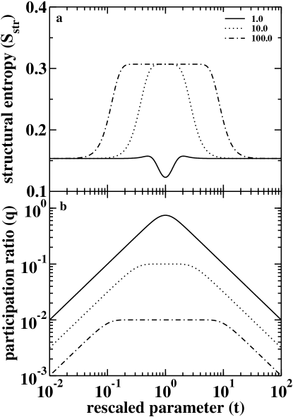
Figure 1: The parameters $S_{str}$ (a, semi-log plot) and $q$ (b, log-log plot) for a Gaussian wave packet as a function of the parameter $t=\alpha/\alpha_{0}$, where $\alpha=L/\sigma$, $L$ is the system size and $\sigma$ is the spreading of the Gaussian. $\alpha_{0}=\sqrt{4\pi\gamma}$. The different curves are parametrized according to $\gamma$, the number of cells within $h$.

where $c_{1}=\sqrt{\pi\gamma/2}$ and $c_{2}=\sqrt{2}c_{1}$. These functions are plotted in Figure 1. At $t=1$ function $q(t)$ is maximal and its value decreases with $\gamma$ as $q(1)\propto\gamma^{-1}$. Only the physically relevant, $\gamma\geq 1$ are plotted. The participation ratio has some very nice, simple behavior, $q^{(\gamma)}(t)\to(t\sqrt{\gamma})^{-1}$ for $t\to\infty$ and $q^{(\gamma)}(t)\to t/\sqrt{\gamma}$ for $t\to 0$. On the other hand in the same limits $S_{str}\to S_{str}^{G}$ independently from $\gamma$ showing that these limits correspond to one dimensional Gaussians in $x$($p$–)directions for $t\to\infty(t\to 0)$. It can also be viewed as if a squeezing parameter made the distribution more coordinate-like (momentum-like) korsch . For intermediate values of $t$, i.e. if $1/\sqrt{\gamma}<t<\sqrt{\gamma}$ with $\gamma\gg 1$ the participation ratio is, $q\approx\gamma^{-1}$ and $S_{str}\approx 2S_{str}^{G}$ indicating that this distribution is a Gaussian in both dimensions, $x$ and $p$. This is the regime where the Husimi–function is a Gaussian in both directions and therefore shows a two-dimensional character. Both curves, $q$ anf $S_{str}$ are symmetrical about $t=1$ on a logarithmic scale of $t$, which is a direct consequence of the geometry of the phase space.

VI Application to disordered systems

Now we calculate Husimi functions of the eigenstates of a disordered one dimensional system. To be more precise we use a tight binding model KM

$$H=\sum_{n}\varepsilon_{n}|n\rangle\langle n|+V\sum_{n}\left(|n\rangle\langle n+1|+|n+1\rangle\langle n|\right)$$ (55)

where $V=1$ is set as the unit of energy and $\varepsilon_{n}$ are random numbers distributed uniformly over the interval $[-W/2,\dots,W/2]$, where $W$ characterizes the strength of disorder. Such a model has been investigated in phase space in Refs. dietmar, and wobst, . The Husimi functions are calculated using Eqs. (40) and (41) from the eigenstates of (55). The participation ratio, $q$, and the structural entropy, $S_{str}$, are calculated according to Eq. (30). We also calculated the Fourier transforms of the eigenstates and obtained smeared distributions according to Eq. (37) both in real and Fourier space. Periodic boundary conditions were considered using $L=512$. The phase space extends over $-L/2\leq x\leq L/2$ and $-\pi<p\leq\pi$, its area is $\Omega=2\pi L$ ($\hbar=1$ and the lower cut-off scale, the lattice spacing is set to unity, $a=1$). Averaging is done over the middle half of the band. In fact, as pointed out by Ref. wobst, , as well, there is no need to average over many realizations of the disordered potential.

Figure 2: Structural entropy, $S_{str}$ (a, semi-log plot) and participation ratio, $q$ (b, log-log plot) as a function of disorder, $W$ in units of $V$, for a one dimensional Anderson model with $L=512$. The squares stand for the states smeared in $x$-representation, the triangles for the states smeared in $p$-representation, the circles are calculated according to Eqs. (50). The dotted lines are simply guides for the eyes. The solid curve corresponds to the values of $S_{str}$ and $q$ for the states in Husimi representation. The circles and the solid curve differ only a little.

When the full Husimi distributions of all states are calculated the computational time grows with $L^{4}$. However, using the approximate relation of Eq. (50), it reduces to roughly $L^{3}$. This is obviously a considerable gain and is comparable to the one achieved in Refs. sugita, ; wobst, .

The results are reported in Fig. 2. Here we have plotted the behavior of parameters (30) versus disorder strength, $W$, and compared to the approximate values obtained using (50). The region where the most important variations of $q$ and $S_{str}$ take place is $W_{1}<W<W_{2}$, where the localization length matches the systems size KM ; vinew , $\lambda\approx L$, i.e. $W_{1}\approx\sqrt{105/L}=0.453$ or its inverse approaches the size of phase space in $p$–direction, $2\pi\lambda\approx 1$, i.e. $W_{2}\approx\sqrt{2\pi 105}=25.68$

Let us analyze the expectations for the limiting cases of $W\to 0$ and $W\to\infty$. It is easy to see that the eigenstates for vanishing disorder are plane waves whose Fourier transform is a Dirac–delta (in fact two, due to the symmetry of the $-p$ and $p$ states). In a ‘smeared’ representation we obtain two Gaussians in $p$-representation. Using Eq. (41) and (30a) we obtain that $q=2/\sqrt{L}$ for the states both in $p$- and Husimi representation. Due to the Gaussian smearing in this limit the structural entropy attains its value of $S_{str}^{G}$ as given in (17). The other limit of $W\to\infty$ is very similar. In that case the eigenstate in $x$-representation has a Dirac–delta character that is smeared to a Gaussian. This results in $q=1/\sqrt{L}$ and again a value of $S_{str}(W)\to S_{str}^{G}$. All these limiting cases are recovered in Fig. 2. The figure shows that the approximation (50) works very well. It is clear that the $x$-, $p$- and Husimi representations are therefore linked very simply.

VII Concluding remarks

In this paper we have presented some important results concerning the applicability of Rényi entropies for the characterization of localization or ergodicity in phase space using the Husimi representation of the quantum states. In fact it has been shown that the differences of Rényi entropies are free from those divergences that would naturally arise due to their application on continuous distributions.

The marginal distributions of the Husimi function are pointed out to have important properties and simple connection to the states in $x$- and $p$-representations.

We have also shown numerically that for disordered systems the limiting distributions of the Husimi function provide most of the information that is needed to describe the Husimi functions themselves. Figure 2 provides a good demonstration of the duality between the $x$- and $p$-representations transparently. A detailed study over the Anderson model in one dimension and the Harper model vinew are left for forthcoming publications.

- (1) K. Życzkowski, J. Phys. A 23, 4427 (1990).
- (2) K. Życzkowski, Physica E (Amsterdam) 9, 583 (2001) and references therein.
- (3) A. Anderson and J.J. Halliwell, Phys. Rev. D48, 2753 (1993).
- (4) B. Mirbach and H-J. Korsch, Ann. Phys., N.Y. 265, 80 (1998); Phys. Rev. Lett. 75, 362 (1995).
- (5) S. Gnutzmann and K. Życzkowski, J. Phys. A: Math. Gen. 34, 10123 (2001).
- (6) A. Sugita and H. Aiba, Phys. Rev. E65, 036205 (2002).
- (7) D. Weinmann, S. Kohler, G.-L. Ingold, and P. Hänggi, Ann. Phys. (Leipzig) 8, SI277 (1999).
- (8) A. Wobst, G.-L. Ingold, P. Hänggi, and D. Weinmann, Eur. Phys. J. B 27, 11 (2002); eprint cond-mat/0303274.
- (9) G.-L. Ingold, A. Wobst, C. Aulbach, P. Hänggi, Eur. Phys. J. B 30, 175 (2002); eprint cond-mat/0212035.
- (10) see e.g. V.K.B. Kota, Phys. Rep. 347, 223 (2001); V. Zelevinsky, B.A. Brown, N. Frazier, and M. Horoi, Phys. Rep. 276, 85 (1996); V.V. Flambaum and F.M. Izrailev, Phys. Rev. E 56, 5144 (1997) and references therein.
- (11) F.M. Izrailev, Phys. Rep. 196, 299 (1990).
- (12) J. Pipek and I. Varga, Phys. Rev. A46, 3148 (1992); Intern. J. of Quantum. Chem. 51, 539 (1994)
- (13) I. Varga, J. Pipek, M. Janssen, and K. Pracz, Europhys. Lett. 36, 437 (1996);
- (14) J. Pipek, I. Varga, and T. Nagy, Intern. J. of Quantum. Chem. 37, 529 (1990); J. Pipek and I. Varga, Intern. J. of Quantum. Chem. 64, 85 (1997).
- (15) I. Varga and J. Pipek, Phys. Rev. B42, 5335 (1990); I. Varga, J. Pipek, and B. Vasvári, Phys. Rev. B46, 4978 (1992); I. Varga and J. Pipek, J. of Phys.:Condens. Matter 6, L115 (1994); I. Varga, Helv. Phys. Acta 68, 68 (1995); I. Varga, and J. Pipek, J. of Phys.:Condens. Matter 10, 305 (1998).
- (16) I. Varga, E. Hofstetter, M. Schreiber, and J. Pipek, Phys. Rev. B52, 7783 (1995); I. Varga, Y. Ono, T. Ohtsuki, and J. Pipek, phys. stat. sol. (b) 205, 373 (1998); M. Metzler and I. Varga, J. Phys. Soc. Japan, 67, 1856 (1998); I. Varga, E. Hofstetter, and J. Pipek, Phys. Rev. Lett. 82, 4683 (1999); J. Pipek, I. Varga and E. Hofstetter, Physica E (Amsterdam) 9, 380 (2001).
- (17) A. Rényi, Rev. Int. Statist. Inst. 33, 1 (1965).
- (18) H.-W. Lee, Phys. Rep. 259, 147 (1995).
- (19) E.P. Wigner, Phys. Rev. 40, 749 (1932).
- (20) L.E. Ballantine: Quantum Mechanics: A Modern Development, (World Scientific, Sigapore, 1999), pp. 414.
- (21) K.E. Cahill and R.J. Glauber, Phys. Rev. 177, 1882 (1969); K. Husimi, Proc. Phys. Math. Soc. Jpn. 22, 264 (1940); it is also known as the Gabor transform: D. Gabor, J. of the Inst. of Elect. Engineers (JIEE) 93, 429 (1946).
- (22) A. Wehrl, Rev. Mod. Phys. 50, 221 (1978).
- (23) H.J. Korsch, C. Müller, and H. Wiescher, J. Phys. A: Math. Gen. 30, L677 (1997).
- (24) B. Kramer and A. MacKinnon, Rep. Prog. Phys. 56, 1469 (1993) and references therein.
- (25) I. Varga, in preparation.