Spinor Bose-Einstein Condensates with Many Vortices

Abstract

Vortex-lattice structures of antiferromagnetic spinor Bose-Einstein condensates with hyperfine spin $F\!=\!1$ are investigated theoretically based on the Ginzburg-Pitaevskii equations near $T_{c}$. The Abrikosov lattice with clear core regions are found never stable at any rotation drive $\Omega$. Instead, each component $\Psi_{i}$ $(i\!=\!0,\pm 1)$ prefers to shift the core locations from the others to realize almost uniform order-parameter amplitude with complicated magnetic-moment configurations. This system is characterized by many competing metastable structures so that quite a variety of vortices may be realized with a small change in external parameters.

Realizations of the Bose-Einstein condensation (BEC) in atomic gases have opened up a novel research field in quantized vortices as created recently with various techniques JILA99 ; ENS00 ; MIT01 ; JILA01 . Especially interesting in these systems are vortices of spinor BEC’s in optically trapped ²³Na Ketterle98 and ⁸⁷Rb Barrett01 , where new physics absent in superconductors Tinkham , ⁴He Donnelly , and ³He Volovik87 ; Thuneberg99 ; Kita01 , may be found.

Theoretical investigations on spinor BEC’s were started by Ohmi and Machida OM98 and Ho Ho98 , followed by detailed studies on vortices with a single circulation quantum Yip99 ; Busch99 ; Volovik00 ; Marzlin00 ; Khawaja01 ; Martikainen01 ; Kurihara01 ; Isoshima01 ; Isoshima02 ; Mizushima02 . However, no calculations have been performed yet on structures in rapid rotation where the trap potential will play a less important role. Indeed, the clear hexagonal-lattice image of magnetically trapped ²³Na MIT01 suggests that predictions on infinite systems are more appropriate for BEC’s with many vortices. Such calculations have been carried out by Ho for the single-component BEC Ho01 and by Mueller and Ho for a two-component BEC Ho02 near the upper critical angular velocity $\Omega_{c2}$ at $T=0$.

The purpose of the present paper is to perform detailed calculations on vortices of $F\!=\!1$ spinor BEC’s in rapid rotation to clarify their essential features. To this end, we focus on the mean-field high-density phase rather than the low-density correlated liquid phase Cooper01 , and use the phenomenological Ginzburg-Pitaevskii (or Ginzburg-Landau) equations near $T_{c}$ GP58 ; GA82 instead of the Gross-Pitaevskii equations at $T=0$. Since fluctuations are small in the present system, this approach will yield quantitatively correct results near $T_{c}$. It should be noted that the corresponding free-energy is formally equivalent to that derived with Ho’s “mean-field quantum Hall regime” near $\Omega_{c2}$ at $T=0$ Ho01 ; Ho02 , so that the results obtained here are also applicable to that region.

Model.— The free-energy density of an $F\!=\!1$ spinor BEC near $T_{c}$ may be expanded with respect to the order parameters $\Psi_{i}$ $(i=0,\pm 1)$ as

$$f=-\alpha\Psi_{i}^{*}\Psi_{i}+\Psi_{i}^{*}\,\frac{\left(-i\hbar\mbox{\boldmath$\nabla$}-M\mbox{\boldmath$\Omega$}\!\times\!{\bf r}\right)^{2}}{2M}\Psi_{i}$$

$$+\frac{\beta_{\rm n}}{2}\Psi_{i}^{*}\Psi_{j}^{*}\Psi_{i}\Psi_{j}+\frac{\beta_{\rm s}}{2}\Psi_{i}^{*}\Psi_{j}^{*}(F_{\mu})_{ik}(F_{\mu})_{jl}\Psi_{k}\Psi_{l}\,.$$ (1)

Here $\alpha$, $\beta_{\rm n}$ , and $\beta_{\rm s}$ are expansion parameters, $F_{\mu}$ $(\mu\!=\!x,y,z)$ denotes the spin operator, $M$ is the particle mass, and summations over repeated indices are implied. The rotation axis $\Omega$ is taken along ${\bf z}$. The quantities $\beta_{\rm n}$ and $\beta_{\rm s}$ are assumed to be constant near $T_{c}$ with $\beta_{\rm n}\!>\!0$, whereas $\alpha$ changes its sign at $T_{c}$ with $\alpha\!>\!0$ for $T\!<\!T_{c}$. To simplify Eq. (1), we measure the length, the energy density, the angular velocity, and the order parameter in units of $\hbar/\sqrt{2M\alpha}$, $\alpha^{2}/\beta_{\rm n}$, $\alpha/\hbar$, and $\alpha/\beta_{\rm n}$, respectively. The corresponding free-energy density is obtained from Eq. (1) by $\alpha\!\rightarrow\!1$, $\beta_{\rm n}\!\rightarrow\!1$, $\hbar^{2}/2M\!\rightarrow\!1$, $M\mbox{\boldmath$\Omega$}\!\rightarrow\!\frac{1}{2}\mbox{\boldmath$\Omega$}$, and $\beta_{\rm s}\!\rightarrow\!g_{\rm s}\!\equiv\!\beta_{\rm s}/\beta_{\rm n}$. It thus takes a simple form with only two parameters $(g_{\rm s},\Omega)$. We then introduce a couple of operators by $a\!\equiv\!\ell(\partial_{x}\!+\!i\partial_{y})/\sqrt{2}$ and $a^{\dagger}\!\equiv\!\ell(-\partial_{x}\!+\!i\partial_{y})/\sqrt{2}$ with $\mbox{\boldmath$\partial$}\!\equiv\!\mbox{\boldmath$\nabla$}-\frac{i}{2}\mbox{\boldmath$\Omega$}\!\times\!{\bf r}$ and $\ell\!\equiv\!1/\sqrt{\Omega}$ which satisfy $aa^{\dagger}\!-\!a^{\dagger}a\!=\!1$. Equation (1) now reads

$$f= \Psi_{i}^{*}[(2a^{\dagger}a\!+\!1)\Omega-1]\Psi_{i}+\frac{1}{2}\Psi_{i}^{*}\Psi_{j}^{*}\Psi_{i}\Psi_{j}$$ (2)

$$+\frac{g_{\rm s}}{2}\Psi_{i}^{*}\Psi_{j}^{*}(F_{\mu})_{ik}(F_{\mu})_{jl}\Psi_{k}\Psi_{l}\,,$$

with $\Omega_{c2}\!=\!1$, and the free-energy is given by

$${\cal F}\equiv\int f({\bf r})\,d{\bf r}\,.$$ (3)

We can find the stable structure for each $(g_{\rm s},\Omega)$ by minimizing ${\cal F}$. We have performed extensive calculations over the whole antiferromagnetic region $g_{\rm s}\!\geq\!0$, where $(\Psi_{1},\Psi_{0},\Psi_{-1})\!=\!{\rm e}^{i\theta}{\cal U}(0,1,0)$ and $f\!=\!\frac{1}{2}$ at $\Omega\!=\!0$ with $\theta$ an arbitrary phase and ${\cal U}$ the spin-space rotation Ho98 .

A major difference from superfluid ³He Kita01 lies in the fact that terms such as $\Psi_{i}^{*}aa\Psi_{j}$ $(i\!\neq\!j)$ are absent, i.e., there are no gradient couplings between different components. Hence $\Omega_{c2}$ is the same for all components, whereas in ³He only a single component becomes finite at $\Omega_{c2}$ to realize the polar state Kita01 . This degenerate feature is what characterizes the present system to bring many competing metastable structures, as seen below.

Method.— We minimize Eq. (3) with the Landau-level-expansion method (LLX) Kita98 ; Kita01 by expanding the order parameters as

$$\Psi_{i}({\bf r})=\sqrt{\cal V}\,\sum_{N=0}^{\infty}\sum_{{\bf q}}c_{N{\bf q}}^{(i)}\,\psi_{N{\bf q}}({\bf r})\,,$$ (4)

with $N$ the Landau-level index, ${\bf q}$ the magnetic Bloch vector, and $\cal V$ the system volume. The basis functions $\{\psi_{N{\bf q}}\}$ are eigenstates of the magnetic translation operator $T_{\bf R}\!\equiv\!\exp[-{\bf R}\cdot(\mbox{\boldmath$\nabla$}+\frac{i}{2}\mbox{\boldmath$\Omega$}\times{\bf r})]$, which can describe periodic vortex structures of all kinds Kita98 . Its explicit expression is given by

$$\psi_{N{\bf q}}({\bf r})\!= \!\!\!\!\!\!\sum_{n=-{\cal N}_{{\rm f}}/2+1}^{{\cal N}_{{\rm f}}/2}\!\!\!\!{\rm e}^{i[q_{y}(y+\ell^{2}q_{x}/2)+na_{1x}(y+\ell^{2}q_{x}-na_{1y}/2)/\ell^{2}]}$$ (5)

$$\times{\rm e}^{-ixy/2\ell^{2}-(x\!-\ell^{2}q_{y}-na_{1x})^{2}/2\ell^{2}}$$

$$\times\sqrt{\frac{2\pi\ell/a_{2}}{2^{N}N!\sqrt{\pi}\,{\cal V}}}H_{\!N}\!\!\left(\!\frac{x\!-\!\ell^{2}q_{y}\!-\!na_{1x}}{\ell}\!\right),$$

with ${\cal N}_{{\rm f}}^{2}$ the number of the circulation quantum $\kappa\!\equiv\!h/M$ in the system, $H_{\!N}$ the Hermite polynomial, and ${\bf a}_{j}$ the basic vectors in the $xy$ plane with ${\bf a}_{2}\!\parallel\!\hat{\bf y}$ and $a_{1x}a_{2}\!=\!2\pi\ell^{2}$. Substituting Eq. (4) into Eq. (3) and carrying out the integration in terms of $(s,t)\!\equiv\!(x/a_{1x},y/a_{2}\!-\!xa_{1y}/a_{1x}a_{2})$, the free energy is transformed into a functional of the expansion coefficients $\{c_{N{\bf q}}^{(i)}\}$, the apex angle $\beta\!\equiv\!\cos^{-1}(a_{1y}/a_{1})$, and the ratio of the two basic vectors $\rho\!\equiv\!a_{2}/a_{1}$ as ${\cal F}\!=\!{\cal F}[\{c_{N{\bf q}}^{(i)}\},\beta,\rho]$. For a given $\Omega$, we directly minimize ${\cal F}/{\cal V}$ with respect to these quantities.

Search for stable structures.— We here sketch our strategy to find stable structures. To this end, we first summarize the basic features of the conventional Abrikosov lattice within the framework of LLX Kita98 : (i) any single ${\bf q}\!=\!{\bf q}_{1}$ suffices, due to the broken translational symmetry of the vortex lattice; (ii) the triangular (square) lattice is made up of $N\!=\!6n$ ($4n$) Landau levels ($n\!=\!0,1,2\cdots$); (iii) more general structures can be described by $N\!=\!2n$ levels, odd $N$’s never mixing up since those bases have finite amplitudes at the cores. This Abrikosov lattice has a single circulation quantum per unit cell.

With multi-component order-parameters, there can be a wide variety of vortices, which may be divided into two categories. We call the first category as “shift-core” states, where core locations are different among the three components with an enlarged unit cell. General structures with $n_{\kappa}$ circulation quanta per unit cell can be described by using $n_{\kappa}$ different ${\bf q}$’s, where the unit cell becomes $n_{\kappa}$ times as large as that of the Abrikosov lattice. For example, structures with two quanta per unit cell are given by choosing $({\bf q}_{1},{\bf q}_{2})\!=\!({\bf 0},\frac{{\bf b}_{1}+{\bf b}_{2}}{2})$, where ${\bf b}_{1}$ and ${\bf b}_{2}$ are reciprocal lattice vectors. This possibility was already considered by Mueller and Ho Ho02 for a two-component system and shown to yield stable structures. It also describes the mixed-twist lattice to be found in ³He Kita01 . The second category may be called “fill-core” states with a single circulation quantum per unit cell (i.e., a single ${\bf q}$ is relevant). Here the cores of the conventional Abrikosov lattice are filled in by some superfluid components using odd-$N$ wavefunctions of Eq. (5). This entry of odd-$N$ Landau levels occurs as a second-order transition below some critical angular velocity smaller than $\Omega_{c2}/3$. It has been shown that the $A$-phase-core vortex in the $B$-phase of superfluid ³He belong to this category Kita01 .

We have carried out an extensive search for stable structures with up to $n_{\kappa}\!=\!9$ circulation quanta per unit cell, including fill-core states. Since we are near $T_{c}$ where normal particles are also present, we have performed the minimization without specifying the value of the magnetic moment $M$ for the superfluid components. However, all the stable states found below have $M\!=\!0$. Each of the three components were expanded as Eq. (4) using $n_{\kappa}$ different ${\bf q}$’s, and the free-energy (3) is minimized with respect to $c_{N{\bf q}}^{(i)}$, $\beta$, and $\rho$ by using Powell’s method NR . To pick out stable structures correctly, we calculated Eq. (3) many times starting from different initial values for $c_{0{\bf q}}^{(i)}$, $\beta$, and $\rho$ given randomly within $0.1\!\leq\!{\rm Re}\hskip 0.85358ptc_{0{\bf q}}^{(i)},\,{\rm Im}\hskip 0.85358ptc_{0{\bf q}}^{(i)}\!\leq\!0.9$, $0.1\pi\!\leq\!\beta\!\leq\!0.5\pi$, and $0.8\!\leq\!\rho\!\leq\!3$, respectively. The state with the lowest energy was thereby identified as the stable structure. The spin quantization axis and an overall phase were fixed conveniently to perform efficient calculations. Thus, any structures obtained from the solutions below with a spin-space rotation and a gauge transformation are also stable.

Instability of Abrikosov lattice.— The present calculations have revealed that the Abrikosov lattice with clear core regions is never stable at any rotation drive $\Omega$ over the entire antiferromagnetic region $g_{\rm s}\!\geq\!0$. Thus, any optical experiments to detect vortices by amplitude reductions are not suitable for the spinor vortices.

The most stable Abrikosov lattice is given by

$$\Psi_{0}({\bf r})=\sqrt{V}\,\sum_{N}c_{N}^{(0)}\psi_{N{\bf q}_{1}}({\bf r})\,,$$ (6)

with $c_{N{\bf q}_{1}}^{(0)}$ real, $N\!=\!6n$, $\beta\!=\!\frac{\pi}{3}$, and $\rho\!=\!1$. Here the antiferromagnetic component $\Psi_{0}$ forms a hexagonal lattice with a single circulation quantum per unit cell. Below some critical velocity $\Omega_{\rm f}$ smaller than $\Omega_{c2}/3$, the core regions start to be filled in by

$$\Psi_{\pm 1}({\bf r})=i\sqrt{V}\,\sum_{N^{\prime}}c_{N^{\prime}}^{(1)}\psi_{N^{\prime}{\bf q}_{1}}({\bf r})\,,$$ (7)

with $N^{\prime}$ odd. The second transition for this odd-Landau-level entry occurs at $\Omega_{\rm f}\!=\!0.1497\Omega_{c2}$ and $0.0938\Omega_{c2}$ for $g_{\rm s}\!=\!0.1$ and $0.3$, respectively.

Figure 1: Spatial variations of (a) the order-parameter amplitude and (b) the magnetic moment along $z$, for the shift-core state (8)-(9) over $|x|,|y|\!\leq\!a_{1}$ at $g_{\rm s}\!=\!0.08$ and $\Omega\!=\!0.95\Omega_{c2}$. The moment is directed along ${\bf z}$.

However, calculations down to $0.0001\Omega_{c2}$ of using $1800$ Landau levels for $g_{\rm s}\!\geq\!0$ have clarified that the above fill-core state carries higher free energy than the following shift-core state with two circulation quanta per unit cell:

$$\Psi_{1}({\bf r})=\sqrt{V}\,\sum_{N}c_{N}\psi_{N{\bf q}_{1}}({\bf r})\,,$$ (8)

$$\Psi_{-1}({\bf r})=\sqrt{V}\,\sum_{N}c_{N}\psi_{N{\bf q}_{2}}({\bf r})\,,$$ (9)

with $c_{N}$ real and common to both, $N\!=\!4n$, $\beta\!=\!\frac{\pi}{2}$, $\rho\!=\!1$, and $({\bf q}_{1},{\bf q}_{2})\!=\!({\bf 0},\frac{{\bf b}_{1}\!+\!{\bf b}_{2}}{2})$. The cores of $\Psi_{\pm 1}({\bf r})$ are shifted from each other by $\frac{1}{2}({\bf a}_{1}\!+\!{\bf a}_{2})$. Figure 1 displays basic features of this shift-core state. The magnetic moment is ordered antiferromagnetically along $z$ axis, and the amplitude is almost uniform taking its maximum at each site where the moment vanishes to form the antiferromagnetic state realized in the uniform state.

Stable structures near $\Omega_{c2}$.— Having seen that the conventional Abrikosov lattice is never favored in the whole antiferromagnetic domain $g_{\rm s}\!\geq\!0$, we now enumerate all the stable structures found near $\Omega_{c2}$ to clarify their essential features. This rapidly rotating domain is especially interesting, because the same free energy also becomes relevant near $\Omega_{c2}$ at $T\!=\!0$, as shown by Ho using a “mean-field quantum Hall regime” Ho01 . Thus, the conclusions obtained here are also applicable to the region at $T\!=\!0$.

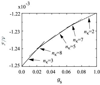
Figure 2: Calculated free energy per unit volume as a function of $g_{\rm s}$ at $\Omega\!=\!0.95\Omega_{c2}$. Five different structures have been found for $g_{\rm s}\!\geq\!0$, and the value of each $n_{\kappa}$ denotes the number of circulation quanta per unit cell for each stable structure.

Figure 2 displays the lowest free energy per unit volume as a function of $g_{\rm s}$ for $\Omega\!=\!0.95\Omega_{c2}$. The value of each $n_{\kappa}$ denotes the number of circulation quanta per unit cell. A special feature to be noted is that these various structures are energetically quite close to each other; for example, the $n_{\kappa}\!=\!8$ state at $g_{\rm s}\!=\!0.02$ is favored over the $n_{\kappa}\!=\!3$ state by a relative free-energy difference of order $10^{-6}$. This fact suggests that we may realize quite a variety of metastable structures by a small change of the boundary conditions, the rotation process, etc.

Details of these structures are summarized as follows.

The $n_{\kappa}\!=\!2$ state of Eqs. (8) and (9) is stable for $g_{\rm s}\geq 0.0671$. We have already seen its basic features above.

The $n_{\kappa}\!=\!3,5,7$ states can be expressed compactly as

$$\Psi_{0}=\sum_{N}\sum_{\nu=1}^{\frac{n_{\kappa}-1}{2}}c_{N{\bf q}_{\nu}}^{(0)}\bigl{(}\,\psi_{N{\bf q}_{\nu}}-{\rm e}^{-2i\frac{\nu}{n_{\kappa}}\pi}\psi_{N{\bf q}_{n_{\kappa}-\nu}}\,\bigr{)}\,,$$ (10)

$$\Psi_{\pm 1}=\sum_{N}\Biggl{[}\,\sum_{\nu=1}^{\frac{n_{\kappa}-1}{2}}c_{N{\bf q}_{\nu}}^{(\pm 1)}\bigl{(}\,\psi_{N{\bf q}_{\nu}}+{\rm e}^{-2i\frac{\nu}{n_{\kappa}}\pi}\psi_{N{\bf q}_{n_{\kappa}-\nu}}\,\bigr{)}$$

$$\hskip 31.29802pt+c_{N{\bf q}_{n_{\kappa}}}^{(\pm 1)}\psi_{N{\bf q}_{n_{\kappa}}}\Biggr{]}\,,$$ (11)

where $N$’s are even and ${\bf q}_{\nu}\!=\!\frac{\nu}{n_{\kappa}}{\bf b}_{1}$. These $n_{\kappa}\!=\!3,5,7$ states are stable for $0\!\leq\!g_{\rm s}\!\leq\!0.0196$, $0.0313\!\leq\!g_{\rm s}\!\leq\!0.0613$, and $0.0613\!\leq\!g_{\rm s}\!\leq\!0.0671$, respectively. Unlike the two component system considered by Mueller and Ho Ho02 where each component is specified by a single-${\bf q}$ basis function, $\Psi_{m}$ here is made up of multiple basis functions $\psi_{N{\bf q}_{\nu}}$ whose cores are shifted from each other by $(\nu/n_{\kappa}){\bf a}_{2}$. Figure 3 displays the basic features of the $n_{\kappa}\!=\!3$ state. The lattice is hexagonal at $g_{\rm s}\!=\!0$, but deforms rapidly as $g_{\rm s}$ increases. The order-parameter amplitude is again almost constant, and the magnetic moment ${\bf M}$ has a complicated structure. These features are common to all the $n_{\kappa}\!\geq\!3$ states discussed here, although no details are presented for the other states. The lattice parameters $(\beta,\rho)$ for $n_{\kappa}\!=5,7$ states are $(0.1311\pi,2.056)$ and $(0.1830\pi,2.609)$ for $g_{\rm s}\!=\!0.05$ and $0.066$, respectively, which change little in each relevant range of stability.

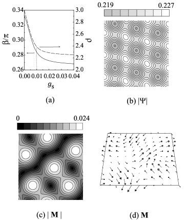
Figure 3: (a) Variations of $\beta/\pi$ and $\rho$ as a function of $g_{\rm s}$ for the $n_{\kappa}\!=\!3$ state at $\Omega\!=\!0.95\Omega_{c2}$. This lattice for $g_{\rm s}\!=\!0$ is hexagonal with $\beta\!=\!\pi/3$ and $\rho\!=\!3$. Figures 2(b)-(d) display, for $g_{\rm s}\!=\!0.01$, spatial variations of (b) the order-parameter amplitude, (c) amplitude of the magnetic moment, and (d) the magnetic moment, over $-3a_{1x}/2<x<3a_{1x}/2$ and $-a_{2}/2<y<a_{2}/2$.

The remaining $n_{\kappa}\!=\!8$ state, stable over $0.0196\!\leq\!g_{\rm s}\!\leq\!0.0313$, is given by

$$\Psi_{0}=\sum_{N}c_{N{\bf q}_{1}}^{(0)}\big{(}\psi_{N{\bf q}_{1}}+\psi_{N{\bf q}_{2}}-\psi_{N{\bf q}_{3}}+i\psi_{N{\bf q}_{4}}\bigr{)}\,,$$ (12)

$$\Psi_{\pm 1}=\sum_{N}\sum_{\nu=5}^{8}c_{N{\bf q}_{\nu}}^{(\pm 1)}\psi_{N{\bf q}_{\nu}}\,,$$ (13)

where ${\bf q}_{1}=\frac{{\bf b}_{1}+{\bf b}_{2}}{2}$, ${\bf q}_{2}={\bf 0}$, ${\bf q}_{3}=\frac{{\bf b}_{1}-{\bf b}_{2}}{4}$, ${\bf q}_{4}=\frac{-{\bf b}_{1}+{\bf b}_{2}}{4}$, ${\bf q}_{5}=\frac{{\bf b}_{1}}{2}$, ${\bf q}_{6}=\frac{{\bf b}_{2}}{2}$, ${\bf q}_{7}=\frac{{\bf b}_{1}+{\bf b}_{2}}{4}$, and ${\bf q}_{8}=\frac{-{\bf b}_{1}-{\bf b}_{2}}{4}$. The parameters $(\beta,\rho)$ at $g_{\rm s}\!=\!0.025$ are $(0.3317\pi,1.049)$, and changes only slightly in the above range of $g_{\rm s}$.

Concluding remarks.—We have performed extensive calculations on antiferromagnetic $F\!=\!1$ spinor vortices in rapid rotation. The conventional Abrikosov lattice is shown never favored. Each stable structure has almost constant order-parameter amplitude and a complicated magnetic-moment configuration, as shown in Figs. 1 and 3, for example. This means that any optical experiments to detect vortices by amplitude reduction will not be suitable for the spinor vortices. Instead, techniques to directly capture spatial magnetic-moment configurations will be required. The system has many metastable structures which are different in the number of circulation quanta per unit cell $n_{\kappa}$, but are quite close to each other energetically. Thus, domains to separate different structures may be produced easily. This degenerate feature is also present within the $(\beta,\rho)$ space of a fixed $n_{\kappa}$, where $\beta$ is the vortex-lattice apex angle and $\rho$ is the length ratio of the two basic vectors. Put it differently, we can deform a stable lattice structure with a tiny cost of energy. These facts indicate that the spinor BEC’s can be a rich source of novel vortices realized with a small change in external parameters.

This research is supported by a Grant-in-Aid for Scientific Research from the Ministry of Education, Culture, Sports, Science, and Technology of Japan.

References

- (1) M. R. Matthews, B. P. Anderson, P. C. Haljan, D. S. Hall, C. E. Wieman, and E. A. Cornell, Phys. Rev. Lett. 83, 2498 (1999).
- (2) K. W. Madison, F. Chevy, W. Wohlleben, and J. Dalibard, Phys. Rev. Lett. 84, 806 (2000).
- (3) J. R. Abo-Shaeer, C. Raman, J. M. Vogels, and W. Ketterle, Science 292, 476 (2001).
- (4) P. C. Haljan, I. Coddington, P. Engels, and E. A. Cornell, Phys. Rev. Lett. 87, 210403 (2001).
- (5) J. Stenger, S. Inouye, D. M. Stamper-Kurn, H.-J. Miesner, A. P. Chikkatur, and W. Ketterle, Nature 369, 345 (1998).
- (6) M. D. Barrett, J. A. Sauer, and M. S. Chapman, Phys. Rev. Lett. 87, 010404 (2001).
- (7) See, e.g., M. Tinkham, Introduction to Superconductivity (McGraw-Hill, New York, 1996).
- (8) R. J. Donnelly, Quantized Vortices in Helium II (Cambridge University Press, Cambridge, 1991).
- (9) M. M. Salomaa and G. E. Volovik, Rev. Mod. Phys. 59, 533 (1987).
- (10) O. V. Lounasmaa and E. Thuneberg, Proc. Nath. Acad. Sci. USA 96, 7760 (1999).
- (11) T. Kita, Phys. Rev. Lett. 86, 834 (2001).
- (12) T. Ohmi and K. Machida, J. Phys. Soc. Jpn. 67, 1822 (1998).
- (13) T.-L. Ho, Phys. Rev. Lett. 81, 742 (1998).
- (14) S. K. Yip, Phys. Rev. Lett. 83, 4677 (1999).
- (15) Th. Busch and J. R. Anglin, Phys. Rev. A60, R2669 (1999).
- (16) U. Leonhardt and G. E. Volovik, JETP Lett. 72, 46 (2000).
- (17) K.-P. Marzlin, W. Zhang, and B. C. Sanders, Phys. Rev. A62, 013602 (2000).
- (18) U. A. Khawaja and H. T. C. Stoof, Nature 411, 918 (2001); Phys. Rev. A64, 043612 (2001).
- (19) J.-P. Martikainen, A. Collin, and K.-A. Suominen, cond-mat/0106301.
- (20) S. Tuchiya and S. Kurihara, J. Phys. Soc. Jpn. 70, 1182 (2001).
- (21) T. Isoshima, K. Machida, and T. Ohmi, J. Phys. Soc. Jpn. 70, 1604 (2001).
- (22) T. Isoshima and K. Machida, cond-mat/0201507.
- (23) T. Mizushima, K. Machida, and T. Kita, cond-mat/0203242.
- (24) T.-L. Ho, Phys. Rev. Lett. 87, 060403 (2001).
- (25) E. J. Mueller and T.-L. Ho, cond-mat/0201051.
- (26) N. R. Cooper, N. K. Wilkin, and J. M. F. Gunn, Phys. Rev. Lett. 87, 120405 (2001).
- (27) V. L. Ginzburg and L. P. Pitaevskii, Zh. Eksp. Teor. Fiz. 34, 1240 (1958) [Sov. Phys. JETP 7, 858 (1958)].
- (28) For a review on this approach, see, V. L. Ginzburg and A. A. Sobyanin, J. Low Temp. Phys. 49, 507 (1982).
- (29) T. Kita, J. Phys. Soc. Jpn. 67, 2067 (1998).
- (30) W. H. Press, S. A. Teukolsky, W. T. Vetterling, and B. P. Flannery, Numerical Recipes in C (Cambridge University Press, Cambridge, 1988).