Superconductivity and Antiferromagnetism
in Three-Dimensional Hubbard model

Abstract

Interplay between antiferromagnetism and superconductivity is studied by using the 3-dimensional nearly half-filled Hubbard model with anisotropic transfer matrices $t_{\rm z}$ and $t_{\perp}$. The phase diagrams are calculated for varying values of the ratio $r_{\rm z}=t_{\rm z}/t_{\perp}$ using the spin fluctuation theory within the fluctuation-exchange approximation. The antiferromagnetic phase around the half-filled electron density expands while the neighboring phase of the anisotropic $d_{x^{2}-y^{2}}$-wave superconductivity shrinks with increasing $r_{\rm z}$. For small $r_{\rm z}$ $T_{\rm c}$ decreases slowly with increasing $r_{\rm z}$. For moderate values of $r_{\rm z}$ we find the second order transition, with lowering temperature, from the $d_{x^{2}-y^{2}}$-wave superconducting phase to a phase where incommensurate SDW coexists with $d_{x^{2}-y^{2}}$-wave superconductivity. Resonance peaks as were discussed previously for 2D superconductors are shown to survive in the $d_{x^{2}-y^{2}}$-wave superconducting phase of 3D systems. Soft components of the incommensurate SDW spin fluctuation mode grow as the coexistent phase is approached.

PACS number:74.25.Dw, 74.20.Mn, 71.10.Fd, 74.70.Tx, 74.72.-h

]

I Introduction

Unconventional superconductivity in strongly correlated electron systems has been one of the central issues in the field of condensed matter physics. It is widely accepted that superconductivity takes place around the antiferromagnetic phase for many strongly correlated systems such as high temperature superconductors [1], $\kappa$-BEDT organic compounds [2, 3], and some of the heavy fermion systems [4, 5]. Naively, superconductivity in these systems is induced by the antiferromagnetic spin fluctuation [6]. In fact, the spin fluctuation theory successfully explains $d_{x^{2}-y^{2}}$-wave superconductivity observed in various quasi two-dimensional systems [7, 8]. Recently, attractive experimental results were presented concerning the relation between antiferromagnetism and superconductivity.

For example, ${\rm CeIn}_{3}$ with a cubic crystal structure exhibits an antiferromagnetic transition with decreasing temperature and it undergoes a superconducting transition under sufficient pressure 25 kbar where the superconducting transition temperature is $T_{\rm c}\approx{0.25}$ K [9]. In relation to this system, a new heavy fermion compound ${\rm CeRhIn}_{5}$ has been discovered recently, in which alternating layers ${\rm CeIn}_{3}$ and ${\rm RhIn}_{2}$ are stacked along the $c$-axis and superconductivity is induced by application of hydrostatic pressure [10]. It is worthwhile to note that superconducting transition temperature $T_{\rm c}\approx{2.1}$ K of this compound is considerably higher than that of ${\rm CeIn}_{3}$ [10]. Adding to this fact, ${\rm CeIrIn}_{5}$ and ${\rm CeCoIn}_{5}$ with the same crystal structure as ${\rm CeRhIn}_{5}$ exhibit superconductivity at ambient pressure [11, 12], so that the crystal structure of ${\rm CeRhIn}_{5}$ is considered to be more favorable for superconductivity than the cubic one. These facts seem to indicate the importance of dimensionality for the occurence of the unconventional superconductivity.

In another recent experiment, NQR measurement under pressure on CeCu₂Si₂ indicated an antiferromagnetic instability in the superconducting phase [13, 14] or possible coexistence between superconductivity and antiferromagnetism. It should also be mentioned that the observation of a neutron resonance peak such as those observed in high-$T_{\rm c}$ cuprates was reported for a heavy electron system UPd₂Al₃ [15, 16, 17, 18, 19]. Thus it is worth while to study the interplay between antiferromagnetism and superconductivity with varying degree of crystal anisotropy or dimensionality using the spin fluctuation theory.

The effect of dimensionality on spin fluctuation-mediated superconductivity was studied previously both with the use of phenomenological models for spin fluctuations [20, 21] and from fully microscopic calculations based on the Hubbard model [22]. In these studies comparisons were made between two ideal cases with simple square and cubic lattices. In view of recent experiments it seems important to study the effect of crystal anisotropy interpolating between ideal 2D and 3D systems.

In this paper, we discuss the phase diagram of the three dimensional anisotropic Hubbard model using the fluctuation exchange (FLEX) approximation [23, 24, 25, 26]. The crystal anisotropy or dimensionality is controlled by a parameter $r_{z}$ which is the ratio of the out-of-plane hopping integral to the in-plane one. Notice that cases of $r_{z}=0$ and $r_{z}=1$ correspond to the square lattice and the cubic lattice, respectively. We restrict ourselves near the half-filled electron density and $0<r_{z}<1$. Our results are summarized in following four features. (1) With increasing $r_{\rm z}$ the area of the magnetic phase in the phase diagram tends to expand while that of the $d_{x^{2}-y^{2}}$-wave superconducting phase shrinks. (2) For a moderate value of $r_{\rm z}$ the $d_{x^{2}-y^{2}}$-wave superconducting phase undergoes a second order phase transition into a coexistent phase between $d_{x^{2}-y^{2}}$-wave superconductivity and incommensurate spin density wave (ICSDW). (3) For the same value of $r_{\rm z}$ the spin fluctuation frequency spectra show a resonance peak or ridge around the antiferromagnetic wave vector, similarly to the one studied previously for 2-dimensional systems. The latter has been interpreted as the spin-excitonic collective mode and was assigned to the neutron resonance peaks observed in Y- and Bi-based high-$T_{\rm c}$ cuprates. (4) Low frequency components of the spin fluctuation spectrum corresponding to the ICSDW ordering vector grow significantly as the phase transition point is approached.

In what follows we discuss the model Hamiltonian and approximation procedure in Sec. II and the results of calculation in Sec. III. Sec. IV is devoted for general discussion and summary.

II Model and FLEX approximation

A Model Hamiltonian

The model Hamiltonian we use here is;

$$H=\sum_{{\bf k},\sigma}\epsilon_{{\bf k}}a_{{\bf k}\sigma}^{\dagger}a_{{\bf k}\sigma}+U\sum_{i}n_{i\uparrow}n_{i\downarrow},$$ (1)

where $a_{{\bf k}\sigma}^{\dagger}$ is the creation operator for a quasi-particle with momentum ${\bf k}$ and spin $\sigma$, $U$ is the on-site Coulomb energy, $n_{i\sigma}$ is the number operator for a quasi-particle with spin $\sigma$ at $i$-site. $\epsilon_{{\bf k}}$ is the energy dispersion of the quasi-particle given by

$$\epsilon_{{\bf k}}= -2t(\cos{k_{x}}+\cos{k_{y}})+4t^{\prime}\cos{k_{x}}\cos{k_{y}}$$ (3)

$$-2t\hskip 2.84526ptr_{z}\cos{k_{z}}+4t^{\prime}r_{z}\cos{k_{z}}(\cos{k_{x}}+\cos{k_{y}})$$

where $t$ and $t^{\prime}$ are the nearest-neighbor and the next nearest-neighbor hopping integrals, respectively. Hereafter, $t$ is used as the unit of energy. Also, we introduce a parameter $r_{z}$ describing the anisotropy along $z$-axis where $r_{z}=0$ corresponds to the square lattice, and $r_{z}=1$ to the cubic lattice. Although the value of the anisotropy parameter for the next nearest-neighbor hopping should be generally different from that for the nearest-neighbor, we use the same value for them since no essential difference will appear by definite distinction between them. The variation of the phase diagram with this anisotropy is studied using the Green’s function method.

B FLEX Approximation

When the interaction constant $U$ is equal to zero, the one-particle Green’s function of the quasi-particle at temperature $T$ is given by

$$G^{(0)}({\bf k},{\rm i}\omega_{n})=\frac{1}{{\rm i}\omega_{n}-\epsilon_{\bf k}+\mu}$$ (4)

where $\omega_{n}=(2n+1)\pi T$ is the Fermion Matsubara frequency and $\mu$ is the chemical potential.

For the three dimensional system with $U\neq 0$, various ordered states appear at respective transition temperature below which features of the system is described by corresponding order parameters, and anomalous Green’s functions. In order to study the interplay between magnetism and superconductivity, we wish to construct the phase diagram of this model calculating the magnetic and superconducting transition points. In the FLEX approximation the superconducting $T_{\rm c}$ is calculated within a mean field level while the magnetic susceptibility is renormalized self-consistently and thus there is no Neel temperature $T_{\rm N}$ for 2D-systems. Here the finite value of $r_{\rm z}$ or 3D-character makes it possible to find magnetic transition point $T_{\rm N}$ from the divergence of $\chi_{Q}$.

The Dyson-Gor’kov equations for the Green’s functions and the anomalous Green’s functions are given by

$$G(k)=G^{(0)}(k)+G^{(0)}(k)\Sigma^{(1)}(k)G(k)$$ (5)

$$\hskip 68.2866pt-G^{(0)}(k)\Sigma^{(2)}(k)F^{\dagger}(k)$$ (6)

$$F^{\dagger}(k)=G^{(0)}(-k)\Sigma^{(1)}(-k)F^{\dagger}(k)$$ (7)

$$\hskip 28.45274pt+G^{(0)}(-k)\Sigma^{(2)}(-k)G(k)$$ (8)

where the abbreviation $k\equiv({\bf k},{\rm i}\omega_{n})$ is used and $G(k)$ is Green’s function for $U\neq 0$. $F^{\dagger}(k)$ is anomalous Green’s function to describe the superconducting phase. The self-energies $\Sigma^{(1)}(k)$ and $\Sigma^{(2)}(k)$ are given within the FLEX approximation as follows [23, 24, 25, 26]:

$$\Sigma^{(1)}(k)=\sum_{q}V_{\rm eff}(q)G(k-q),$$ (9)

$$\Sigma^{(2)}(k)=-\sum_{q}V_{\rm sing}(q)F^{\dagger}(k-q),$$ (10)

$$V_{\rm eff}(q)=U^{2}[\frac{3}{2}\chi^{\rm s}(q)+\frac{1}{2}\chi^{\rm c}(q)-\frac{1}{2}\{\overline{\chi}^{\rm s}(q)+\overline{\chi}^{\rm c}(q)\}]$$ (11)

$$V_{\rm sing}(q)=U^{2}[\frac{3}{2}\chi^{\rm s}(q)-\frac{1}{2}\chi^{\rm c}(q)-\frac{1}{2}\{\overline{\chi}^{\rm s}(q)-\overline{\chi}^{\rm c}(q)\}]$$ (12)

with

$$\chi^{\rm s}(q)=\frac{\overline{\chi}^{\rm s}(q)}{1-U\overline{\chi}^{\rm s}(q)},\hskip 14.22636pt\chi^{\rm c}(q)=\frac{\overline{\chi}^{\rm c}(q)}{1+U\overline{\chi}^{\rm c}(q)},$$ (13)

$$\overline{\chi}^{\rm s(c)}(q)=-\sum_{k}[G(k+q)G(k){\pm}F^{\dagger}(k+q)F^{\dagger}(k)]$$ (14)

where $q\equiv({\bf q},{\rm i}\Omega_{n})$ and $\Omega_{n}=2n\pi T$ is the Boson Matsubara frequency. Also, $\sum_{k}\equiv\frac{T}{N_{0}}\sum_{\bf k}\sum_{n}$ and $N_{0}$ is the number of sites. $\chi^{\rm s(c)}(q)$ and $\overline{\chi}^{\rm s(c)}(q)$ are spin (charge) susceptibility and its irreducible part, respectively. Due to the analytical continuation of $\chi^{\rm s(c)}(q)$ from the imaginary axis to the real axis, spectrum of spin (charge) fluctuations is provided.

For the purpose of calculating $T_{\rm c}$ we linearize this Dyson-Gor’kov equations with respect to $F^{\dagger}(k)$ or $\Sigma^{(2)}(k)$ as follows:

$$G(k)=\frac{1}{G^{(0)}(k)^{-1}-\Sigma^{(1)}(k)},$$ (15)

$$F^{\dagger}(k)=|G(k)|^{2}\Sigma^{(2)}(-k)$$ (16)

where the normal self-energy $\Sigma^{(1)}(k)$ in eq. (12) corresponds to that of the normal state. The transition temperature for superconductivity is determined as the temperature below which the linearized equation for $\Sigma^{(2)}(k)$ has a non-trivial solution. The linearized equation is given as

$$\Sigma^{(2)}(k)=-\sum_{p}[V_{\rm sing}(k-p)|G(p)|^{2}]_{\Sigma^{(2)}\rightarrow 0}\Sigma^{(2)}(p)$$ (17)

where $T_{\rm c}$ is obtained by the temperature at which the maximum eigenvalue becomes unity. Note that the superconducting order parameter has the same symmetry as $\Sigma^{(2)}(k)$.

C Details of Numerical Calculation

The FLEX calculation is numerically carried out for each value of $r_{z}$ at fixed parameter values of $t^{\prime}=0.2$ and $U=6$. All summations involved in the above self-consistent equations are calculated using FFT algorism for the ${\bf k}$-space with $16\times 16\times 16$ meshes in the first Brillouin zone and Matsubara frequency sums with sufficiently large cutoff-frequency $\omega_{\rm c}=36$. Although the lattice size seems to be relatively small, it is considered that the obtained results are quantitatively modified but does not qualitatively change with magnification of the system size. When relative error of the self-energy for all ${\bf k}$ and $\omega_{n}$ becomes smaller than $10^{-6}$, it is assumed that the solution is obtained for the self-consistent equations mentioned above. The second-order magnetic phase transition is given by

$$U\overline{\chi}^{\rm s}({\bf q},{\rm i}\Omega_{n}=0)=1$$ (18)

where a spin susceptibility ${\chi}^{\rm s}({\bf q},{\rm i}\Omega_{n}=0)$ diverges. Since numerical calculation can not treat any divergences, we always adopt following condition as the condition for the magnetic transition

$$U\overline{\chi}^{\rm s}({\bf q},{\rm i}\Omega_{n}=0)=1-\epsilon$$ (19)

where $\epsilon=0.002$ is used throughout these calculations; $U\overline{\chi}^{\rm s}({\bf q},0)\approx 1$[27]. It should be noted that slight modification for the value of $\epsilon>0$ does not bring about qualitative changes for our results. The superconducting transition tempertures are determined by solving the gap equation (14) obtained within FLEX approximation. The analytical continuations of $\chi^{\rm s(c)}(q)$ to the real axis are carried out by using Pad$\acute{\rm e}$ approximants.

III Calculated Results

A Phase Diagrams

In this section, the results of FLEX calculation for the model mentioned above are shown. We begin by examining variation with the anisotropy parameter $r_{z}$ of the phase diagram in temperature $T$ vs hole-doping concentration $(1-n)$ space, where $n$ is the electron density per site. The calculated phase diagrams are shown in the Fig. 1; 1(a), 1(b), 1(c), 1(d), and 1(e) are the results for $r_{z}=0.1$, 0.2, 0.4, 0.6, and 0.8, respectively. Each symbol used in these figures has the following meaning; closed circles show the transition to the superconducting phase with $B_{\rm 1g}$-symmetry and open circles, open squares, open diamonds, and open triangles correspond to the magnetic transition with the SDW wave vector of ${\bf Q}=(\pi,\pi,\pi)$, ${\bf Q}_{1}=(0.88\pi,\pi,\pi)$, ${\bf Q}_{2}=(0.75\pi,\pi,\pi)$, and ${\bf Q}_{3}=(0.88\pi,0.88\pi,\pi)$, respectively. Also, closed squares in Fig. 1(b) and closed diamonds in Fig. 1(c) show the second-order magnetic transition between the $d_{x^{2}-y^{2}}$-wave superconducting phase and the coexistent phase with the SDW wave vector of ${\bf Q}_{1}$ and ${\bf Q}_{2}$, respectively. It should be noted that all of these phase transitions are of the second-order. Adding to these phase transition points, symbols of plus, times, sharp, and asterisk in Fig. 1 correspond to the crossover temperatures at which the peak position of $\chi^{\rm s}({\bf q},0)$ changes from ${\bf Q}$ to ${\bf Q}_{1}$, ${\bf Q}_{1}$ to ${\bf Q}_{2}$, ${\bf Q}_{1}$ to ${\bf Q}_{3}$, and ${\bf Q}_{3}$ to ${\bf Q}_{2}$, respectively. For example, in the case of $n=0.85$ in Fig. 1(b), the peak position of $\chi^{\rm s}({\bf q},0)$ changes from ${\bf Q}$ to ${\bf Q}_{1}$ with the decrease of temperature, and then $d_{x^{2}-y^{2}}$-wave superconductivity appears. For more detailed change in the peak position we need more detailed calculation using smaller mesh in the ${\bf q}$-space. In the systems with nearly half-filled density, the peak of $\chi^{\rm s}({\bf q},0)$ always appear at the commensurate position ${\bf q=Q}$ for moderately high temperature region as shown in Fig. 1. This fact is consistent with the results of previous calculations for 2D systems [24, 25, 26].

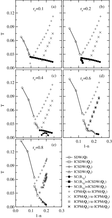
FIG. 1.: $T$ vs $1-n$ phase diagrams for (a) $r_{z}=0.1$, (b) $r_{z}=0.2$, (c) $r_{z}=0.4$, (d) $r_{z}=0.6$, and (e) $r_{z}=0.8$. The abbreviations used here have following meaning; SDW(${\bf Q}$): commensurate SDW phase, ICSDW(${\bf Q}_{n}$): incommensurate SDW phase with wave vector ${\bf Q}_{n}$, SC($B_{\rm 1g}$): $d_{x^{2}-y^{2}}$-wave superconducting phase, CPM(${\bf Q}$): paramagnetic phase with commensurate peak for $\chi^{\rm s}({\bf q},0)$, and ICPM(${\bf Q}_{n}$): paramagnetic phase with incommensurate peak at ${\bf q}={\bf Q}_{n}$. Also, the meanings of all symbols is explained in text.

One of the important results we find from Fig. 1 is the gradual suppression of the $d_{x^{2}-y^{2}}$-wave superconducting phase with increasing $r_{\rm z}$ or increasing three dimensionality in contrast to the gradual expansion of the antiferromagnetic phase. For $r_{\rm z}=0.8$ the $d_{x^{2}-y^{2}}$-wave superconducting phase is very much suppressed in accord with the previous calculation for the simple cubic lattice [22]. An interesting result here is that with increasing $r_{\rm z}$ from zero or 2D limit $T_{\rm c}$ first decreases but slowly. Even for $r_{\rm z}=0.4$, with substantial 3D character, $T_{\rm c}$ is not much reduced from the 2D value. Explicit plots are found in the inset of Fig. 2. For still increasing value of $r_{\rm z}$, $T_{\rm c}$ decreases rapidly. These results indicate that materials with layered structure such as cuprates and Ce-115 heavy fermion compounds are quite favorable for the appearance of $d_{x^{2}-y^{2}}$-wave superconductivity.

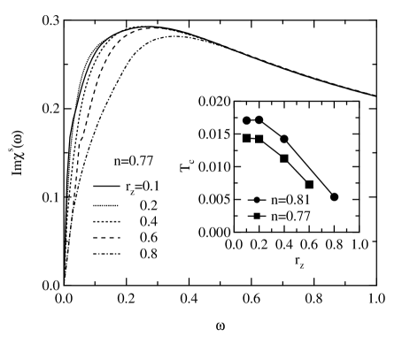
FIG. 2.: Calculated results of $\omega$-dependences of ${\rm Im}\chi^{\rm s}(\omega)$ for respective $r_{z}$-value at fixed electron density $n=0.77$ where temperature is set just above $T_{\rm c}$ except for the case of $r_{z}=0.8$ for which $T=0.005$. Inset: $r_{z}$-dependence of $T_{\rm c}$ at fixed electron densities $n=0.81$ and $n=0.77$.

Another important result is the possible coexistent phase between $d_{x^{2}-y^{2}}$-wave superconductivity and ICSDW as seen in Fig. 1(b) and 1(c). It should be noted that the SDW ordering vectors ${\bf Q}_{1}$ and ${\bf Q}_{2}$ in 1(b) and 1(c) are the same as the ones corresponding to the peak positions of $\chi^{\rm s}({\bf q},0)$ just above the superconducting transition temperature. Considering this new feature of the phase diagram it seems worth while to look at the dynamical susceptibility around the coexistent phase. It is also interesting to see if the spin-excitonic collective modes as were found in 2D systems persist for 3D systems and give simultaneous explanations for the resonance peaks observed in high-$T_{\rm c}$ cuprates and in certain heavy electron superconductor. These problems will be discussed in the following subsection.

B Spectra of Spin Fluctuations

In order to get some idea about the possible reason for the reduction of $T_{\rm c}$ with increasing $r_{\rm z}$ we have calculated the ${\bf q}$-integrated imaginary part of the dynamical susceptibility

$${\rm Im}\chi^{\rm s}(\omega)=\frac{1}{N_{0}}\sum_{\bf q}{\rm Im}\chi^{\rm s}({\bf q},\omega+{\rm i}\delta)$$ (20)

for varying values of $r_{\rm z}$ at a fixed electron density 0.77 and just above $T_{\rm c}$. The results are shown in Fig. 2. The $r_{\rm z}$-dependence of $T_{\rm c}$ is also shown in the inset for $n=0.77$ and $n=0.81$.

We see from this figure that with increasing $r_{\rm z}$ the relatively low frequency components (but much higher than the order of $T_{\rm c}$) decreases while the higher frequency side of the spectrum is fixed. This decrease of the intensity of spin fluctuation is particularly significant for $r_{\rm z}>0.4$ and is considered to be responsible for the reduction of $T_{\rm c}$.

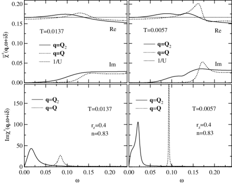
FIG. 3.: Calculated results of $\omega$-dependences of (upper) $\overline{\chi}^{\rm s}({\bf q},\omega+{\rm i}\delta)$ and (lower) Im$\chi^{\rm s}({\bf q},\omega+{\rm i}\delta)$ for ${\bf q}={\bf Q}_{2}$(solid line) and ${\bf q}={\bf Q}$ (dotted line) at two temperatures (left) $T=0.0137$ and (right) $T=0.0057$ below $T_{\rm c}=0.0157$ where parameter set ($r_{z},n$) is fixed to (0.4, 0.83).

We next discuss the behaviors of the predominant components of the dynamical susceptibility in the situations where the phase transition between the $d_{x^{2}-y^{2}}$-wave superconducting and the coexistent phases takes place as seen in Fig. 1(b) and 1(c). As a representative example we choose the parameter set $(r_{\rm z},n)=(0.4,0.83)$ in Fig. 1(c). We show in Fig. 3 the spin fluctuation spectra below $T_{\rm c}$ for the antiferromagnetic component with the wave vector $\bf Q$ and for the SDW components with the incommensurate wave vector ${\bf Q}_{2}$. The upper and lower pannels show the calculated results of the $\omega$-dependences of the irreducible spin susceptibilities and the imaginary part of the spin susceptibilities, respectively, where these quantities have following relation according to equation (10)

$${\rm Im}\chi^{\rm s}({\bf q},\omega+{\rm i}\delta)$$ (21)

$$=\frac{{\rm Im}\overline{\chi}^{\rm s}({\bf q},\omega+{\rm i}\delta)}{[1-U{\rm Re}\overline{\chi}^{\rm s}({\bf q},\omega+{\rm i}\delta)]^{2}+[U{\rm Im}\overline{\chi}^{\rm s}({\bf q},\omega+{\rm i}\delta)]^{2}}.$$ (22)

We first note that the intensity of Im$\chi^{\rm s}({\bf Q},\omega+{\rm i}\delta)$ around $\omega=0.08$ develops strongly with decreasing temperature. As proposed in previous papers [28, 29, 30], it is considered that this peak corresponds to the spin-excitonic collective mode within the $d_{x^{2}-y^{2}}$-wave superconducting phase taking into account that the excitation energy for this mode is less than the superconducting gap $2\Delta\approx 0.17$ estimated from the peak-position of Im$\overline{\chi}^{\rm s}({\bf Q},\omega+{\rm i}\delta)$. Noting that relatively large value of $r_{z}$ is used in Fig. 3, it is considered that such a collective mode is not specific to 2D systems but appears more generally in 3D systems with the $d_{x^{2}-y^{2}}$-wave superconducting phase induced by the antiferromagnetic spin fluctuation. Thus, although this feature is discussed in relation with the 41meV resonance peak observed in Y- and Bi-based cuprates [31, 32], it is expected that such a collective mode within the $d_{x^{2}-y^{2}}$-wave superconducting state should be seen in another unconventional superconductors such as UPd₂Al₃ [15, 16, 17, 18, 19]. As is seen in Fig. 3, the spectrum of the spin fluctuation with the wave vector ${\bf Q}_{2}$ also exhibits such a collective mode around $\omega=0.02$. In addition to this, a new excitation appears with decreasing temperature as a shoulder of ${\rm Im}\chi^{\rm s}({\bf Q}_{2},{\omega}+{\rm i}\delta)$ near $\omega=0$ . This behavior is considered to be associated with the instability of the ICSDW mode ${\bf Q}_{2}$ at the second order transition point to the coexistent phase. Recent higher-resolution inelastic neutron scattering experiment shows that the shoulder on low excitation energy is observed at the incommensurate position below $T_{\rm c}$ in the under-doped high-$T_{\rm c}$ cuprates[33]. Such an experimental data may be related with the behavior shown in Fig. 3.

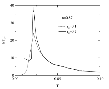
FIG. 4.: Calculated results of $T$-dependences of $1/T_{1}T$ for $r_{z}=0.1$ (dotted line) and $r_{z}=0.2$ (solid line) at fixed electron density $n=0.87$ where their $d_{x^{2}-y^{2}}$-wave superconducting transition temperatures are almost same as seen in Fig. 1.

These low energy excitations are considered to affect various physical quantities, especially, the nuclear spin-lattice relaxation rate $1/T_{1}$ which is expressed as

$$\frac{1}{T_{1}T}\approx\sum_{\bf q}\frac{{\rm Im}\chi^{\rm s}({\bf q},\omega+{\rm i}\delta)}{\omega}|_{\omega\rightarrow 0}$$ (23)

where the hyperfine coupling constant is assumed to be unity. It is well known that $1/T_{1}T$ exhibits the $T^{2}$-law for the $d_{x^{2}-y^{2}}$-wave superconductor due to the existence of line nodes as in the high-$T_{\rm c}$ cuprates. But, it is expected that if this type of excitations exist as seen for ${\rm Im}\chi^{\rm s}({\bf Q}_{2},{\omega}+{\rm i}\delta)$ in Fig. 3, $1/T_{1}T$ should show an upturn below $T_{\rm c}$ as shown in Fig. 4. In fact, such a behavior is recently reported for ${\rm CeCu}_{2}{\rm Si}_{2}$ [13, 14] where it is known that the unconventional superconductiviting transition takes place at low temperature and the magnetic phase, so-called $A$-phase, exists under the magnetic field.

IV Discussion and Summary

Since the second-order phase transition accompanies some symmetry-breaking, it is instrucitve to discuss phase transitions considering the symmetry for the respective phase in those phase diagrams. As wellknown, the Hubbard model shown in eq. (1) has $D_{4h}{\times}SU(2){\times}\Theta{\times}U(1)$-symmetry where $D_{4h}$ is tetragonal point group of the system, $SU(2)$ rotational invariance in the spin-space, $\Theta$ time-reversal symmetry, and $U(1)$ gauge symmetry. When the antiferromagnetic or SDW transition takes place with the magnetic moment along $z$-axis, the $SU(2)$ rotational invariance is broken and $D_{4h}{\times}\Theta$ reduces to its subgroup $\overline{D}_{4h}$, so that the symmetry of the system lowers to $\overline{D}_{4h}{\times}U(1)$ where $\overline{G}$ is a magnetic point group which includes some group elements for $G$’s typical element $R$ to couple with the time-reversal operator $\theta$. Also, the $d_{x^{2}-y^{2}}$-wave superconducting transition (belonging to $B_{\rm 1g}$ irreducible representation) breaks $U(1)$ gauge symmetry and $\pi/2$-rotational invariance, so that the symmetry of this phase becomes $D_{2h}{\times}SU(2){\times}\Theta$.

Of course, the first-order phase transition between SDW and $d_{x^{2}-y^{2}}$-wave superconducting phases is possible where a group of one phase is not a subgroup of the other. Noting that no magnetic transition takes place in the $d_{x^{2}-y^{2}}$-wave superconducting phase in Fig. 1(a), it seems that such first-order phase transitions take place between SDW and $d_{x^{2}-y^{2}}$-wave superconducting phases as schematically shown in Fig. 5(a). On the other hand, the second-order phase transitions are expected between the coexistent phase and the ICSDW and $d_{x^{2}-y^{2}}$-wave superconducting phases because the group $\overline{D}_{2h}$ of the coexistent phase is a subgroup of both of the other two phases as seen in Fig. 5(b). It seems that Fig. 1(b) corresponds to such a case. In Fig. 1(c), it seems that the transition between the $d_{x^{2}-y^{2}}$-wave superconducting phase and the coexistent phase is of the second-order while the first-order phase transition is expected between the $d_{x^{2}-y^{2}}$-wave superconducting and the ICSDW phases, as shown in Fig. 5(c).

Finally, it may be worth while to make a comment on the spin excitations in the coexistent phase. In view of the symmetry of the coexistent phase we may naturally expect to have a Goldstone or zero frequecncy spin wave mode which recovers the broken $SU(2)$-symmetry. We have seen in Fig. 3 that the soft component as a shoulder of the spin excitonic collective mode at the ICSDW wave vector ${\bf Q}_{2}$ grows while the main peak position is kept finite as the coexistent phase is approached. The softening component may be regarded as a precursor to the appearance of the Goldstone mode. Thus in the coexistent phase we may generally expect to have two types of spin excitation modes, the spin excitonic collective mode associated with the superconducting gap and the spin wave mode associated with antiferromagnetism (including SDW). When $T_{\rm N}$ is substantially higher than $T_{\rm c}$, however, the appearance of the former mode itself seems to be dubious from consideration of the possible gap structure. It should be an interesting future subject to study the dispersions and the ranges of appearance of these modes.

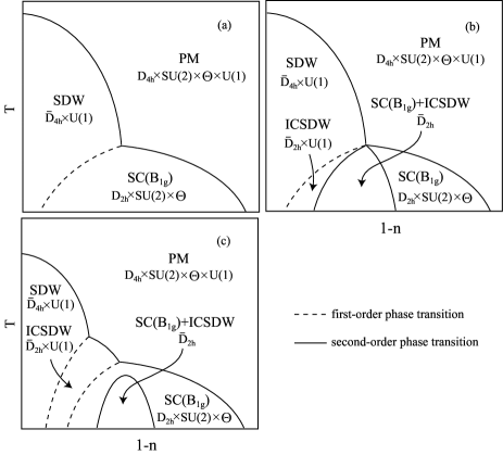
FIG. 5.: Schematic phase diagrams corresponding to Fig. 1(a), 1(b), and 1(c). The left edges of these figures correspond to half filled density. Here, PM, SDW, ICSDW, and SC($B_{\rm 1g}$) stand for the paramagnetic metal, SDW, incommensurate SDW, and $d_{x^{2}-y^{2}}$-wave superconducting phase, respectively. In SC($B_{\rm 1g}$)+ICSDW phase, $d_{x^{2}-y^{2}}$-wave superconductivity and ICSDW coexist. Also, the symmetry of respective phase is written in order to discuss what kind of symmetry is broken.

In summary, the phase diagram of the three-dimensional anisotropic Hubbard model with varying ratio $r_{\rm z}$ of the transfer matrices along z-axis and in xy-plane is calculated by using the spin fluctuation theory within the FLEX approximation. The results are summarized as follows: (1) For small $r_{\rm z}$ or nearly 2-dimensional case we have an antiferromagnetic phase around the half-filled electron density and a $d_{x^{2}-y^{2}}$-wave superconducting phase neighboring to it. With increasing $r_{\rm z}$ the antiferromagnetic phase tends to expand while the $d_{x^{2}-y^{2}}$-wave superconducting phase shrinks. For relatively small values of $r_{\rm z}$, however, this trend is weak and the superconducting transition temperature $T_{\rm c}$ decreases slowly with increasing $r_{\rm z}$. As $r_{\rm z}$ approaches 1, $T_{\rm c}$ decreases rapidly. This behavior of $T_{\rm c}$ seems to be related with the reduction in the ${\bf q}$-integrated intensity of the spin fluctuation spectrum mainly in relatively low frequency (but much higher than the order of $T_{\rm c}$) side. (2) For a moderate value of $r_{\rm z}$ the $d_{x^{2}-y^{2}}$-wave superconducting phase undergoes a second-order transition, with decreasing temperature, into a phase where incommensurate spin density wave (ICSDW) coexists with $d_{x^{2}-y^{2}}$-wave superconductivity. (3) For the same value of $r_{\rm z}$ the spin fluctuation frequency spectra show a resonance peak or ridge around the antiferromagnetic wave vector, similarly to the one studied previously for two-dimensional systems. These spin-excitonic collective modes are considered to explain the neutron resonance peaks observed in Y- and Bi-based high-$T_{\rm c}$ cuprates and in a heavy Fermion system UPd₂Al₃. (4) The low frequency components of the ICSDW mode of spin fluctuations grow significantly as the transition point between the $d_{x^{2}-y^{2}}$-wave superconducting and coexistent phases is approached.

Recently, in order to discuss the effect of orbital degeneracy to superconductivity, the weak coupling theory is developed where the orbital fluctuation plays an important role as well as spin fluctuation [34, 35]. Since any fluctuations should be treated dynamically, it is desireble to construct the strong coupling theory including the orbital degree of freedom.

REFERENCES

- [1] J. G. Bednorz and K. A. Mller, Z. Phys. B 64, 189 (1986).
- [2] D. Jérome and H. J. Schulz, Adv. Phys. 31, 299 (1982).
- [3] T. Ishiguro, K. Yamaji, and G. Saito, Organic Superconductors, 2nd ed. (Springer-Verlag, Berlin, 1998).
- [4] F. Steglich, J. Aarts, C. D. Bredl, W. Lieke, D. Meschede, W. Franz, and H. Schfer, Phys. Rev. Lett. 43, 1892 (1979).
- [5] C. Geibel, C. Schank, S. Thies, H. Kitazawa, C. D. Bredl, A. Bhm, M. Rau, A. Grauel, R. Caspary, R. Helfrich, U. Ahlheim, G. Weber, and F. Steglich, Z. Phys. B 84, 1 (1991).
- [6] N. D. Mathur, F. M. Grosche, S. R. Julian, I. R. Walker, D. M. Freye, R. K. W. Haselwimmer, and G. G. Lonzarich, Nature 394, 39 (1998).
- [7] D. J. Scalapino, Phys. Rep. 250, 329 (1995).
- [8] T. Moriya and K. Ueda, Adv. Phys. 49, 555 (2000).
- [9] I. R. Walker, F. M. Grosche, D. M. Freye, and G. G. Lonzarich, Physica C 282-287, 303 (1997).
- [10] H. Hegger, C. Petrovic, E. G. Moshopoulou, M. F. Hundley, J. L. Sarrao, Z. Fisk, and J. D. Thompson, Phys. Rev. Lett. 84, 4986 (2000).
- [11] C. Petrovic, R. Movshovich, M. Jaime, P. G. Pagliuso, M. F. Hundley, J. L. Sarrao, Z. Fisk, and J. D. Thompson, Europhys. Lett. 53, 354 (2001).
- [12] C. Petrovic, P. G. Pagliuso, M. F. Hundley, R. Movshovich, J. L. Sarrao, J. D. Thompson, Z. Fisk, and P. Monthoux, J. Phys.: Condens. Matter 13, L337 (2001).
- [13] K. Ishida, Y. Kawasaki, K. Tabuchi, K. Kashima, Y. Kitaoka, K. Asayama, C. Geibel, and F. Steglich, Phys. Rev. Lett. 82, 5353 (1999).
- [14] Y. Kawasaki, K. Ishida, T. Mito, C. Thessieu, G.-q. Zheng, Y. Kitaoka, C. Geibel, and F. Steglich, Phys. Rev. B63, 140501(R) (2001).
- [15] N. Metoki, Y. Haga, Y. Koike, N. Aso, and Y. nuki, J. Phys. Soc. Jpn. 66, 2560 (1997).
- [16] N. Metoki, Y. Haga, Y. Koike, and Y. nuki, Phys. Rev. Lett. 80, 5417 (1998).
- [17] N. Bernhoeft, N. Sato, B. Roessli, N. Aso, A. Hiess, G. H. Lander, Y. Endoh, and T. Komatsubara, Phys. Rev. Lett. 81, 4244 (1998).
- [18] N. Bernhoeft, Eur. Phys. J. B 13, 685 (2000).
- [19] N. K. Sato, N. Aso, K. Miyake, R. Shiina, P. Thalmeier, G. Varelogiannis, C. Geibel, F. Steglich, P. Fulde, and T. Komatsubara, Nature 410, 340 (2001).
- [20] S. Nakamura, T. Moriya, and K. Ueda, J. Phys. Soc. Jpn. 65, 4026 (1996).
- [21] P. Monthoux and G. G. Lonzarich, Phys. Rev. B 63, 054529 (2001).
- [22] R. Arita, K. Kuroki, and H. Aoki, Phys. Rev. B 60, 14585 (1999).
- [23] N. E. Bickers, D. J. Scalapino and S. R. White, Phys. Rev. Lett. 62, 961 (1989).
- [24] C.-H. Pao and N. E. Bickers, Phys. Rev. Lett. 72, 1870 (1994).
- [25] P. Monthoux and D. J. Scalapino, Phys. Rev. Lett. 72, 1874 (1994).
- [26] T. Dahm and L. Tewordt, Phys. Rev. B52, 1297 (1995).
- [27] This condition for the magnetic transition is different from the one used in a previous paper [23] where the susceptibility is not self-consistently renormalized. The latter, giving a finite for a 2D-systems, seems to overestimate the magnetic transition temperature. The present use of eq. (15) ensures self-consistency.
- [28] D. K. Morr and D. Pines, Phys. Rev. Lett. 81, 1086 (1998).
- [29] T. Dahm, D. Manske, and L. Tewordt, Phys. Rev. B58, 12454 (1998).
- [30] T. Takimoto and T. Moriya, J. Phys. Soc. Jpn. 67, 3570 (1998).
- [31] J. Rossat-Mignod, L. P. Regnault, C. Vettier, P. Bourges, P. Burlet, J. Bossy, J. Y. Henry, and G. Lapertot, Physica C 185-189, 86 (1991).
- [32] H. F. Fong, P. Bourges, Y. Sidis, L. P. Regnault, A. Ivanov, G. D. Gu, N. Koshizuka, and B. Keimer, Nature 398, 588 (1999).
- [33] H. F. Fong, P. Bourges, Y. Sidis, L. P. Regnault, J. Bossy, A. Ivanov, D. L. Milius, I. A. Aksay, and B. Keimer, Phys. Rev. B61, 14773 (2000).
- [34] T. Takimoto, Phys. Rev. B62, 14641 (2000).
- [35] T. Takimoto, T. Hotta, T. Maehira, and K. Ueda, preprint.