Nonequilibrium generalization of Förster-Dexter theory for excitation energy transfer

Abstract

Förster-Dexter theory for excitation energy transfer is generalized for the account of short time nonequilibrium kinetics due to the nonstationary bath relaxation. The final rate expression is presented as a spectral overlap between the time dependent stimulated emission and the stationary absorption profiles, which allows experimental determination of the time dependent rate. For a harmonic oscillator bath model, an explicit rate expression is derived and model calculations are performed in order to examine the dependence of the nonequilibrium kinetics on the excitation-bath coupling strength and the temperature. Relevance of the present theory with recent experimental findings and possible future theoretical directions are discussed.

I Introduction

Excitation energy transfer (EET)[1, 2, 3, 4] is ubiquitous in photo sensitive materials[5, 6, 7, 8, 9, 10, 11, 12] and is one of the key steps in photosynthesis[7, 13, 14, 15]. Since the seminal works of Förster[1, 2] and Dexter (FD)[3], their rate expressions have been confirmed by numerous experiments and have played fundamental roles in understanding various luminescence phenomena[4, 5, 6, 7, 8, 9, 10, 11, 12]. In these advances, the spectral overlap expression of Förster[1, 2], which allows identification of the reaction rate without any resort to a model Hamiltonian, has been essential.

The rate expressions of FD are applications of the Fermi’s golden rule (FGR), which rely on the smallness of the resonance interactions. The spectral overlap expression of Förster derives from the additional simplification that bath modes coupled to the energy donor and acceptor are independent of each other. If there are common bath modes[16], such a simple expression is not in general valid. However, within the harmonic oscillator bath model, rigorous extensions of the FD theory can be made[16, 17, 18, 19] with the use of small polaron transformation, and can be further generalized for the study of long-time dynamics based on the Redfield-type equation[17] and for the understanding of exciton transport in molecular crystals[19, 20, 21]. In recent years, theoretical advances to cope with new experiments have been made, such as microscopic consideration of the medium effect[22, 23], generalization of the FD rate expression for disordered multichromorphic systems[24, 25, 26, 27, 28, 29, 30], and unified theories covering up to the intermediate and strong coupling regimes[31, 32, 33, 34].

Although often not noticed, the assumption of stationarity is implicit in the FD theory. The FGR is valid only when the initial density operator commutes with the zeroth order Hamiltonian and the bath time scale is much shorter than that of the electronic transition. For EET processes occurring in nanosecond or longer time scale, one may safely assume that the bath modes have already relaxed and become equilibrated with the excited donor before the energy transfer takes place, unless there are ultra-slow modes or spin interactions with comparable time scales. Application of the FGR, thus the FD theory, can be justified for this case. However, EET in general is a nonstationary process where nonequilibrium relaxation of the nuclear degrees of freedom occurs during and after the electronic excitation. For fast EET processes occurring in a time scale comparable to the bath relaxation time, the reaction kinetics predicted by the FD theory may not be accurate enough.

The importance of the nonequilibrium effects for fast EET was in fact recognized long time ago, and was named as hot transfer[35, 36, 37, 38]. Due to experimental limitations, however, the earlier experiments and relevant theories were concerned with the frequency domain situation where the reaction rate at issue is the stationary long time limit in the presence of an excitation field tuned for the hot transfer[35, 36]. Time dependent pump-probe situation was considered later by Sumi[37, 38], who formulated a time dependent generalization of the FD theory based on a nonequilibrium golden rule approximation[37].

With the advance of ultrafast spectroscopy, it has become possible to induce the electronic excitation in the femtosecond scale. Experiments[8, 11, 14, 39, 40, 41] performed in this manner reveal systems where the EET rate is comparable to the vibrational relaxation rate of some modes. A typical example for this is the EET from B800 to B850 in the light harvesting complex 2 (LH2)[14], which is known to occur in about $1\ {\rm ps}$. Evidences for fast EET were found in other systems also such as the conjugated polymer[8], dendrimers[11], and the photosynthetic reaction center[41]. In general, the microscopic mechanisms of the EET in these systems are quite complicated, and considerations of multipolar transitions, multichromorphic effects, and disorder may be important. However, simple comparison of time scales indicates that examination of the nonequilibrium effects cannot be overlooked. The theory of Sumi[37, 38] and recent theories[32, 33, 34] on intermediate and strong coupling seem suitable for these considerations. However, the nature of the approximation involved in the bath relaxation dynamics, upon which the nonequilibrium kinetics is sensitive, is not clear in these approaches.

In the present work, we provide a straightforward and rigorous nonequilibrium generalization of the FD theory. The procedure is to go through the same perturbation theory as in deriving the FGR, but starting from the nonstationary initial states and considering full time dependences. Our analysis is limited to the usual perturbation regime of the FD theory. We assume that the resonance interaction is small enough to validate second order perturbation theory and that the reaction is virtually irreversible due to either energetic or entropic reason. However, the excitation bath coupling is treated rigorously. The present theory is analogous to the nonequilibrium generalization of the electron transfer[42], but an important distinction is that we provide a spectral overlap expression valid for arbitrary bath without common modes, a typical situation for the EET.

Our theory can be considered as the pump-probe version of the hot transfer rate theories[35, 36]. More importantly, our spectral overlap expression brings a connection between the time dependent reaction rate and the modern ultrafast spectroscopy experiment, which allows direct determination of the reaction rate or enables experimental confirmation whether the usual assumption of the EET kinetics is valid. In addition, we provide calculations of the time dependent rate for the model of the harmonic oscillator bath, which illustrate some features of the nonequilibrium EET kinetics.

The sections are organized as follows. In Sec. IIA, we present the main formalism and provide the spectral overlap expression valid for general bath Hamiltonian without common modes. Section IIB provides a complementary result of an explicit rate expression for the harmonic oscillator bath. In Sec. III, model calculations are made. Sec. IV concludes with summaries and the relevance of the present theory with recent experiments.

II Theory

A General bath without common modes

The system consists of two distinctive chromophores, donor ($D$) and acceptor ($A$). The state where both $D$ and $A$ are in their ground electronic states is denoted as $|g\rangle$. The state where $D$ is excited while $A$ remains in the ground state is denoted as $|D\rangle=a^{\dagger}_{{}_{D}}|g\rangle$, where $a^{\dagger}_{{}_{D}}$ is the corresponding creation operator, and $|A\rangle=a^{\dagger}_{{}_{A}}|g\rangle$ is defined similarly. We assume that both chromophores are excited to singlet states and do not consider multiexciton states. Therefore, the three electronic states $|g\rangle$, $|D\rangle$, and $|A\rangle$ form a complete set of electronic states. All the rest of the dynamic degrees of freedom such as molecular vibrations and solvation coordinates are included in the bath. The bath Hamiltonian is defined as that in the ground state $|g\rangle$ and is assumed to be $H_{b}=H_{b_{D}}+H_{b_{A}}$, where the subscripts of $D$ and $A$ denote the components coupled to chromophores $D$ and $A$, respectively. That is, in the present work, the effect of common modes is disregarded. For EET processes in a medium where phonons and vibrations are localized, this assumption seems reasonable.

Since we consider the excitation dynamics during a time much shorter than the lifetime of the excited state, we neglect the spontaneous decay channels of the excited states. Adopting a second quantization notation where $|g\rangle$ is treated as if the vacuum state, the zeroth order Hamiltonian describing the interaction-free dynamics can be written as

$$H_{0}=\epsilon_{{}_{D}}a_{{}_{D}}^{\dagger}a_{{}_{D}}+\epsilon_{{}_{A}}a_{{}_{A}}^{\dagger}a_{{}_{A}}+H_{b}\mbox{\makebox[7.22743pt]{ },}$$ (1)

where $\epsilon_{{}_{D}}$ and $\epsilon_{{}_{A}}$ are excitation energies of $D$ and $A$.

The resonance interaction between $|D\rangle$ and $|A\rangle$ is represented by

$$H_{DA}=J(a^{\dagger}_{{}_{D}}a_{{}_{A}}+a^{\dagger}_{{}_{A}}a_{{}_{D}})\mbox{\makebox[7.22743pt]{ },}$$ (2)

where $J$ is a function of the position vectors and the transition dipoles of $D$ and $A$. The functional form of $J$ depends on the mechanism of EET. For dipole-dipole interaction, it varies as the inverse third power of the distance between $D$ and $A$. For exchange interaction, it is an exponential function of the distance. Here we do not specify the detailed mechanism, but simply assume that it is small enough to warrant a perturbation analysis and does not have any dependence on the bath operators (vibrational degrees of freedom), so called Condon approximation.

The excitation bath coupling is assumed to be as follows:

$$H_{eb}=B_{{}_{D}}a_{{}_{D}}^{\dagger}a_{{}_{D}}+B_{{}_{A}}a_{{}_{A}}^{\dagger}a_{{}_{A}}\mbox{\makebox[7.22743pt]{ },}$$ (3)

where $B_{{}_{D}}$ and $B_{{}_{A}}$ are bath operators coupled to $|D\rangle$ and $|A\rangle$ respectively. These operators and the bath Hamiltonian can be arbitrary except for the following condition:

$$[H_{b_{D}},H_{b_{A}}]=[H_{b_{D}},B_{{}_{A}}]=[H_{b_{A}},B_{{}_{D}}]=0\mbox{\makebox[7.22743pt]{ },}$$ (4)

which implies that the bath modes coupled to $|D\rangle$ and $|A\rangle$ are independent of each other. This assumption can be justified if the chromophores $D$ and $A$ are far enough apart from each other and the major nuclear modes coupled to excitations are localized to either $D$ or $A$, which can be consistent with the assumption of smallness of $J$.

Summing up Eqs. (1)-(3), the total Hamiltonian describing the dynamics of the chromophores, in the single excitation manifold, and the bath is given by

$$H=H_{0}+H_{DA}+H_{eb}\mbox{\makebox[7.22743pt]{ }.}$$ (5)

For $t<0$, the chromophores are assumed to be in the state $|g\rangle$ and thus the total Hamiltonian is equal to $H_{b}$. The bath is assumed to be in the canonical equilibrium of $H_{b}$ during this period. At time zero, an impulsive pulse selectively excites $D$. Here we approximate this as a delta pulse in time. Then, the density operator at time zero, right after the irradiation, is given by

$$\rho(0)=|D\rangle\langle D|e^{-\beta H_{b}}/Z_{b}\mbox{\makebox[7.22743pt]{ },}$$ (6)

where $\beta=1/k_{{}_{B}}T$ and $Z_{b}=Tr_{b}\{e^{-\beta H_{b}}\}$.

The probability at time $t$ for the excitation to be found at $A$ is given by

$$P_{A}(t)=Tr_{b}\left\{\langle A|e^{-iHt/\hbar}\rho(0)e^{iHt/\hbar}|A\rangle\right\}\mbox{\makebox[7.22743pt]{ }.}$$ (7)

For short enough time compared to $\hbar/J$, a perturbation expansion of this with respect to $H_{DA}$ can be made. Inserting the first order approximation of the time evolution operator $e^{-iHt/\hbar}$ and the complex conjugate into Eq. (7), we obtain the following expression valid up to the second order of $J$:

$$P_{A}(t) \approx \frac{J^{2}}{\hbar^{2}}\int_{0}^{t}dt^{\prime}\int_{0}^{t}dt^{\prime\prime}e^{i(\epsilon_{A}-\epsilon_{D})(t^{\prime}-t^{\prime\prime})/\hbar}$$ (10)

$$\times\frac{1}{Z_{b}}Tr_{b}\left\{e^{i(H_{b}+B_{{}_{A}})(t^{\prime}-t^{\prime\prime})/\hbar}e^{-i(H_{b}+B_{{}_{D}})t^{\prime}/\hbar}\right.$$

$$\times\left.e^{-\beta H_{b}}e^{i(H_{b}+B_{{}_{D}})t^{\prime\prime}/\hbar}\right\}\mbox{\makebox[7.22743pt]{ }.}$$

The time dependent EET rate is then defined as the derivative of this acceptor probability as follows:

$$k(t) \equiv \frac{d}{dt}P_{A}(t)$$ (11)

$$\approx \frac{2J^{2}}{\hbar^{2}}{\rm Re}\left[\int_{0}^{t}dt^{\prime}e^{i(\epsilon_{{}_{D}}-\epsilon_{{}_{A}})t^{\prime}/\hbar}\frac{1}{Z_{b}}Tr_{b}\left\{e^{i(H_{b}+B_{{}_{D}})t/\hbar}\right.\right.$$ (13)

$$\mbox{\makebox[28.90755pt]{ }}\times\left.\left.e^{-i(H_{b}+B_{{}_{A}})t^{\prime}/\hbar}e^{-i(H_{b}+B_{{}_{D}})(t-t^{\prime})}e^{-\beta H_{b}}\right\}\right]\mbox{\makebox[7.22743pt]{ }.}$$

Under the assumption of Eq. (4), the trace over the bath degrees of freedom comprising $H_{b_{D}}$ and $H_{b_{A}}$ can be decoupled from each other in the following way:

$$k(t) = \frac{2J^{2}}{\hbar^{2}}{\rm Re}\left[\int_{0}^{t}dt^{\prime}e^{i(\epsilon_{{}_{D}}-\epsilon_{{}_{A}})t^{\prime}/\hbar}\right.$$ (18)

$$\times\frac{1}{Z_{b_{A}}}Tr_{b_{A}}\left\{e^{iH_{b_{A}}t^{\prime}/\hbar}e^{-i(H_{b_{A}}+B_{{}_{A}})t^{\prime}/\hbar}e^{-\beta H_{b_{A}}}\right\}$$

$$\times\frac{1}{Z_{b_{D}}}Tr_{b_{D}}\left\{e^{i(H_{b_{D}}+B_{{}_{D}})t/\hbar}e^{-iH_{b_{D}}t^{\prime}/\hbar}\right.$$

$$\mbox{\makebox[36.135pt]{ }}\times\left.\left.e^{-i(H_{b_{D}}+B_{{}_{D}})(t-t^{\prime})/\hbar}e^{-\beta H_{b_{D}}}\right\}\right]\mbox{\makebox[7.22743pt]{ },}$$

where $Z_{b_{A}}=Tr_{b_{A}}\{e^{-\beta H_{b_{A}}}\}$ and $Z_{b_{D}}=Tr_{b_{D}}\{e^{-\beta H_{b_{D}}}\}$. Equation (18) is the nonequilibrium generalization of the FD rate, but expressed in the time domain. As has been outlined in the introduction, this result has been obtained by applying second order perturbation theory to the time dependent density operator with the nonstationary initial condition of Eq. (6). The decoupled form of Eq. (18) makes it possible to express the reaction rate as an overlap of frequency domain spectral profiles of independent donor and acceptor, as will be shown later. Before going through this procedure, it is meaningful to clarify the difference between the present result and the FD rate expression. Two additional approximations are necessary.

The first is the assumption of stationarity, equivalent to the following replacement:

$$e^{-i(H_{b_{D}}+B_{{}_{D}})(t-t^{\prime})/\hbar}e^{-\beta H_{b_{D}}}e^{i(H_{b_{D}}+B_{{}_{D}})(t-t^{\prime})/\hbar}$$ (19)

$$\mbox{\makebox[72.26999pt]{ }}\rightarrow\frac{Z_{b_{D}}}{Z_{b_{D}}^{\prime}}e^{-\beta(H_{b_{D}}+B_{{}_{D}})}\mbox{\makebox[7.22743pt]{ },}$$ (20)

where $Z_{b_{D}}^{\prime}=Tr_{b_{D}}\{e^{-\beta(H_{b_{D}}+B_{{}_{D}})}\}$. This approximation implies that the nuclear dynamics on the excited donor potential energy surface is ergodic in a time scale shorter than that of the EET transfer kinetics. We define the reaction rate based on this fully relaxed density operator as

$$k_{r}(t) = \frac{2J^{2}}{\hbar^{2}}{\rm Re}\left[\int_{0}^{t}dt^{\prime}e^{i(\epsilon_{{}_{D}}-\epsilon_{{}_{A}})t^{\prime}/\hbar}\right.$$ (24)

$$\times\frac{1}{Z_{bA}}Tr_{bA}\left\{e^{iH_{bA}t^{\prime}/\hbar}e^{-i(H_{bA}+B_{{}_{A}})t^{\prime}/\hbar}e^{-\beta H_{bA}}\right\}$$

$$\times\frac{1}{Z_{bD}^{\prime}}Tr_{bD}\left\{e^{i(H_{bD}+B_{{}_{D}})t^{\prime}/\hbar}e^{-iH_{bD}t^{\prime}/\hbar}\right.$$

$$\mbox{\makebox[72.26999pt]{ }}\times\left.\left.e^{-\beta(H_{bD}+B_{D})}\right\}\right]\mbox{\makebox[7.22743pt]{ }.}$$

The derivation of this expression can be made by rewriting $e^{i(H_{bD}+B_{D})t/\hbar}$ in Eq. (18) as $e^{i(H_{bD}+B_{D})(t-t^{\prime})/\hbar}e^{i(H_{bD}+B_{D})t^{\prime}/\hbar}$, using the cyclic symmetry of the trace operation for the first term, and then finally imposing the replacement of Eq. (20).

The second is the infinite time approximation. That is, the FD rate corresponds to the following limit:

$$k_{{}_{FD}}=k_{r}(\infty)\mbox{\makebox[7.22743pt]{ }.}$$ (25)

This approximation is valid if there is time scale separation between the bath dynamics and the EET kinetics.

For practical purposes of evaluating the reaction rate for real systems, it is important to find the explicit expression for Eq. (18) in the frequency domain as an overlap of independent spectral profiles of the donor and of the acceptor. Considering the fact that the term involving the acceptor is identical in Eqs. (18) and (24), one can expect that the nonequilibrium EET rate also involves the stationary absorption profile of the acceptor. For this purpose, we define the absorption profile of the acceptor as

$$I_{A}(\omega) = |\mbox{\boldmath$\mu_{A}$}\cdot{\bf\hat{e}}|^{2}\int_{-\infty}^{\infty}dt\ e^{i\omega t-i\epsilon_{{}_{A}}t/\hbar}\frac{1}{Z_{bA}}Tr_{bA}\left\{e^{iH_{bA}t/\hbar}\right.$$ (27)

$$\mbox{\makebox[57.81621pt]{ }}\times\left.e^{-i(H_{bA}+B_{{}_{A}})t/\hbar}e^{-\beta H_{bA}}\right\}\mbox{\makebox[7.22743pt]{ },}$$

where $\mu_{A}$ is the transition dipole of the acceptor and ${\bf\hat{e}}$ is the polarization vector of the radiation. Inserting the inverse transform of this into Eq. (18),

$$k(t)=\frac{J^{2}}{\pi\hbar^{2}|\mbox{\boldmath$\mu_{A}$}\cdot{\bf\hat{e}}|^{2}}\int_{-\infty}^{\infty}d\omega\ I_{A}(\omega)$$ (28)

$$\mbox{\makebox[14.45377pt]{ }}\times{\rm Re}\left[\int_{0}^{t}dt^{\prime}e^{-i\omega t^{\prime}+i\epsilon_{{}_{D}}t^{\prime}/\hbar}\frac{1}{Z_{bD}}Tr_{bD}\left\{e^{i(H_{bD}+B_{{}_{D}})t/\hbar}\right.\right.$$ (29)

$$\mbox{\makebox[21.68121pt]{ }}\times\left.\left.e^{-iH_{bD}t^{\prime}/\hbar}e^{-i(H_{bD}+B_{{}_{D}})(t-t^{\prime})/\hbar}e^{-\beta H_{bD}}\right\}\right]\mbox{\makebox[7.22743pt]{ }.}$$ (30)

The time dependent part involving the donor can be expressed as the stimulated emission profile in a pump-probe experiment. In Appendix A, we derive a time dependent stimulated emission profile of the donor which is subject to a stationary field after being excited by a delta pulse. Inserting Eq. (A10) into Eq. (30), the frequency domain expression of the EET rate is given by

$$k(t)=\frac{J^{2}}{2\pi\hbar^{2}|\mbox{\boldmath$\mu_{A}$}\cdot{\bf\hat{e}}|^{2}|\mbox{\boldmath$\mu_{D}$}\cdot{\bf\hat{e}}|^{2}}\int_{-\infty}^{\infty}d\omega I_{A}(\omega)E_{D}(t,\omega)\mbox{\makebox[7.22743pt]{ }.}$$ (31)

In the limit where $t\rightarrow\infty$, this expression becomes equivalent to the Förster’s spectral overlap expression as long as $E_{D}(\infty,\omega)$ is equal to the spontaneous emission profile of the excited donor except for a normalization factor and the universal frequency dependent scaling function.

Equation (31) is the central result of the present paper. It is the pump-probe version of the hot transfer rate[35, 36] and generalizes the spectral overlap expression of Förster for fast EET processes. With the modern development of ultrafast spectroscopy, determination of $k(t)$ and $E_{D}(t,\omega)$ can be made even in femtosecond scale. With the advances in experimental techniques of altering chromophores by chemical or biological manipulations, independent determinations of $I_{A}(\omega)$ and $E_{D}(t,\omega)$ can be done at the same condition as that of $k(t)$ for a broad range of systems. If these practical issues are settled and if the system satisfies the requirements for applying the perturbation theory, Eq. (31) should hold as long as the effect of common modes is insignificant.

In Eq. (LABEL:eq:kt1), we have defined the reaction rate as the time derivative of $P_{A}(t)$. Due to the use of perturbation theory, such a definition gives a valid result only for $\int_{0}^{t}dt^{\prime}k(t^{\prime})<<1$. In the longer time limit when the population transfer has occurred significantly, instead, the reaction rate should be understood as the exponential decay rate of $1-P_{A}(t)$. The justification for this comes from the Redfield-type equation[17] and the assumption that the bath relaxation has been completed. A reasonable way of combining these two limits is to exponentiate the time integration of $k(t)$ as follows:

$$P_{A}(t)\approx 1-\exp\left(-\int_{0}^{t}dt^{\prime}\ k(t^{\prime})\right)\mbox{\makebox[7.22743pt]{ },}$$ (32)

where it has been assumed that the transfer from $D$ to $A$ is irreversible due to either energetic or entropic reason. Equation (32) is not based on a rigorous derivation, and conditions when such approximation is valid need to be clarified based on a more rigorous approach, which will be done elsewhere. However, for the purpose of understanding the qualitative aspect of EET kinetics in the nonequilibrium situation, which is the main purpose of the present paper, the expression of Eq. (32) is useful.

B Linearly coupled harmonic oscillator bath

For the simple case where the bath consists of independent harmonic oscillators, an explicit expression can be found for $k(t)$. Assume that the bath Hamiltonian is given by

$$H_{b}=\sum_{n}\hbar\omega_{n}\left(b^{\dagger}_{n}b_{n}+\frac{1}{2}\right)\mbox{\makebox[7.22743pt]{ },}$$ (33)

and the chromophore-bath interaction is linear in the bath coordinate as follows:

$$H_{eb}=\sum_{n}\hbar\omega_{n}(b_{n}+b^{\dagger}_{n})(g_{nD}a^{\dagger}_{{}_{D}}a_{{}_{D}}+g_{nA}a^{\dagger}_{{}_{A}}a_{{}_{A}})\mbox{\makebox[7.22743pt]{ },}$$ (34)

where $g_{nD}g_{nA}=0$ and thus the condition of Eq. (4) is satisfied. For an explicit calculation, it is convenient to start from Eq. (18). The integrand of the reaction rate involves trace of the product of the propagators for displaced harmonic oscillators. Each trace over the acceptor bath and the donor bath can be done explicitly, and the resulting expression for the reaction rate can be written as

$$k(t) = \frac{2J^{2}}{\hbar^{2}}{\rm Re}\left[\int_{0}^{t}dt^{\prime}\ e^{i(\tilde{\epsilon}_{{}_{D}}-\tilde{\epsilon}_{{}_{A}})t^{\prime}/\hbar-i\sum_{n}(g_{nD}^{2}+g_{nA}^{2})\sin(\omega_{n}t^{\prime})}\right.$$ (37)

$$\mbox{\makebox[3.61371pt]{ }}\times e^{2i\sum_{n}g_{nD}^{2}(\sin(\omega_{n}t)-\sin(\omega_{n}(t-t^{\prime}))}$$

$$\mbox{\makebox[3.61371pt]{ }}\left.\times e^{-2\sum_{n}(g_{nD}^{2}+g_{nA}^{2})\coth(\beta\hbar\omega_{n}/2)\sin^{2}(\omega_{n}t^{\prime}/2)}\right]\mbox{\makebox[7.22743pt]{ },}$$

where

$$\tilde{\epsilon}_{D(A)} = \epsilon_{D(A)}-\sum_{n}\hbar\omega_{n}g_{nD(A)}^{2}$$ (38)

$$\equiv \epsilon_{D(A)}-\lambda_{D(A)}\mbox{\makebox[7.22743pt]{ },}$$ (39)

where $\lambda_{D}$ and $\lambda_{A}$ are reorganization energies of the donor and acceptor baths. For the harmonic oscillator bath model, in fact, the reaction rate can be calculated explicitly even for more general situation where there are common modes coupling both the donor and acceptor. In Appendix B, we derive the general expression employing the small polaron transformation. Equation (37) can alternatively be obtained from Eq. (B20) by letting $g_{nD}g_{nA}=0$.

Define the following spectral densities:

$$\eta_{D}(\omega) \equiv \sum_{n}g_{nD}^{2}\omega_{n}^{2}\delta(\omega-\omega_{n})\mbox{\makebox[7.22743pt]{ },}$$ (40)

$$\eta_{A}(\omega) \equiv \sum_{n}g_{nA}^{2}\omega_{n}^{2}\delta(\omega-\omega_{n})\mbox{\makebox[7.22743pt]{ }.}$$ (41)

Inserting these definitions into Eq. (37), the nonequilibrium EET rate can be expressed as

$$k(t) =\frac{2J^{2}}{\hbar^{2}}{\rm Re}\left[\int_{0}^{t}dt^{\prime}\ e^{i(\tilde{\epsilon}_{{}_{D}}-\tilde{\epsilon}_{{}_{A}})t^{\prime}/\hbar}\right.$$ (45)

$$\times e^{-i\int_{0}^{\infty}d\omega(\eta_{D}(\omega)+\eta_{A}(\omega))\sin(\omega t^{\prime})/\omega^{2}}$$

$$\times e^{2i\int_{0}^{\infty}d\omega\eta_{D}(\omega)(\sin(\omega t)-\sin(\omega(t-t^{\prime})))/\omega^{2}}$$

$$\left.\times e^{-2\int_{0}^{\infty}d\omega(\eta_{D}(\omega)+\eta_{A}(\omega))\coth(\beta\hbar\omega/2)\sin^{2}(\omega t^{\prime}/2)/\omega^{2}}\right]\ .$$

This is the main result of the present subsection. The expression for $k_{r}(t)$, which can be calculated from Eq. (24) through a similar procedure is given by

$$k_{r}(t) = \frac{2J^{2}}{\hbar^{2}}{\rm Re}\left[\int_{0}^{t}dt^{\prime}\ e^{i(\tilde{\epsilon}_{{}_{D}}-\tilde{\epsilon}_{{}_{A}})t^{\prime}/\hbar}\right.$$ (49)

$$\times e^{-i\int_{0}^{\infty}d\omega(\eta_{D}(\omega)+\eta_{A}(\omega))\sin(\omega t^{\prime})/\omega^{2}}$$

$$\left.\times e^{-2\int_{0}^{\infty}d\omega(\eta_{D}(\omega)+\eta_{A}(\omega))\coth(\beta\omega/2)\sin^{2}(\omega t^{\prime}/2)/\omega^{2}}\right]\ .$$

Due to the nonstationary initial condition, the integrand in Eq. (LABEL:eq:kt5) has an additional dependence on $t$, which becomes clear when we compare the expression with that of $k_{r}(t)$. In general, further simplifications of the rate expressions given by Eqs. (LABEL:eq:kt5) and (LABEL:eq:krt-2) cannot be made. However, this does not pose a practical difficulty in calculating the reaction rate because direct numerical integrations of these expressions can be done quite easily. In the next section, we implement these calculations for a simple model spectral density.

Before concluding this section, we examine one important limit where the stationary phase approximation is possible. In the strong excitation-bath coupling or high temperature limit, the dominant contribution of the integration comes from small $t^{\prime}$ region. Expanding all the functions of $t^{\prime}$ in the exponent up to the second order, Eq. (LABEL:eq:kt5) can be approximated as

$$k_{s}(t) = \frac{2J^{2}}{\hbar^{2}}{\rm Re}\left[\int_{0}^{t}dt^{\prime}e^{i(\delta\tilde{\epsilon}-\lambda_{T}+2C(t))t^{\prime}/\hbar-(D(\beta)/2-iS(t))t^{\prime 2}}\right]$$ (51)

$$= 2J^{2}{\rm Re}\left[e^{-(\delta\tilde{\epsilon}-\lambda_{T}+2C(t))^{2}/(2\hbar^{2}(D(\beta)-2iS(t)))}\right.$$ (53)

$$\left.\times\int_{0}^{t}dt^{\prime}e^{-(D(\beta)/2-iS(t))\left(t^{\prime}-i\frac{(\delta\tilde{\epsilon}-\lambda_{T}+2C(t))}{\hbar(D(\beta)-2iS(t))}\right)^{2}}\right]\mbox{\makebox[7.22743pt]{ },}$$

where

$$\lambda_{T} \equiv \hbar\int_{0}^{\infty}d\omega\frac{\eta_{D}(\omega)+\eta_{A}(\omega)}{\omega}=\lambda_{D}+\lambda_{A}\mbox{\makebox[7.22743pt]{ },}$$ (55)

$$S(t) \equiv \int_{0}^{\infty}d\omega\eta_{D}(\omega)\sin(\omega t)\mbox{\makebox[7.22743pt]{ },}$$ (56)

$$C(t) \equiv \hbar\int_{0}^{\infty}d\omega\frac{\eta_{D}(\omega)}{\omega}\cos(\omega t)\mbox{\makebox[7.22743pt]{ },}$$ (57)

$$D(\beta) \equiv \int_{0}^{\infty}d\omega(\eta_{D}(\omega)+\eta_{A}(\omega))\coth(\frac{\beta\hbar\omega}{2})\mbox{\makebox[7.22743pt]{ }.}$$ (58)

Although Eq. (53) involves a simpler integration than Eq. (LABEL:eq:kt5), the complex Gaussian integration for finite $t$ does not convey a clear physical picture. If $|S(t)|<<D(\beta)$ and in the long enough time limit, one can disregard the imaginary term $S(t)$ and approximate the integration in Eq. (53) as that from $0$ to $\infty$. The rate expression under this situation can be simplified as

$$k_{sg}(t)=\frac{J^{2}}{\hbar^{2}}\sqrt{\frac{2\pi}{D(\beta)}}e^{-(\delta\tilde{\epsilon}-\lambda_{T}+2C(t))^{2}/2\hbar^{2}D(\beta)}\mbox{\makebox[7.22743pt]{ }.}$$ (59)

This approximation is valid only for long time regime and for strong enough excitation-bath coupling. The maximum rate based on this expression is obtained for $\delta\tilde{\epsilon}=\lambda_{T}-2C(t)$. Since $C(\infty)=0$ for most realistic spectral densities (cf. sub-Ohmic, $C(\infty)\neq 0$), this relation implies that the optimum energy difference in the long time limit is given by $\delta\tilde{\epsilon}=\lambda_{T}$. However, the above expression suggests that the reaction rate for a nonoptimum $\delta\tilde{\epsilon}$ can also be substantial during the transient period when $C(t)$ changes. If $J$ is not small compared to the bath relaxation rate, the contribution of this transient term cannot be neglected. A similar observation was made in the theory of nonequilibrium electron transfer reaction[42].

III Model calculations

Assume that the bath modes coupled to $D$ and $A$ have the same spectral profile, while their magnitudes of coupling can be different. We consider a model where the number of modes increases linearly for small $\omega$ and has an exponential tail for large $\omega$. The corresponding spectral densities, defined by Eqs. (40) and (41), thus have the following form:

$$\eta_{{}_{D(A)}}(\omega) = \alpha_{{}_{D(A)}}\frac{\omega^{3}}{\omega_{c}^{2}}e^{-\omega/\omega_{c}}\mbox{\makebox[7.22743pt]{ },}$$ (60)

where $\alpha_{{}_{D}}$ and $\alpha_{{}_{A}}$ determine the coupling strengths of $|D\rangle$ and $|A\rangle$ to their respective bath modes. $\omega_{c}$ is the cutoff frequency which determines the spectral range of the bath. Due to the common value of this cutoff frequency, the bath relaxation dynamics has a single time scale and the reaction rate exhibits a simple scaling behavior. In Appendix C, we provide a detailed form of the reaction rate in the units where $\hbar=1$. As can be seen from Eq. (C1), all the EET kinetics for different $\omega_{c}$ can be deduced from the following dimensionless rate:

$$\kappa(\tau)=\frac{\omega_{c}}{J^{2}}k(t)\mbox{\makebox[7.22743pt]{ },}\ \tau=\omega_{c}t$$ (61)

For the case where the reaction rate is time dependent, the instantaneous value of the reaction rate cannot be a clear indication of the efficiency of the energy transfer. For this reason, we also provide the following dimensionless quantity:

$$p(\tau)=\int_{0}^{\tau}d\tau^{\prime}\kappa(\tau^{\prime})\mbox{\makebox[7.22743pt]{ }.}$$ (62)

According to Eq. (32), $P_{A}(t)\approx 1-\exp\{-(J/\omega_{c})^{2}p(\tau)\}$, the population of $|A\rangle$ at time $t=\tau/\omega_{c}$.

For the reaction rate $k_{r}(t)$ given by Eq. (LABEL:eq:krt-2), similar quantities can be defined and these are denoted as $\kappa_{r}(\tau)$ and $p_{r}(\tau)$. The expression for $\kappa_{r}(\tau)$ can be obtained from that of $\kappa(\tau)$ simply disregarding the third term in Eq. (C3). Equations (C8)-(C12) in combination with Eqs. (53) and (59) provide explicit expressions for $k_{s}(t)$ and $k_{sg}(t)$. The dimensionless versions of these rates are denoted as $\kappa_{s}(\tau)$ and $\kappa_{sg}(\tau)$, and their cumulative integrations are represented by $p_{s}(\tau)$ and $p_{sg}(\tau)$.

A Zero temperature limit

We first performed calculations for $\alpha_{D}=\alpha_{A}=10$, a strong coupling limit. The values of the renormalized energy difference $\delta\tilde{\epsilon}$ were chosen to be $\lambda_{T}-\lambda_{D}$, $\lambda_{T}$, and $\lambda_{T}+\lambda_{D}$, which were motivated by the form of Eq. (59). These three cases are analogues of the normal, activationless, and inverted regimes in the electron transfer kinetics. Figure 1 shows the rates. The nonequilibrium effect is shown to be important until about $\tau\approx 2$. This is in contrast to the behavior of $\kappa_{r}(\tau)$, which approaches the long time limit in about $\tau\approx 0.2$. During the nonstationary period, $\kappa(\tau)$ goes through a maximum before approaching the long time limit in a smooth fashion. The maximum value appears earlier for smaller value of $\delta\tilde{\epsilon}$, for which it takes shorter for the bath to relax into the resonance condition. In the classical limit, this can be understood in terms of the average time for the wavepacket in the excited state to go through the crossing point.

The two approximations of $\kappa_{s}(\tau)$ and $\kappa_{sg}(\tau)$ reproduce the long time limit quite well for the present case of strong coupling limit. In the nonstationary regime, they exhibit a qualitative behavior similar to that of $\kappa(\tau)$, but the quantitative agreement is not satisfactory in the region of $1<\tau<2$. This indicates that, in this intermediate time regime, the coherence of the bath still plays a substantial role and cannot be well approximated by the stationary phase integration.

In Fig. 2, $p(\tau)$ given by Eq. (62) and analogous quantities for other approximations are provided. For $\delta\tilde{\epsilon}=\lambda_{T}-\lambda_{D}$, the nonequilibrium contribution results in larger population transfer during the short initial period, but not in the longer time period. For $\delta\tilde{\epsilon}=\lambda_{T}$, the nonequilibrium effect always leads to smaller population transfer. For $\delta\tilde{\epsilon}=\lambda_{T}+\lambda_{D}$, the nonequilibrium population transfer is smaller than the fully relaxed one until about $\tau\approx 1$, but it becomes larger during the longer time as the delayed response of the bath brings a resonance condition. The different kinetics during the nonstationary period is seen to result in finite differences in the net population transfer in the long time regime. The values of $p_{s}(\tau)$ and $p_{sg}(\tau)$ are seen to overestimate $p(\tau)$ when $\delta\tilde{\epsilon}=\lambda_{T}-\lambda_{D}$ and underestimates it for $\delta\tilde{\epsilon}=\lambda_{T}+\lambda_{D}$. The stationary phase approximation seems to work relatively well for the case of $\delta\tilde{\epsilon}=\lambda_{T}$.

Some of the patterns observed from the above calculations may be specific for the model of the bath and the temperature. However, the features that the nonequilibrium effect is substantial until about up to $\tau\approx 2$ and that the maximum peak of the reaction rate appears earlier for smaller $\delta\tilde{\epsilon}$ are expected to hold quite generally. Due to the assumption of strong coupling, the approximate expressions of $\kappa_{s}(\tau)$ and $\kappa_{sg}(\tau)$ agree quite well with $\kappa(\tau)$, although there is still a difference in the net population. Such agreement cannot be seen for the weak coupling case considered next, an expected result considering the assumptions involved in $\kappa_{s}(\tau)$ and $\kappa_{sg}(\tau)$.

Calculations were performed for $\alpha_{D}=1$ and $\alpha_{A}=1$, a weak coupling limit. Figure 3 shows the dimensionless reaction rates and Fig. 4 their cumulative integrations. Unlike the case of strong coupling, the difference between $\kappa(\tau)$ and $\kappa_{r}(\tau)$ is not appreciable except for some phase difference in their oscillations. The resulting time integrations, $p(\tau)$ and $p_{r}(\tau)$, are quite close as can be seen from Fig. 4. Especially for the two cases of $\delta\tilde{\epsilon}=\lambda_{T}$ and $\delta\tilde{\epsilon}=\lambda_{T}+\lambda_{D}$, the two curves almost overlap with each other. The approximations of $\kappa_{s}(\tau)$ and $\kappa_{sg}(\tau)$ are not expected to work well for the present weak coupling regime, but it is meaningful to examine their qualitative nature. In Fig. 3 , it is shown that $\kappa_{s}(\tau)$ and $\kappa_{sg}(\tau)$ do not reproduce the oscillatory behavior and deviate from $\kappa(\tau)$ systematically, except for the case of $\delta\tilde{\epsilon}=\lambda_{T}$. The resulting values of $p_{s}(\tau)$ and $p_{sg}(\tau)$ underestimate $p(\tau)$ for $\delta\tilde{\epsilon}=\lambda_{T}-\lambda_{D}$ and overestimate it for $\delta\tilde{\epsilon}=\lambda_{T}+\lambda_{D}$. These are opposite to the trends observed for strong coupling limit. In conclusion, for the present case of weak coupling, the nonequilibrium effect is unimportant, and both $\kappa(\tau)$ and $\kappa_{r}(\tau)$ rise to their steady state limit in a similar fashion. The oscillations persistent in both $\kappa(\tau)$ and $\kappa_{r}(\tau)$ in Fig. 3 originate from $e^{i(\epsilon_{{}_{D}}-\epsilon_{{}_{A}})t^{\prime}/\hbar}$ in Eqs. (LABEL:eq:kt5) and (LABEL:eq:krt-2), which remains significant even in the long time limit due to the weak excitation-bath coupling. However, even though all the assumptions of the present section hold, actual observation of these oscillations in a real system is unlikely due to the energy uncertainty related dephasing.

B Temperature effect

As the temperature increases, the phonon side band becomes broader in the spectral overlap expression of Eq. (31). The relaxation and dephasing of the bath become faster also. It is interesting to examine how these changes affect the nonequilibrium kinetics. For this purpose, we compare only $\kappa(\tau)$ and $\kappa_{r}(\tau)$. The temperature dependence was accounted for by using an approximate expression for $\gamma(\tau)$, in Eq. (C1), as follows:

$$\gamma(\tau) \approx (\alpha_{D}+\alpha_{A})\left(\frac{\tau^{2}}{1+\tau^{2}}+\frac{2\tau^{2}}{(1+\tau^{2})^{2}}\right.$$ (64)

$$\left.+\frac{16\tau^{2}}{\beta\omega_{c}(\beta\omega_{c}+2)((\beta\omega_{c}+2)^{2}+4\tau^{2})}\right)\mbox{\makebox[7.22743pt]{ }.}$$

This is based on the approximation of $\coth(x/2)\approx 1+(2/x)e^{-x/2}$, which reproduces the proper low and high temperature limits. Although the approximation is rather crude in the region of $\beta\omega_{c}\sim 1$, the overall performance is good enough to produce a correct qualitative trend.

In Fig. 5, we provide results for $\alpha_{D}=\alpha_{A}=10$, the strong coupling limit, and for $\delta\tilde{\epsilon}=\lambda_{T}-\lambda_{D}$. The zero temperature result is shown in the top panel of Fig. 1. As the temperature increases, the nonequilibrium effects diminish. However, even for very high temperature limit of $\beta\omega_{c}=0.1$, there is a noticeable difference between $\kappa(\tau)$ and $\kappa_{r}(\tau)$. Only in the highest temperature limit of $\beta\omega_{c}=0.01$, $\kappa(\tau)$ and $\kappa_{r}(\tau)$ show an agreement. This indicates that for strongly coupled systems, the nonequilibrium effects persist even up to very high temperature. Next, we considered the weak coupling case of $\alpha_{D}=\alpha_{A}=1$ with the same choice of $\delta\tilde{\epsilon}=\lambda_{T}-\lambda_{D}$. The results are shown in Fig. 6. In the zero temperature limit, the nonequilibrium effect was not so significant for this weak coupling case. This fact remains the same even for the higher temperature.

IV Discussion

The main focus of the present paper was the nonequilibrium bath relaxation effect. For this reason, we considered only the simplest case where donor and acceptor each have one excited state. However, as recent studies on various systems indicate[7, 13, 14, 15], the existence of multiple chromophores is a general situation rather than an exception. Therefore, one in general must consider the case where the donor and the acceptor respectively consist of multiple exciton states. Given that the inter-excitonic relaxation can be disregarded or approximated in a self consistent way, the generalization of the present theory can be done straightforwardly as are those of the FD theory[24, 25, 26, 27, 28, 29, 30]. In many cases, this type of simple extension may indeed capture the main aspect of the EET between multichromorphic donor and acceptor. However, if some of the excitonic levels are closely spaced or if there is degeneracy due to symmetry, more careful theoretical analysis is necessary.

In a heterogeneous environment or a complex system, disorder plays an important role and its explicit consideration becomes necessary for a proper understanding of the system. Due to the averaging over the static disorder involved in this case, our spectral overlap expression cannot be used directly for the observables of an ensemble experiment. However, given that the distribution of the static disorder is well characterized by other means, Monte Carlo simulation can provide an indirect way of determining the nonequilibrium population transfer. The study of the interplay between the heterogeneity and the nonequilibrium effect in this way can bring new insights into the fast EET kinetics of complex systems.

In the LH2 of purple bacteria, the EET from B800 to B850 occurs in about $1{\rm ps}$ and the rate is not so sensitive to temperature[14]. This rate is much faster than that obtained by the FD theory, but it has recently been shown that consideration of the multichromorphic nature of the B850 and the disorder account for much of the discrepancy[24, 25, 26, 27]. However, the theoretical value is still somewhat smaller than the experimental one[27]. Many explanations are possible for this, and the nonequilibrium effect is one such possibility.

According to our model calculations, the nonequilibrium short time kinetics shows complicated time dependent behavior and the reaction rate in this regime is less dependent on the spectral overlap between the stationary emission and absorption profiles. Some of these features can be seen in recent sub-picosecond pump-probe experiments[8, 11, 41]. For example, the reaction rate is shown to be relatively insensitive to the change of the spectral profile for the EET in the photosynthetic reaction center[41].

Before applying the present theory to a given system, it is always important to examine whether the nature of the system is consistent with the assumption of irreversibility and the use of second order approximation. It is expected that our results can be applied as long as $\delta\tilde{\epsilon}$ is sufficiently large and the bath relaxation of the acceptor is fast enough. However, in order to address these issues more systematically, it is necessary to formulate a theory that can account for electronic coherence. For this purpose, one may adopt the formalism of the generalized master equation[43] or consider in the framework of the Redfield-type equation[17].

A Time dependent stimulated emission profile of the donor

Consider a system consisting of the donor and its own bath. The relevant Hamiltonian in the single excitation manifold is given by

$$H_{D}=\epsilon_{{}_{D}}a_{{}_{D}}^{\dagger}a_{{}_{D}}+B_{{}_{D}}a_{{}_{D}}^{\dagger}a_{{}_{D}}+H_{b_{D}}\mbox{\makebox[7.22743pt]{ }.}$$ (A1)

Assume that the donor is excited at time zero by a delta pulse. Then, the initial density operator at $t=0$ is given by

$$\rho(0)=|D\rangle\langle D|\frac{1}{Z_{b_{D}}}e^{-\beta H_{b_{D}}}\mbox{\makebox[7.22743pt]{ }.}$$ (A2)

Right after the pulse excitation, a stationary field with a fixed frequency $\omega$ is turned on. The time dependent Hamiltonian governing the dynamics for $t>0$, assuming unit field strength, is given by

$$H(t)=H_{D}+|\mbox{\boldmath$\mu_{D}$}\cdot{\bf\hat{e}}|(e^{-i\omega t}|D\rangle\langle g|+e^{i\omega t}|g\rangle\langle D|)\mbox{\makebox[7.22743pt]{ },}$$ (A3)

where rotating wave approximation was used. The probability for the donor to emit a photon and go to the ground state, induced by the stationary field, is given by

$$P_{g}(t)=|\mbox{\boldmath$\mu_{D}$}\cdot{\bf\hat{e}}|^{2}\int_{0}^{t}dt^{\prime}\int_{0}^{t}dt^{\prime\prime}\ e^{i\omega(t^{\prime}-t^{\prime\prime})-i\epsilon_{{}_{D}}(t^{\prime}-t^{\prime\prime})/\hbar}$$ (A4)

$$\mbox{\makebox[36.135pt]{ }}\times\frac{1}{Z_{b_{D}}}Tr_{b_{D}}\left\{e^{-iH_{b_{D}}(t-t^{\prime})/\hbar}e^{-i(B_{D}+H_{b_{D}})t^{\prime}/\hbar}\right.$$ (A5)

$$\mbox{\makebox[43.36243pt]{ }}\left.\times\ e^{-\beta H_{b_{D}}}e^{i(B_{D}+H_{b_{D}})t^{\prime\prime}/\hbar}e^{iH_{b_{D}}(t-t^{\prime\prime})/\hbar}\right\}\mbox{\makebox[7.22743pt]{ },}$$ (A6)

where weak field approximation was used. The time dependent stimulated emission profile is defined as the time derivative of this probability as follows:

$$E_{D}(t,\omega) \equiv \frac{d}{dt}P_{g}(t)$$ (A7)

$$= 2|\mbox{\boldmath$\mu_{D}$}\cdot{\bf\hat{e}}|^{2}{\rm Re}\left[\int_{0}^{t}dt^{\prime}e^{-i\omega t^{\prime}+i\epsilon_{{}_{D}}t^{\prime}/\hbar}\right.$$ (A10)

$$\times\frac{1}{Z_{b_{D}}}Tr_{b_{D}}\left\{e^{i(H_{b_{D}}+B_{D})t/\hbar}e^{-iH_{b_{D}}t^{\prime}/\hbar}\right.$$

$$\mbox{\makebox[14.45377pt]{ }}\left.\left.\times\ e^{-i(H_{b_{D}}+B_{D})(t-t^{\prime})/\hbar}e^{-\beta H_{b_{D}}}\right\}\right]\mbox{\makebox[7.22743pt]{ }.}$$

B rate expression for a general harmonic oscillator bath

For a general harmonic oscillator bath model, we derive the expression of the nonequilibrium reaction rate given by Eq. (LABEL:eq:kt1) based on the small polaron transformation. For this purpose, first we introduce the following generator of small polaron transformation:

$$S=-\sum_{n}(b_{n}-b^{\dagger}_{n})(g_{nD}a^{\dagger}_{{}_{D}}a_{{}_{D}}+g_{nA}a^{\dagger}_{{}_{A}}a_{{}_{A}})\mbox{\makebox[7.22743pt]{ }.}$$ (B1)

Then, it is straightforward to show that

$$\tilde{H}=e^{S}He^{-S} = \tilde{\epsilon}_{{}_{D}}a^{\dagger}_{{}_{D}}a_{{}_{D}}+\tilde{\epsilon}_{{}_{A}}a^{\dagger}_{{}_{A}}a_{{}_{A}}+H_{b}+\tilde{H}_{DA}$$ (B2)

$$= \tilde{H}_{0}+\tilde{H}_{DA}\mbox{\makebox[7.22743pt]{ },}$$ (B3)

where

$${\tilde{H}}_{DA} = Je^{S}(a^{\dagger}_{{}_{D}}a_{{}_{A}}+a^{\dagger}_{{}_{A}}a_{{}_{D}})e^{-S}$$ (B4)

$$= J(\theta_{D}^{\dagger}\theta_{A}a^{\dagger}_{{}_{D}}a_{{}_{A}}+\theta_{A}^{\dagger}\theta_{D}a^{\dagger}_{{}_{A}}a_{{}_{D}})\mbox{\makebox[7.22743pt]{ },}$$ (B5)

where

$$\theta_{D(A)}^{\dagger}=e^{-\sum_{n}g_{nD(A)}(b_{n}-b^{\dagger}_{n})}\mbox{\makebox[7.22743pt]{ }.}$$ (B6)

Inserting $1=e^{-S}e^{S}$ between every two operators in Eq. (LABEL:eq:kt1), one can show that

$$k(t) = \frac{2J^{2}}{\hbar^{2}}{\rm Re}\left[\int_{0}^{t}dt^{\prime}e^{i(\tilde{\epsilon}_{{}_{D}}-\tilde{\epsilon}_{{}_{A}})t^{\prime}/\hbar}\right.$$ (B8)

$$\left.\times\frac{1}{Z_{b}}Tr_{b}\left\{e^{iH_{b}t^{\prime}/\hbar}\Theta^{\dagger}e^{-iH_{b}t^{\prime}/\hbar}\Theta\rho_{d}(t-t^{\prime})\right\}\right]\mbox{\makebox[7.22743pt]{ },}$$

where $\Theta^{\dagger}=\theta_{D}^{\dagger}\theta_{A}$,

$$\rho_{d}(t) \equiv e^{-iH_{b}t/\hbar}\theta_{D}^{\dagger}e^{-\beta H_{b}}\theta_{D}e^{iH_{b}t/\hbar}$$ (B9)

$$= e^{-\beta\sum_{n}\hbar\omega_{n}(\tilde{b}_{nD}^{\dagger}(t)\tilde{b}_{nD}(t)+\frac{1}{2})}\mbox{\makebox[7.22743pt]{ },}$$ (B10)

with

$$\tilde{b}_{nD}(t)\equiv b_{n}-g_{nD}e^{-i\omega_{n}t}\mbox{\makebox[7.22743pt]{ }.}$$ (B11)

In Eq. (B8),

$$e^{iH_{b}t/\hbar}\Theta^{\dagger}e^{-iH_{b}t/\hbar}$$ (B12)

$$=\exp\left\{-\sum_{n}g_{n\Delta}(b_{n}e^{-i\omega_{n}t}-b^{\dagger}_{n}e^{i\omega_{n}t})\right\}\mbox{\makebox[7.22743pt]{ },}$$ (B13)

where $g_{n\Delta}\equiv g_{nD}-g_{nA}$. Inserting Eqs. (B10)-(B13) into Eq. (B8),

$$k(t) = \frac{2J^{2}}{\hbar^{2}}{\rm Re}\left[\int_{0}^{t}dt^{\prime}e^{i(\tilde{\epsilon}_{{}_{D}}-\tilde{\epsilon}_{{}_{A}})t^{\prime}/\hbar}e^{-i\sum_{n}g_{n\Delta}\sin(\omega_{n}t^{\prime})}\right.$$ (B17)

$$\mbox{\makebox[7.22743pt]{ }}\times e^{2i\sum_{n}g_{n\Delta}g_{nD}(\sin(\omega_{n}t)-\sin(\omega_{n}(t-t^{\prime})))}$$

$$\mbox{\makebox[7.22743pt]{ }}\times\frac{1}{Z_{b}}Tr_{b}\left\{e^{-\sum_{n}g_{n\Delta}((e^{-i\omega_{n}t^{\prime}}-1)\tilde{b}_{nD}-(e^{i\omega_{n}t^{\prime}}-1)\tilde{b}_{nD}^{\dagger})}\right.$$

$$\mbox{\makebox[21.68121pt]{ }}\left.\times\left.e^{-\beta\sum_{n}\hbar\omega_{n}(\tilde{b}_{nD}^{\dagger}\tilde{b}_{nD}+\frac{1}{2})}\right\}\right]\mbox{\makebox[7.22743pt]{ },}$$

where the time dependences of $\tilde{b}_{nD}(t-t^{\prime})$ and $\tilde{b}_{nD}^{\dagger}(t-t^{\prime})$ have been omitted, but this does not make any difference in the result because of the trace operation. Disentangling the summation in the exponent and then evaluating the trace over the bath, one can reduce Eq. (B17) into the following integral expression:

$$k(t) = \frac{2J^{2}}{\hbar^{2}}{\rm Re}\left[e^{2i\sum_{n}g_{n\Delta}g_{nD}\sin(\omega_{n}t)}\int_{0}^{t}dt^{\prime}\ e^{i(\tilde{\epsilon}_{{}_{D}}-\tilde{\epsilon}_{{}_{A}})t^{\prime}/\hbar}\right.$$ (B20)

$$\mbox{\makebox[14.45377pt]{ }}\times e^{-i\sum_{n}g_{n\Delta}^{2}\sin(\omega_{n}t^{\prime})-2i\sum_{n}g_{n\Delta}g_{nD}\sin(\omega_{n}(t-t^{\prime}))}$$

$$\mbox{\makebox[14.45377pt]{ }}\left.\times e^{-2\sum_{n}g_{n\Delta}^{2}\coth(\beta\hbar\omega_{n}/2)\sin^{2}(\omega_{n}t^{\prime}/2)}\right]\mbox{\makebox[7.22743pt]{ }.}$$

For the case where there is no common mode, $g_{n\Delta}g_{nD}=g_{nD}^{2}$ and $g_{n\Delta}^{2}=g_{nD}^{2}+g_{nA}^{2}$ and the expression of Eq. (37) is reproduced.

C Rate expressions for the model spectral densities of Sec. III

For the spectral densities given by Eq. (60), the integrations within the exponents of Eq. (LABEL:eq:kt5) can be performed explicitly. Adopting the units where $\hbar=1$, the reaction rate of Eq. (LABEL:eq:kt5) can be expressed as

$$k(t)=\frac{2J^{2}}{\omega_{c}}{\rm Re}\left[\int_{0}^{\tau}d\tau^{\prime}\ e^{i\phi(\tau,\tau^{\prime})-\gamma(\tau^{\prime})}\right]\mbox{\makebox[7.22743pt]{ },}$$ (C1)

where $\tau=\omega_{c}t,\tau^{\prime}=\omega_{c}t^{\prime}$, and

$$\phi(\tau,\tau^{\prime}) = \left(\frac{\epsilon_{{}_{D}}-\epsilon_{{}_{A}}}{\omega_{c}}-2(\alpha_{{}_{D}}-\alpha_{{}_{A}})\right)\tau^{\prime}-\frac{2(\alpha_{{}_{D}}+\alpha_{{}_{A}})\tau^{\prime}}{(1+\tau^{\prime 2})^{2}}$$ (C3)

$$-4\alpha_{{}_{D}}\left(\frac{\tau-\tau^{\prime}}{(1+(\tau-\tau^{\prime})^{2})^{2}}-\frac{\tau}{(1+\tau^{2})^{2}}\right)\mbox{\makebox[7.22743pt]{ }.}$$

In Eq. (C1), the function $\gamma(\tau^{\prime})$ comes from the integration involving $\coth(\beta\omega\hbar/2)$ in Eq. (LABEL:eq:kt5). Simple approximation for this function is possible in the limits of low and high temperature. Using these approximations,

$$\gamma(\tau) =\left\{\begin{array}[]{c}(\alpha_{{}_{D}}+\alpha_{{}_{A}})\left(\frac{\tau^{2}}{1+\tau^{2}}+\frac{2\tau^{2}}{(1+\tau^{2})^{2}}\right)\ ,\ \beta\omega_{c}>>1\mbox{\makebox[7.22743pt]{ },}\\ \frac{2(\alpha_{{}_{D}}+\alpha_{{}_{A}})}{\omega_{c}\beta}\frac{\tau^{2}}{1+\tau^{2}}\ ,\ \beta\omega_{c}<<1\mbox{\makebox[7.22743pt]{ }.}\end{array}\right.$$ (C6)

In the main text, we consider the zero temperature limit first and study the finite temperature effect using a simple interpolation formula. Similarly, the quantities entering the approximate rate expressions of Eqs. (53) and (59) can be calculated. These are

$$\lambda_{T} = 2(\alpha_{{}_{D}}+\alpha_{{}_{A}})\omega_{c}\mbox{\makebox[7.22743pt]{ },}$$ (C7)

$$S(t) = 24\alpha_{{}_{D}}\omega_{c}^{2}\frac{\tau-\tau^{3}}{(1+\tau^{2})^{4}}\mbox{\makebox[7.22743pt]{ },}\ \tau=\omega_{c}t\mbox{\makebox[7.22743pt]{ },}$$ (C8)

$$C(t) = 2\alpha_{{}_{D}}\omega_{c}\frac{1-\tau^{2}}{(1+\tau^{2})^{3}}\mbox{\makebox[7.22743pt]{ },}\ \tau=\omega_{c}t\mbox{\makebox[7.22743pt]{ },}$$ (C9)

$$D(\beta) = \left\{\begin{array}[]{c}6(\alpha_{{}_{D}}+\alpha_{{}_{A}})\omega_{c}^{2}\ ,\ \beta\omega_{c}>>1\mbox{\makebox[7.22743pt]{ },}\\ 4(\alpha_{{}_{D}}+\alpha_{{}_{A}})\omega_{c}/\beta\ ,\ \beta\omega_{c}<<1\mbox{\makebox[7.22743pt]{ }.}\end{array}\right.$$ (C12)

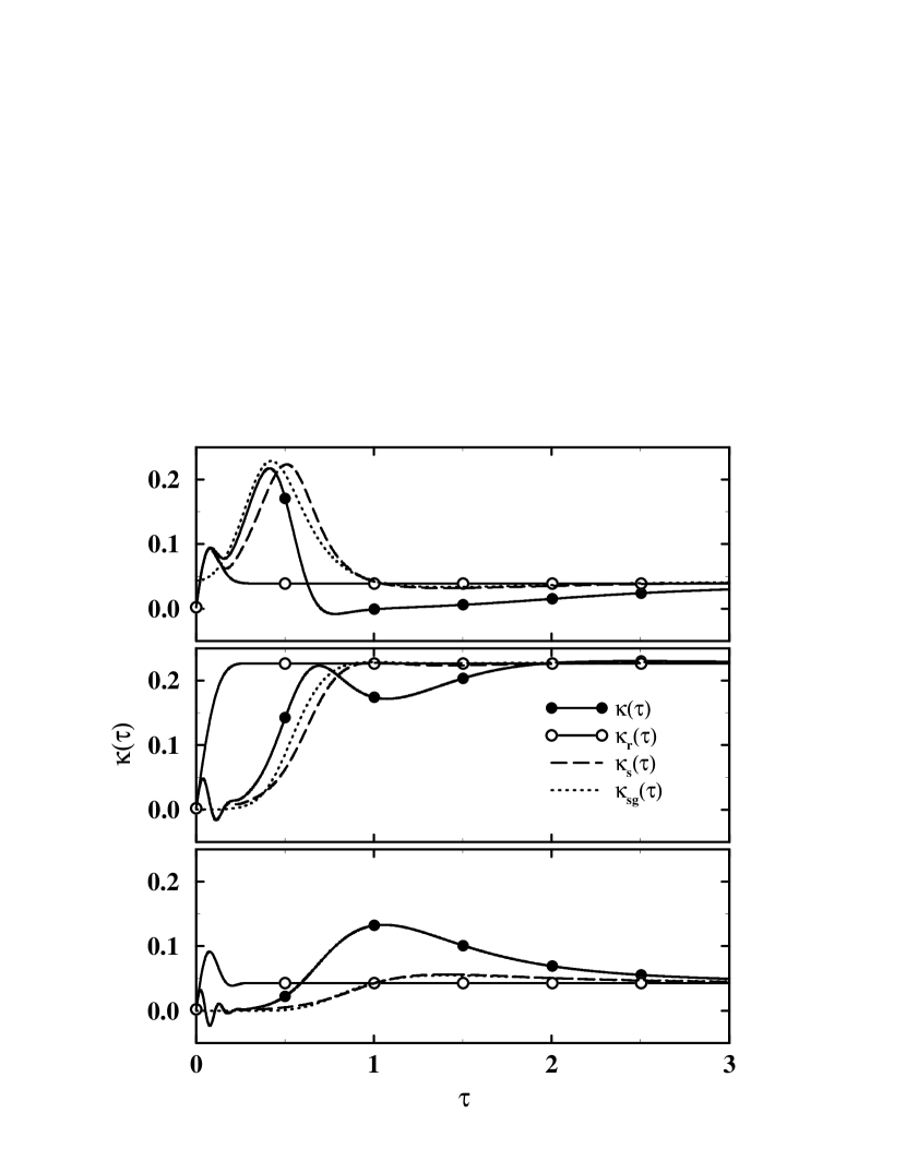
FIG. 1.: Dimensionless nonequilibrium reaction rate $\kappa(\tau)$, Eq. (61), and analogous quantities for $k_{r}(t)$, $k_{s}(t)$, and $k_{sg}(t)$. $\alpha_{{}_{D}}=\alpha_{{}_{A}}=10$ and temperature is zero. The top panel corresponds to $\delta\tilde{\epsilon}=\lambda_{T}-\lambda_{D}$, the middle panel to $\delta\tilde{\epsilon}=\lambda_{T}$, and the bottom panel to $\delta\tilde{\epsilon}=\lambda_{T}+\lambda_{D}$.

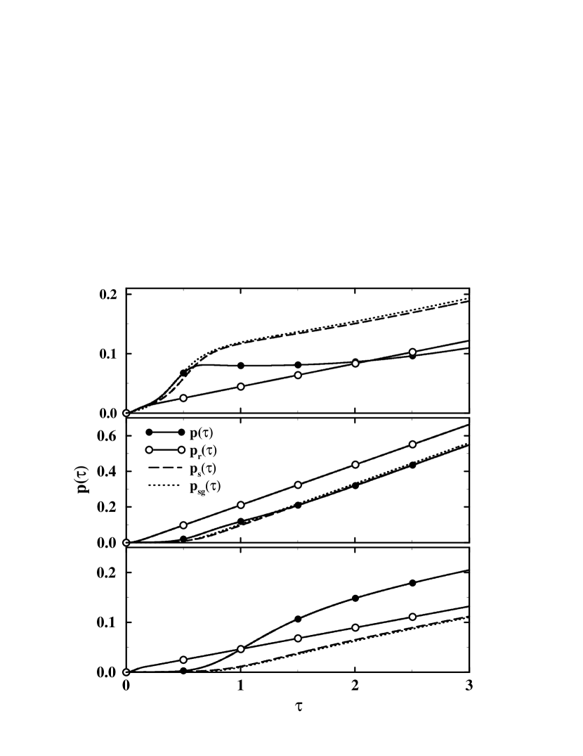
FIG. 2.: Scaled population $p(\tau)$, Eq. (62), and analogous quantities for $k_{r}(t)$, $k_{s}(t)$, and $k_{sg}(t)$. $\alpha_{{}_{D}}=\alpha_{{}_{A}}=10$ and temperature is zero. The top panel corresponds to $\delta\tilde{\epsilon}=\lambda_{T}-\lambda_{D}$, the middle panel to $\delta\tilde{\epsilon}=\lambda_{T}$, and the bottom panel to $\delta\tilde{\epsilon}=\lambda_{T}+\lambda_{D}$.

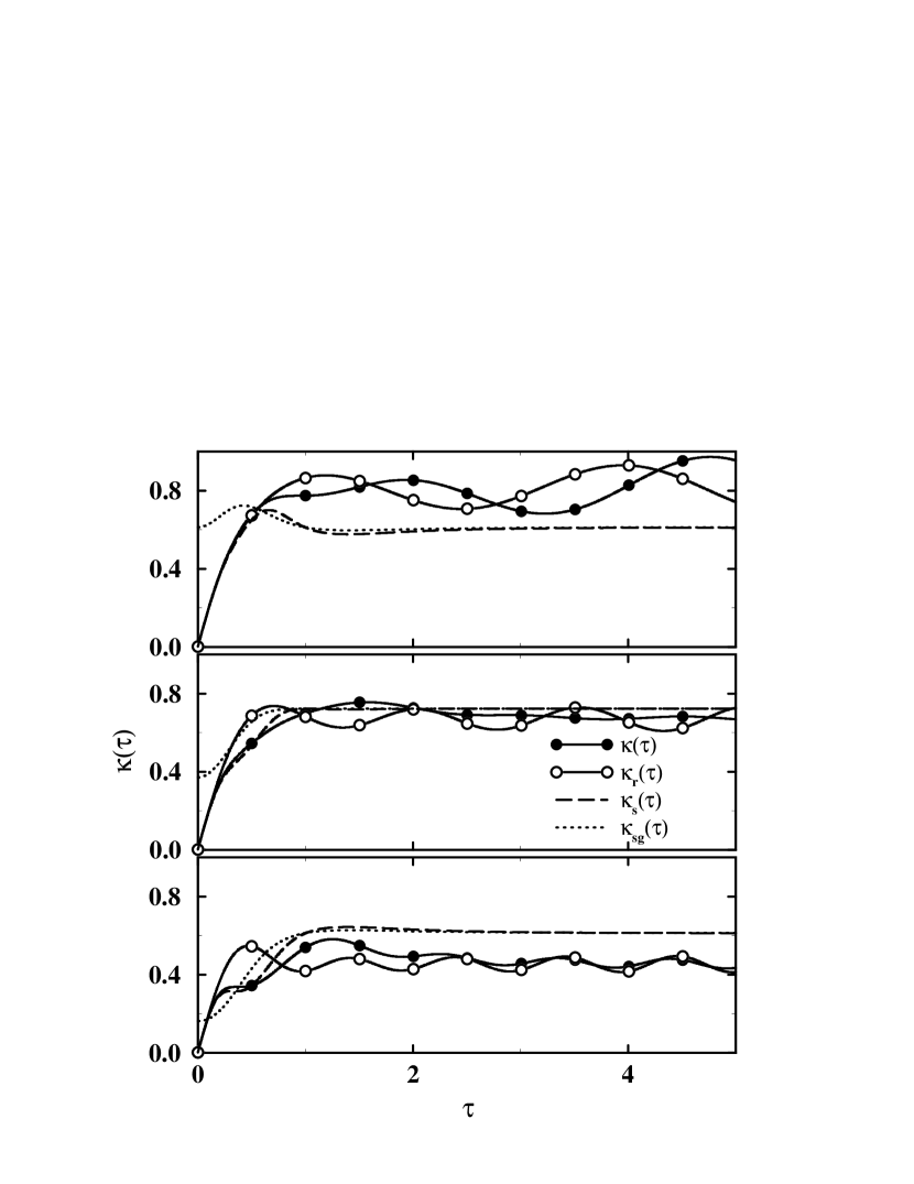
FIG. 3.: Dimensionless nonequilibrium reaction rate $\kappa(\tau)$, Eq. (61), and analogous quantities for $k_{r}(t)$, $k_{s}(t)$, and $k_{sg}(t)$. $\alpha_{{}_{D}}=\alpha_{{}_{A}}=1$ and temperature is zero. The top panel corresponds to $\delta\tilde{\epsilon}=\lambda_{T}-\lambda_{D}$, the middle panel to $\delta\tilde{\epsilon}=\lambda_{T}$, and the bottom panel to $\delta\tilde{\epsilon}=\lambda_{T}+\lambda_{D}$.

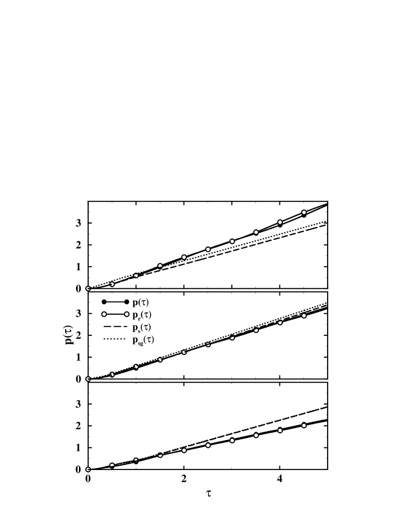
FIG. 4.: Scaled population $p(\tau)$, Eq. (62), and analogous quantities for $k_{r}(t)$, $k_{s}(t)$, and $k_{sg}(t)$. $\alpha_{{}_{D}}=\alpha_{{}_{A}}=1$ and temperature is zero. The top panel corresponds to $\delta\tilde{\epsilon}=\lambda_{T}-\lambda_{D}$, the middle panel to $\delta\tilde{\epsilon}=\lambda_{T}$, and the bottom panel to $\delta\tilde{\epsilon}=\lambda_{T}+\lambda_{D}$.

FIG. 5.: Temperature dependence of $\kappa(\tau)$ (upper panel) and $\kappa_{r}(\tau)$ (lower panel) for $\alpha_{{}_{D}}=\alpha_{{}_{A}}=10$ and $\delta\tilde{\epsilon}=\lambda_{T}-\lambda_{D}$.

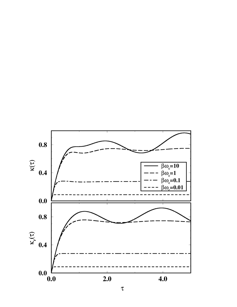
FIG. 6.: Temperature dependence of $\kappa(\tau)$ (upper panel) and $\kappa_{r}$ (lower panel) for $\alpha_{{}_{D}}=\alpha_{{}_{A}}=1$ and $\delta\tilde{\epsilon}=\lambda_{T}-\lambda_{D}$.

REFERENCES

- [1] Th. Förster, Discuss. Faraday Soc. 27, 7 (1953).
- [2] Th. Förster , in Modern Quantum Chemistry, Part III , edited by O. Sinanoglu (Academic Press, New York, 1965).
- [3] D. L. Dexter, J. Chem. Phys. 21, 836 (1953).
- [4] V. M. Agranovich and M. D. Galanin, Electronic excitation energy transfer in condensed matter, North-Holland, Amsterdam, 1982.
- [5] P. Reineker, H. Haken, and H. C. Wolf, Ed., Organic Molecular Aggregates, Springer-Verlag, Berlin, 1983.
- [6] E. J. B. Birks, Excited States of Biological Molecules, John Wiley & Sons, London, 1976.
- [7] D. L. Andrews and A. A. Demidov, Resonance Energy Transfer, John Wiley & Sons, Chichester, 1999.
- [8] G. Cerullo, S. Stagira, M. Zavelani-Rossi, S. De Silvestri, T. Virgili, D. G. Lidzey, and D. D. C. Bradley, Chem. Phys. Lett. 335, 27 (2001).
- [9] S. C. J. Meskers, J. Hübner, M. Oestreich, and H. Bässler, Chem. Phys. Lett. 339, 223 (2001).
- [10] A. R. Buckley, M. D. Rahn, J. Hill, J. Cabanillas-Gonzalez, A. M. Fox, and D. D. C. Bradley, Chem. Phys. Lett. 339, 331 (2001).
- [11] F. V. R. Neuwahl, R. Righini, A. Adronov, P. R. L. Malenfant, and J. M. J. Fréchrt, J. Phys. Chem. B 105, 1307 (2001).
- [12] J. Morgado, F. Cacialli, R. Iqbal, S. C. Moratti, A. B. Holmes, G. Yahioglu, L. R. Milgrom, and R. H. Friend, J. Mater. Chem. 11, 278 (2001).
- [13] X. Hu and K. Schulten, Phys. Today August, 28 (1997).
- [14] V. Sundstrom, T. Pullerits, and R. van Grondelle, J. Phys. Chem. B 103, 2327 (1999).
- [15] T. Renger, V. May, and O. Kühn, Phys. Rep. 343, 137 (2001).
- [16] T. F. Soules and C. B. Duke, Phys. Rev. B 3, 262 (1971).
- [17] S. Rackovsky and R. Silbey, Mol. Phys. 25, 61 (1973).
- [18] B. Jackson and R. Silbey, J. Chem. Phys. 78, 4193 (1983).
- [19] R. Silbey, Annu. Rev. Phys. Chem. 27, 203 (1976).
- [20] M. Grover and R. Silbey, J. Chem. Phys. 54, 4843 (1971).
- [21] R. W. Munn and R. Silbey, J. Chem. Phys. 68, 2439 (1978).
- [22] G. Juzeliunas and D. L. Andrews in Ref. 7.
- [23] C.-P. Hsu, G. R. Fleming, M. Head-Gordon, and T. Head-Gordon, J. Chem. Phys. 114, 3065 (2001).
- [24] H. Sumi, J. Phys. Chem. B 103, 252 (1999).
- [25] K. Mukai, S. Abe, and H. Sumi, J. Phys. Chem. B 103, 6096 (1999).
- [26] K. Mukai, S. Abe, and H. Sumi, J. Lumin. 87-89, 818 (2000).
- [27] G. D. Scholes and G. R. Fleming, J. Phys. Chem. B 104, 1854 (2000).
- [28] G. D. Scholes, X. J. Jordanides, and G. R. Fleming, J. Phys. Chem. B 105, 1640 (2001).
- [29] A. Damjanović, T. Ritz, and K. Schulten, Phys. Rev. E 59, 3293 (1999).
- [30] E. K. L. Yeow and K. P. Ghiggino, J. Phys. Chem. B 104, 5825 (2000).
- [31] S. H. Lin, W. Z. Xiao, and W. Dietz, Phys. Rev. E. 47, 3698 (1993).
- [32] T. Kakitani, A. Kimura, and H. Sumi, J. Phys. Chem. B 103, 3720 (1999).
- [33] A. Kimura, T. Kakitani, and T. Yamato, J. Lumin. 87-89, 815 (2000).
- [34] A. Kimura, T. Kakitani, and T. Yamato, J. Phys. Chem. B 104, 9276 (2000).
- [35] I. Y. Tekhver and V. V. Khizhnyakov, Sov. Phys.-JETP 42, 305 (1976).
- [36] See pages 149-150 of Ref. 4 for a comprehensive list of references.
- [37] H. Sumi, J. Phys. Soc. Japan 51, 1745 (1982).
- [38] H. Sumi, Phys. Rev. Lett. 50, 1709 (1983).
- [39] S. Gnanakaran, G. Haran, R. Kumble, and R. M. Hochstrasser in Ref. 7.
- [40] R. van Grondelle and O. J. G. Somsen in Ref. 7.
- [41] B. A. King, A. de Winter, T. B. McAnaney, and S. G. Boxer, J. Phys. Chem. B 105, 1856 (2001).
- [42] M. Cho and R. J. Silbey, J. Chem. Phys. 103, 595 (1995).
- [43] W. M. Zhang, T. Meier, V. Chernyak, and S. Mukamel, J. Chem. Phys. 108, 7763 (1998).